Spatial Downscaling of Satellite-Based Precipitation and Its Impact on Discharge Simulations in the Magdalena River Basin in Colombia

Introduction

Precipitation is a key component of the water cycle, playing a crucial role in hydro-meteorological and environmental processes (Goovaerts, 2000; Schuurmans and Bierkens, 2006; Langella et al., 2010). An accurate knowledge of precipitation is essential for water resources management and to predict extreme weather events, such as floods and droughts (Arnaud et al., 2002; Vischel and Lebel, 2007; Tramblay et al., 2011).

Precipitation datasets can be obtained from in situ weather stations, but many river basins around the world are still poorly gauged (Loukas and Vasiliades, 2014) or ungauged (Sivapalan et al., 2010). Moreover, measurements from in situ gauges are only representative over a limited distance around the location of the instruments (Collischonn et al., 2008; Bohnenstengel et al., 2011) and their location is often biased toward accessible lower lying areas. These conventional ground observations cannot effectively capture the spatial variability of precipitation and therefore, may be insufficient/non reliable for hydrological modeling (Javanmard et al., 2010).

Satellite-based precipitation datasets may be an attractive alternative to in situ measurements. They cover large areas (many of them have a near-global coverage) over long time periods, reflecting the spatial patterns and temporal variability of precipitation (Adler et al., 2001). A series of gridded global precipitation datasets, including Earth observations, in situ datasets and models, have been developed during the last decades at a regional and global scale (PERSIANN, Hsu et al., 1997; CMORPH, Joyce et al., 2004; GSMaP, Kubota et al., 2007; TRMM, Huffman et al., 2007; ECMWF ERA-Interim, Dee et al., 2011; GPM, Hou et al., 2014; WFDEI, Weedon et al., 2014; CHIRPS, Funk et al., 2015; MSWEP, Beck et al., 2017).

However, recent studies have showed some limitations of satellite-based precipitation datasets in terms of temporal and spatial resolutions when driving a distributed hydrological model to estimate daily discharge values, especially in areas where orographic effects are important (Li et al., 2012; Chen et al., 2013; Khan et al., 2014; Meng et al., 2014). For example, Meng et al. (2014) showed that TRMM precipitation data was not suitable to predict discharge at daily scale in the upstream part of the Yellow River basin, but in contrast it was useful at monthly scale. Moreover, the performance of these satellite-based precipitation datasets might differ depending on basin characteristics, such as size, geographical location, topography, and vegetation cover.

Several authors have developed downscaling, interpolation and aggregation methodologies to increase the spatial resolution of satellite-based precipitation, often in combination with ground observations (see overview in Table 1). The resulting precipitation datasets may provide a better representation of the spatial variability of precipitation to be used for hydrological applications.

TABLE 1

Table 1. Summary of relevant studies where downscaling methodologies are developed to increase the spatial resolution of satellite-based precipitation datasets.

There exist a large number of Earth observations data available on hydro-meteorological variables that are related to precipitation, including Normalized Difference Vegetation Index (NDVI), Enhanced Vegetation Index (EVI), Leaf Area Index (LAI), temperature, and elevation. The auxiliary information derived from these variables can be combined with satellite-based precipitation datasets to increase their spatial resolution. So far most studies focused on the use of NDVI as proxy to downscale precipitation (Immerzeel et al., 2009; Chen et al., 2014; Hunink et al., 2014). Moreover, only one study used different satellite-based precipitation datasets to TRMM product (Ceccherini et al., 2015). Also, most studies used regression analyses with model parameters spatially constant (multiple linear, polynomial, exponential, etc.), assuming a spatial stationarity of the relationship between precipitation and the proxy variables (Duan and Bastiaanssen, 2013; Fang et al., 2013; Park, 2013; Hunink et al., 2014). In addition, most studies limited their analyses to satellite-based precipitation datasets and did not take full advantage of all available data sources, combining remotely sensed and in situ observations (Ceccherini et al., 2015; Xu et al., 2015; Ezzine et al., 2017). In this study, a new downscaling methodology based on earlier work of Duan and Bastiaanssen (2013), Hunink et al. (2014) and Ceccherini et al. (2015) was developed using four proxies (EVI, elevation, slope, and aspect) in a Geographically Weighted Regression (GWR) algorithm, in which regression parameters varied with location. Four different satellite-based precipitation datasets, including CMORPH, MSWEP, PERSIANN, and TRMM, were downscaled with this new methodology from 25 to 1 km resolution and combined with in situ observations from March 2000 to December 2012 in the Magdalena River basin in Colombia.

Furthermore, previous studies did not analyze the impact of precipitation downscaling on discharge simulations. Several authors demonstrated that spatial distribution of precipitation is one of the main sources of uncertainty in hydrological modeling (Berne et al., 2004; Sangati and Borga, 2009). The impact of spatial representation of precipitation on hydrological model estimates is complex and it depends on the type of precipitation (Bell and Moore, 2000), the hydrological characteristics of the basin (soils, geology, river morphology, vegetation cover, etc.), the hydrological model structure (Koren et al., 1999) and the considered spatial and time scales (Segond et al., 2007). Some studies stated that the impact of precipitation spatial resolution on discharge simulation was not significant (Gascon et al., 2015; Nkiaka et al., 2017). However, most studies (Andréassian et al., 2001; Smith et al., 2004; Schuurmans and Bierkens, 2006; Wagener et al., 2007; Arnaud et al., 2011; Fu et al., 2011; Zoccatelli et al., 2011; Emmanuel et al., 2012; Zhao et al., 2013; Lobligeois et al., 2014) showed that better model performances were obtained when representation of the spatial variability of precipitation was improved. In this study, the impact of precipitation spatial resolution on discharge simulations was investigated. Non-downscaled and downscaled precipitation datasets were used to force the distributed hydrological model OpenStreams wflow-hbv. Lastly, the effect on discharge of a decrease in the number of rain gauge stations used for precipitation downscaling was analyzed. More than 40 hydrological simulations were carried out with different network densities of in situ precipitation data (Vischel and Lebel, 2007; Bardossy and Das, 2008).

This study aims to analyze how sensitive discharge simulations are to precipitation spatial resolution using Earth observations and ground measurements. Developing a new downscaling methodology which integrates satellite-based and in situ data and understanding its impact on discharge estimates may have broader implications for similar but data-poor river basins globally.

Study Area

The study area is the Magdalena River basin (Figure 1), which is the largest fluvial system in Colombia, draining an area of ~257,000 km² (about 24% of the total territory of the country). The Magdalena River originates from headwaters in the Colombian Andes at an elevation of 3,700 m and it runs for 1,612 km into the Western Caribbean, in the Atlantic Ocean (Restrepo and Kjerfve, 2000). The main tributary of the Magdalena River is the Cauca River on the Western part of the watershed.

FIGURE 1

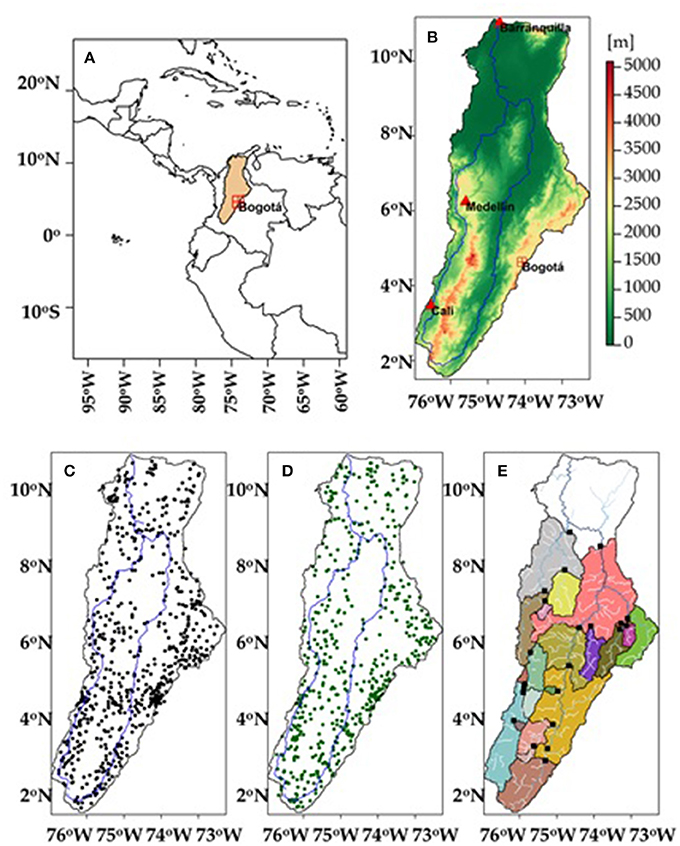
Figure 1. (A) Location of the Magdalena River basin in Colombia; (B) topography, main river network and urban areas within the basin; (C) weather stations used for deriving the downscaled precipitation datasets; (D) weather stations used for evaluation, and (E) discharge stations and drainage sub-basins.

Average annual precipitation for the Magdalena River basin is ~2,150 mm year⁻¹, with large inter-annual variability, especially due to the effect of the El Niño-Southern Oscillation (ENSO) phenomenon (Hoyos et al., 2013). Precipitation ranges from 1,000 mm year⁻¹ in the eastern mountains to more than 5,000 mm year⁻¹ in the western region of the basin. The area under snow influence represents less than 0.1% of the total area of the watershed. The climate in the basin is characterized by two wet periods (March-May and October-November) and two dry periods (December-March and June-September). Average annual air temperature is ca. 28°C and average annual evapotranspiration is ~1,630 mm year⁻¹. Average annual discharge at the outlet of the basin is ~7,200 m³ s⁻¹, varying from 4,050 m³ s⁻¹ in March to 10,200 m³ s⁻¹ in November (Camacho et al., 2008).

The main cities of Colombia, including Cali, Bogotá, Medellín, and Barranquilla are situated in the Magdalena River basin and almost 80% of Colombia's population lives within the basin. During the last decades, the basin has witnessed considerable changes in land use, water, soil losses and a rapid increase of natural resources exploitation due to the economic development in the area (Restrepo and Syvitski, 2006). This recent situation has increased the pressure on the Magdalena River basin, which is the main source for human water consumption, agriculture, hydropower generation, industrial activities and ecosystems support.

Some recent initiatives have been carried out in the basin in order to improve water resources management for the diverse demands and at different scales, increasing availability, and quality of hydro-meteorological data and models (Angarita et al., 2013; Boodoo et al., 2014; Restrepo et al., 2015; Cruz-Roa et al., 2017). The region frequently suffers from extreme events, such as the large flooding event caused by the 2010–2011 La Niña phenomenon (Hoyos et al., 2013) and the severe droughts as a result of the 2015–2016 El Niño phenomenon (Hoyos et al., 2017). Besides, a complex terrain orography, make challenging to accurately estimate water resources in the basin, including precipitation and discharge.

Data

Precipitation Data

Satellite-Based Precipitation Data

Four satellite-based precipitation datasets were used in this study:

- Climate Prediction Center MORPHing technique-CMORPH:

CMORPH precipitation dataset is derived from passive microwave observations from low-Earth orbiting satellites exclusively (such as AMSR-E and TMI aboard NASA's Aqua and TRMM spacecraft), and whose features are transported via spatial propagation information entirely obtained from geostationary satellite infrared data. The technique applied to derive CMORPH precipitation data is not a precipitation estimation algorithm, but a means to combine precipitation estimates from existing microwave precipitation algorithms. Infrared data are used to transport the microwave-derived precipitation features during periods when microwave data are not available at a location (Joyce et al., 2004).

- Multi-Source Weighted-Ensemble Precipitation-MSWEP:

MSWEP v1.0 precipitation dataset combines a wide range of data sources, including gauges, satellites and atmospheric reanalysis models. The long-term mean of MSWEP is based on the elevation-corrected CHPclim dataset but replaced with more accurate regional datasets where available. A correction for gauge under-catch and orographic effects is introduced by inferring catchment-average P from discharge observations at 13,762 stations across the globe. The temporal variability of MSWEP precipitation was determined by weighted averaging precipitation anomalies from seven precipitation datasets: two based solely on interpolation of in situ observations (CPC Unified and GPCC), three on satellite remote sensing (CMORPH, GSMaP-MVK and TMPA 3B42RT) and two on atmospheric model reanalysis (ERA-Interim and JRA-55). For each grid cell, the weight assigned to the gauge-based estimates was calculated from the gauge network density, while the weights assigned to the satellite- and reanalysis- based estimates were calculated from their comparative performance at the surrounding gauges (Beck et al., 2017).

- Precipitation Estimation from Remotely Sensed Information using Artificial Neural Networks-PERSIANN:

PERSIANN precipitation dataset is derived using artificial neural network function classification/approximation procedures based on both infrared and daytime visible imagery by geostationary satellites (such as GOES-8 and GMS-5). Model parameters of PERSIANN precipitation algorithm are updated from passive microwave observations from low-Earth orbiting satellites (Hsu et al., 1997).

- Tropical Rainfall Measuring Mission—Multi-satellite Precipitation Analysis 3B42—TRMM:

TRMM precipitation dataset combines remote observations such as precipitation radar, passive microwave and infrared from multiple low-Earth orbiting and geostationary satellites and ground observations. Version 7 TRMM precipitation estimated by the 3B42 algorithm was used in this study. TRMM precipitation estimates are produced in four stages: (i) the passive microwave precipitation estimates are calibrated and combined, (ii) the infrared precipitation estimates are created using the calibrated microwave precipitation, (iii) the microwave and infrared estimates are combined, and (iv) rescaling to monthly data is applied (Huffman et al., 2007).

Satellite-based precipitation data were provided at 25 km spatial resolution by the Consiglio Nazionale delle Richerche (CNR) in Italy, as part of the FP7 European project eartH2Observe (Levizanni and Dorigo, 2017). A non-exhaustive overview of the satellite-based precipitation datasets is included in Table 2.

TABLE 2

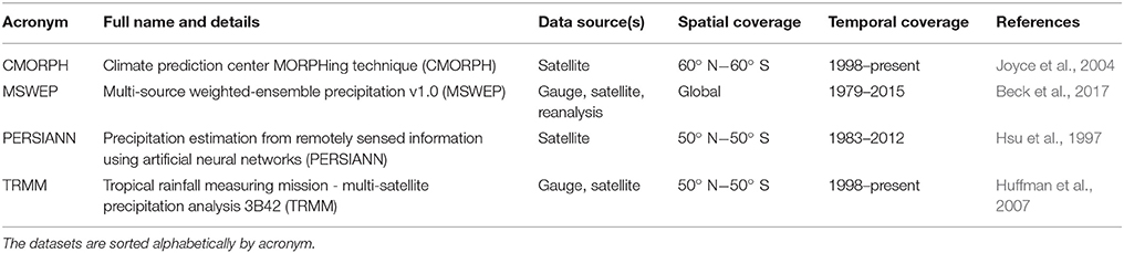
Table 2. Satellite-derived precipitation data.

In Situ Precipitation Data

Precipitation data from 1,118 weather stations within the Magdalena River basin were used. Daily precipitation data was provided by the Institute of Hydrology, Meteorology, and Environmental Studies (IDEAM) of Colombia, covering the period from March 2000 to December 2012. The locations of the weather stations are shown in Figure 1.

Air Temperature and Evapotranspiration Data

Daily air temperature and evapotranspiration data were obtained from the WATCH Forcing Data methodology applied to ERA-Interim reanalysis data (WFDEI) at a spatial resolution of ca. 50 km (Weedon et al., 2014). The FAO Penman-Monteith equation was used to derive reference potential evapotranspiration. Air temperature and reference potential evapotranspiration were downscaled from 50 to 1 km resolution using the e2o-downscaling-tools (Weiland et al., 2015; Schellekens and Weiland, 2017).

Vegetation Response Data: Enhanced Vegetation Index

The Enhanced Vegetation Index (EVI) is an indicator of plant greenness or photosynthetic activity based on how different surfaces reflect different wavelengths of light. The EVI was developed as an alternative vegetation index to overcome some limitations of the Normalized Difference Vegetation Index (NDVI), such as saturation of the signal in densely vegetated and humid areas. The EVI was developed to maintain high sensitivity to changes in areas with dense biomass, to reduce the influence of the atmospheric conditions in the index value and to minimize canopy background variations. Some previous studies proved successful EVI applications in areas having high biomass, including the Amazon forest (Huete et al., 2002; Bradley et al., 2011). In this study, EVI data (MOD13A2) derived from the Moderate Resolution Imaging Spectroradiometer (MODIS) on board the Terra satellite (from hereafter referred as EVI) were used. EVI data are provided every 16 days at 1 km spatial resolution. The post-processing steps include a re-projection and masking of water bodies. Water bodies may present negative EVI values leading to problems in the subsequent regression. Therefore, water bodies were masked and corresponding EVI values were removed. Subsequently, EVI values were interpolated for those areas. The water body mask was obtained from the NASA Shuttle Radar Topography Mission (SRTM) Water Body Data dataset developed by the National Geospatial-Intelligence Agency (SWBD, 2017).

Elevation, Slope, and Aspect Data

Digital Elevation Model (DEM) data from the NASA Shuttle Radar Topographic Mission (SRTM) distributed by the United States Geological Survey (USGS) was used. The vertical error of the DEM is less than 16 m (Sun et al., 2003). The DEM at a spatial resolution of 3 arc-second (~90 m) was resampled (averaged) to 1 km resolution. Slope and aspect were extracted from the DEM using QGIS (QGIS, 2017).

Discharge Data

Daily discharge data from 22 gauging stations along the Magdalena River and its tributaries were used for hydrological model evaluation and provided by the Institute of Hydrology, Meteorology and Environmental Studies (IDEAM) of Colombia. Figure 1 shows the location of discharge stations and Table 3 includes the location, river and sub-basin area for each discharge station.

TABLE 3

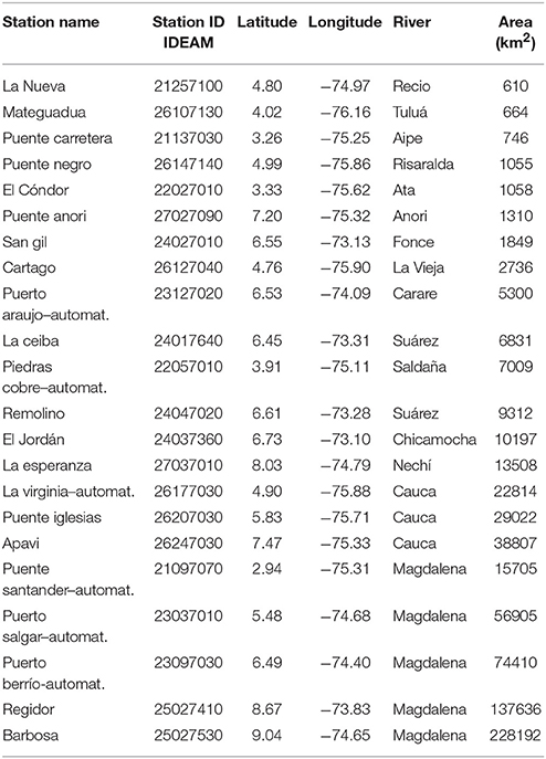
Table 3. Discharge stations used for validation.

Methodology

Firstly, the four satellite-based precipitation datasets were downscaled to a finer spatial resolution of 1 km. Secondly, an independent evaluation of precipitation was carried out using in situ precipitation data before and after downscaling. Thirdly, satellite-based and in situ precipitation datasets at different spatial resolutions were used to force the distributed hydrological model OpenStreams wflow-hbv and the impact of precipitation spatial resolution on modeled discharge was evaluated.

Downscaling Precipitation

A new precipitation downscaling model based on earlier work of Duan and Bastiaanssen (2013), Hunink et al. (2014), and Ceccherini et al. (2015) was developed and applied to estimate precipitation at 1 km resolution from the four satellite-based precipitation datasets. Model parameters and variables are listed in Table 4. The downscaling procedure consists of three main steps:

1. Spatial downscaling of monthly precipitation

2. Merging monthly downscaled precipitation with in situ observations

3. Disaggregating from monthly precipitation into daily values

TABLE 4

Table 4. List of variables and parameters used in the precipitation downscaling model.

Spatial Downscaling of Monthly Precipitation

An exhaustive review of relevant studies where spatial downscaling methodologies were developed to increase the spatial resolution of satellite-based precipitation datasets was done. These downscaling methodologies use auxiliary information from environmental variables available at fine spatial resolutions, such as vegetation response, topographical characteristics (elevation, slope, aspect, etc.), and humidity, as predictors to estimate precipitation. In this study, four environmental variables were used as a proxy to downscale precipitation, including the vegetation response (EVI), elevation, slope, and aspect. These variables were selected based on the hydro-meteorological characteristics of the Magdalena River basin, considering the main factors that influence precipitation in the region.

Initially, the relation between EVI and precipitation was analyzed. The sensitivity of the vegetation state to precipitation is cumulative (Immerzeel et al., 2005; Gessner et al., 2013), which means that vegetation indexes, such as NDVI and EVI, respond to precipitation with a lag time. Quiroz et al. (2011) estimated the lag time in 1–3 months and Hunink et al. (2014) considered a lag time of 1 week in their weekly regression models between precipitation, elevation, climatology and NDVI. In this study, EVI was used to avoid limitations of NDVI [see section Vegetation response data: Enhanced Vegetation Index (EVI)]. An analysis was carried out to estimate the lag time between precipitation and EVI. Basin average values of precipitation and EVI were calculated for the entire time period (March 2000–December 2012). Correlation values between precipitation and EVI were obtained considering lag times between 1 week and 3 months (Table S1). The highest correlation values were obtained with a lag time between precipitation and EVI of 1 month.

Similarly, the relation between topography (elevation, slope and aspect) and precipitation was analyzed. Correlation values between elevation and precipitation were obtained at daily, weekly, and monthly temporal scales. The highest correlation values were obtained at monthly scale and hence, precipitation was estimated based on vegetation response and topography at monthly scale.

Between the various functions that could be used to relate precipitation with vegetation response and topography (linear, second order polynomial, power, exponential, etc.), a geographically weighted regression (GWR) model was selected, which is a local form of multiple linear regression. The GWR model is able to capture the spatial variability in the relationship between precipitation, vegetation response and topography, which would not be noticed in the other regression methods. Moreover, Ceccherini et al. (2015) successfully downscaled precipitation using the GWR method in South America, where the Magdalena River basin is located.

The specific steps used for spatial downscaling of monthly precipitation are described as follows:

(i) DEM, SLOPE, ASPECT, and monthly EVI were aggregated by pixel averaging from the spatial resolution of 1 km to the spatial resolution of the satellite-based precipitation datasets, 25 km.

(ii) Using the GWR model, monthly precipitation, P, was estimated based on DEM, SLOPE, ASPECT and monthly EVI at 25 km resolution. The GWR supplied the coefficient of determination of the regression r² per pixel. All possible linear combinations of variables (separately) were analyzed because in some cases the relationship between precipitation and auxiliary variables was stronger excluding some of them. For example, the relationship between precipitation and EVI may be weak in areas where the land use was fragmented, hence excluding EVI improved the model regression performance. The following GWR models resulted in higher r²:

$\begin{array}{l}{P}_j=a_j+b_j·DEM+c_j·SLOPE+d_j·ASPECT\\ +e_j·EV{I}_{j+1}& (1)\end{array}$

$\begin{array}{rc}{P}_j=a_j+b_j·DEM& (2)\end{array}$

$\begin{array}{rc}{P}_j=a_j+b_j·DEM+c_j·SLOPE+d_j·ASPECT& (3)\end{array}$

$\begin{array}{rc}{P}_j=a_j+b_j·DEM+e_j·EV{I}_{j+1}& (4)\end{array}$

where a_j, b_j, c_j, d_j, and e_j were the GWR model parameters at month j, varying with location and P_j is the estimated precipitation at 25 km resolution at month j. For each grid cell, the P_j and the GWR model parameters associated with the highest coefficient of determination r² were selected and used for further downscaling.

(iii) Residuals were computed as the difference between P_j and the initial precipitation dataset at 25 km resolution. Assumptions of normality, non-autocorrelation and homocedasticity of the residuals were checked. The GWR models that produced residuals which did not meet these assumptions were rejected. Normality of the residuals was verified using histograms of the residuals and the Shapiro-Wilk test (Shapiro and Wilk, 1965). Homocedasticity was checked with the Breusch-Pagan test (Breusch and Pagan, 1979) and autocorrelation was verified with the Durbin-Watson test (Durbin and Watson, 1951).

(iv) The GWR model parameters were downscaled to 1 km resolution using a cubic spline tension interpolator (Ceccherini et al., 2015).

(v) Monthly downscaled precipitation at 1 km resolution, PD_j, was estimated based on the obtained GWR model parameters and DEM, SLOPE, ASPECT, and monthly EVI at 1 km resolution as follows:

$\begin{array}{l}P{D}_j=a_j+b_j·DEM+c_j·SLOPE+d_j·ASPECT\\ +e_j·EV{I}_{j+1}& (5)\end{array}$

Merging Monthly Downscaled Precipitation With in Situ Observations

To take full advantage of precipitation datasets available in the region, downscaled satellite-derived precipitation can be merged with in situ measurements from rain gauge stations. Some previous downscaling studies (Immerzeel et al., 2009; Duan et al., 2012; Duan and Bastiaanssen, 2013) compared different methods to optimally combine in situ and satellite-based precipitation datasets. In this study, the specific steps used for merging monthly downscaled precipitation with in situ observations are described as follows:

(vi) Monthly downscaled precipitation values at 1 km resolution were extracted for the location of weather stations and the difference between in situ precipitation and monthly downscaled precipitation for each station was calculated. These differences or residuals were spatially interpolated using a cubic spline tension interpolator to a resolution of 1 km, obtaining Δ_j. Inverse distance weighting (IDW), nearest neighbor algorithm and cubic spline interpolation methods were tested and cubic spline outperformed the other methods.

(vii) By adding PD_j to the residuals Δ_j, monthly downscaled precipitation are combined with in situ measurements at 1 km resolution, obtaining PDI_j:

$\begin{array}{rc}PD{I}_j=P{D}_j+{\Delta }_j& (6)\end{array}$

Disaggregating From Monthly Precipitation Into Daily Values

For hydrological modeling and prediction of daily discharge, daily precipitation estimates are needed. However, the procedure described until here estimated precipitation at monthly temporal scale. In this step, the fraction of precipitation per day derived from precipitation datasets at 25 km resolution was used to disaggregate monthly downscaled precipitation at 1 km resolution into maps at daily time scale. Duan and Bastiaanssen (2013) applied a similar methodology to disaggregate annual to monthly precipitation. The specific steps for disaggregating from monthly downscaled precipitation into daily values are described as follows:

(viii) Precipitation at 25 km resolution that occurs during the ith day was divided between the monthly total precipitation to obtain the fraction of precipitation per day i:

$\begin{array}{rc}{F}_i=\frac{P_i}{{\displaystyle {\sum }_{i=1}^n}{P}_i}& (7)\end{array}$

where n was the number of days of each month.

(ix) The fractions of precipitation per day at 25 km resolution, F_i, were interpolated using a cubic spline tension interpolator into a spatial resolution of 1 km, obtaining FD_i.

(x) Monthly downscaled precipitation at 1 km resolution was multiplied with the corresponding fractions to obtain daily precipitation:

$\begin{array}{rc}PD{I}_i=F{D}_i·PD{I}_j& (8)\end{array}$

Precipitation Evaluation

To ensure an independent evaluation of precipitation before and after downscaling, a split sample approach of the 1,118 weather stations was used. The precipitation of 616 stations was used for deriving the downscaled precipitation datasets and the remaining 502 stations were used for evaluation. These two station groups were randomly selected such that they were equally distributed in space over the catchment.

The accuracy of the different precipitation datasets at 25 and 1 km resolution was assessed by a number of commonly used performance indicators (Immerzeel et al., 2009; Ceccherini et al., 2015): coefficient of determination (r²), difference between satellite-based, and in situ precipitation values and Root Mean Square Error (RMSE).

Hydrological Modeling and Discharge Evaluation

Hydrological Modeling

The distributed hydrological model OpenStreams wflow-hbv (Schellekens, 2014) was used. The OpenStreams wflow-hbv model is based on the HBV-96 model (Sælthun, 1996) and it is programmed in the PCRaster-Python environment (Karssenberg et al., 2010). It is freely available through the OpenStreams project (Schellekens, 2016).

OpenStreams wflow-hbv is applied on a cell-by-cell basis and for each grid cell it determines the water balance considering the following three components: precipitation-snow routine (including interception), soil moisture routine and runoff response routine. To simulate the different runoff processes, the soil is divided into two layers: the upper and lower zone. Daily total runoff of every grid cell results from adding direct runoff, interflow from the upper soil zone and baseflow from the lower soil zone. The total runoff is accumulated from all grid cells and routed using a kinematic wave function to obtain river discharge. A schematic representation of the hydrological model is given in Figure 2.

FIGURE 2

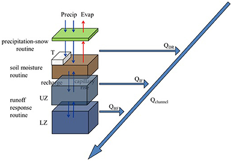
Figure 2. OpenStreams wflow-hbv model structure.

Land cover information was obtained from the global land cover map GlobCover-2009 derived from observations of MERIS sensor on board the ENVISAT satellite mission (Arino et al., 2010). Soil information was obtained from the Food and Agriculture Organization (FAO) Digital Soil Map of the World (DSMW, 2007). The model version used in this study does not include reservoirs. Daily simulations at 1 km resolution were carried out for the time period March 2000 to December 2012.

Discharge Evaluation

The daily precipitation datasets at 25 and 1 km resolutions were used to force the OpenStreams wflow-hbv model. Firstly, in situ daily precipitation values at weather locations were interpolated using the inverse distance weighting algorithm to create spatial maps at 1 km resolution (various interpolation techniques were tested, including splines, inverse distance weighting and kriging with external drift, and inverse distance weighting outperformed the other methods). Then, OpenStreams wflow-hbv was calibrated and validated using interpolated in situ precipitation during 2000–2012. The year 2000 was used to spin up the model until reaching a dynamical steady state. The time periods 2001–2004 and 2005–2012 were used for calibration and validation, respectively. Kling-Gupta efficiency (KGE; Gupta et al., 2009) was selected as the optimization criterion, to avoid problems that could occur when Nash-Sutcliffe efficiency (NSE; Nash and Sutcliffe, 1970) is used for model calibration (e.g., high sensitivity to extreme values). Model parameters were calibrated to optimize KGE values at 22 discharge stations.

Secondly, the impact on discharge simulations of a decrease in the number of weather stations used in the downscaling procedure was analyzed. Fourteen weather station networks composed of 0, 4, 8, 10, 20, 30, 40, 50, 60, 80, 100, 200, 400, and 616 stations were selected from the 616 rain gauges used for deriving the downscaled precipitation datasets. A stratified sampling technique was used to build the weather station networks. This technique avoids problematic networks that may result from simple randomly sampling, aiming uniform station networks homogenously distributed over the basin. The specific steps to build each station network are described as follows:

(i) The area of the basin was divided into different grid cells using a spatial resolution of ca. 50 km.

(ii) A random sample of size n_i from each grid cell was extracted aiming for n₁ + n₂ +…+ n_k = n, where n is the total number of weather stations of the network (4, 8, 10, 20, 30, 40, 50, 60, 80, 100, 200, 400). Minimum distance between stations was considered to avoid taking stations that were very close to each other.

(iii) Step (ii) was repeated 10 times to generate multiple realizations of each subset of stations per grid cell of size n_i, which results in 10 different configurations of the entire station network. This reduces the effect of poorly distributed networks and the influence of undetected inhomogeneous station records.

(iv) Precipitation values at weather stations were interpolated using the inverse distance weighting algorithm to create spatial maps at 1 km resolution for each of the 10 station network configurations.

(v) Precipitation derived from each of the 10 station network configurations was evaluated by calculating r² and RMSE and the spatial configuration with the highest performance was selected.

This technique was applied repeatedly to obtain networks of n number of rain gauge stations. Similar sampling approaches have been successfully used in previous studies to analyze the effect of sample size on precipitation and hydrological modeling (Janis et al., 2004; Bardossy and Das, 2008; Xu et al., 2013).

Every generated precipitation dataset was used to force the OpenStreams wflow-hbv and the effect on simulated discharge was evaluated. Various statistical indicators were used to evaluate model performance: KGE, Pearson's correlation coefficient (r) and RMSE. KGE equally measures bias and differences in timing and amplitude, whereas r measures mainly differences in timing of high and low discharge and RMSE differences in magnitude.

Results

Precipitation Evaluation

Assessing the Performance of Precipitation Datasets at 25 km

In order to evaluate how well satellite-based precipitation datasets at 25 km resolution perform, Figures 3a–c show the boxplots of three performance indicators, including the difference (Figure 3a), RMSE (Figure 3b), and r² (Figure 3c) between monthly satellite-based and in situ observed precipitation. From Figure 3a, MSWEP and TRMM precipitations show the largest agreement with in situ data (differences close to 0). CMORPH slightly underestimates precipitation, while PERSIANN largely overestimates it. From Figure 3b, PERSIANN exhibits the largest RMSE values, followed by CMORPH. Low values of RMSE come from MSWEP and TRMM. From Figure 3c, MSWEP provides the highest r² values. High r² values are also displayed with TRMM, while CMORPH and PERSIANN show lower values. To complete the evaluation of satellite-based precipitation datasets at 25 km resolution, Figure 3d shows the boxplot of climatology of monthly satellite-based and in situ observed precipitation. MSWEP and TRMM capture the intra-annual variability of precipitation during the year well, whereas CMORPH and PERSIANN show larger differences with ground data. PERSIANN displays a good agreement during the dry period from December to March, but highly overestimates precipitation during the rest of the year, especially from May to September. CMORPH is able to reproduce precipitation variability, but with a consistent underestimation. Precipitation differences could be due to the fact that MSWEP and TRMM precipitation data sources include in situ observations, whereas CMORPH and PERSIANN do not.

FIGURE 3

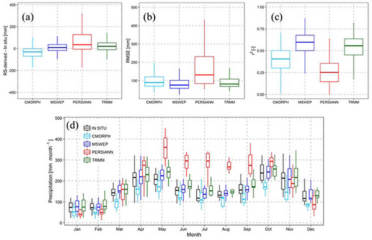
Figure 3. Boxplots of (a) the difference, (b) RMSE, and (c) r² between monthly satellite-based precipitation at 25 km resolution and observed precipitation for the 502 validation weather stations. (d) Boxplot of climatology of monthly satellite-based and observed precipitation at 25 km resolution (average of 502 validation weather stations).

Precipitation Downscaling Analysis

Figure 4 summarizes the results derived from the GWR analysis at 25 km resolution. GWR model parameters and model variables to estimate MSWEP precipitation are shown for May 2003. Although in the GWR model, slope and aspect were considered as predictors, results indicated that their contribution is minimal. Therefore and for practical reasons, Figure 4 shows only EVI and DEM predictors and the associated model parameters. Model parameters show different spatial patterns. Slope parameter for DEM is positively related to precipitation in the northern and southern parts of the basin, but a negative relationship exists in the central region (high precipitation and low elevation). Slope parameter for EVI shows positive values for the relationship between EVI and precipitation in most part of the basin, with higher values in the central-eastern region.

FIGURE 4

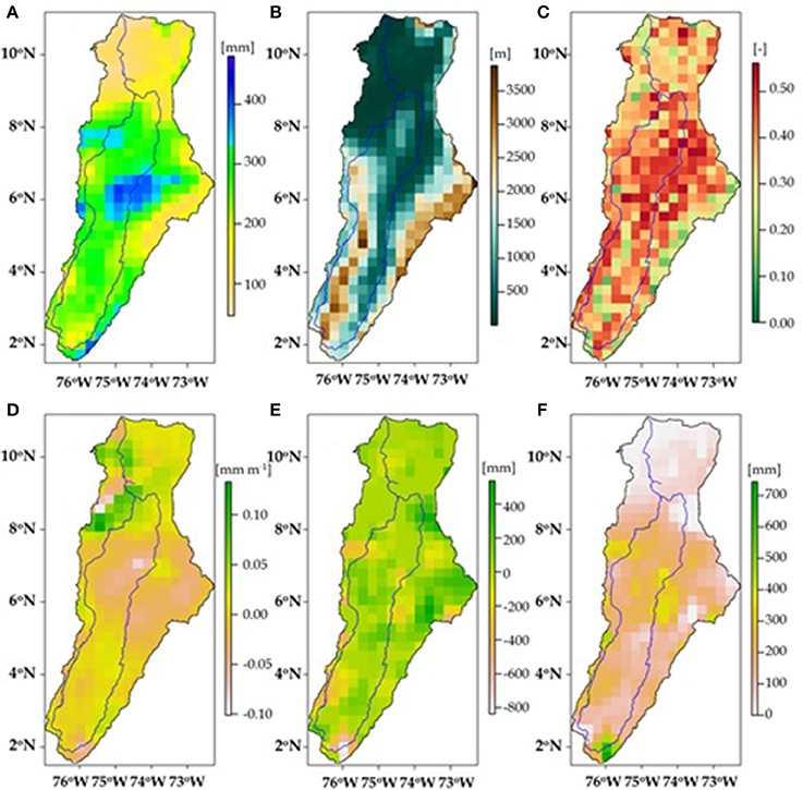
Figure 4. Spatial distribution of (A) average monthly MSWEP precipitation, (B) DEM, (C) average monthly EVI, (D) GWR slope parameter for DEM, (E) GWR slope parameter for EVI, and (F) GWR intercept in May 2003 at 25 km resolution.

Once the GWR analysis was completed, downscaled satellite-based datasets were merged with in situ observations to estimate precipitation at 1 km resolution. Figure 5 shows precipitation datasets at 25 km resolution (first row), at 1 km resolution (second row), and the residuals at 1 km resolution (third row) for April 2000. Figure 5 reveals that precipitation in the central part of the basin is indeed much higher (~400 mm month⁻¹) than in northern and southern regions (~100 mm month⁻¹). The range of values is consistent with the monthly precipitation analysis done by IDEAM in Colombia (IDEAM, 2017). Spatial patterns of CMORPH, MSWEP, and TRMM precipitation datasets are similar, except for some areas in the south-eastern part of the basin (CMORPH in the first row of Figure 5). PERSIANN differs in the spatial variability of precipitation, providing higher estimates in most of the basin than the remaining precipitation datasets.

FIGURE 5

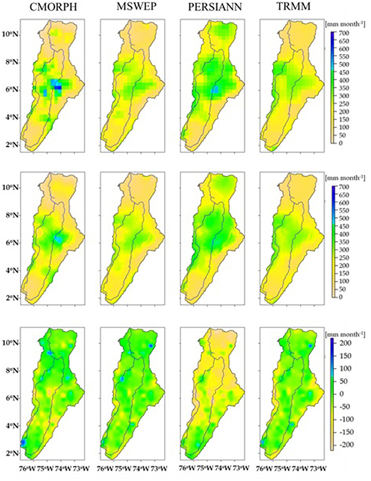
Figure 5. Spatial distribution of CMORPH, MSWEP, PERSIANN, and TRMM precipitation datasets at 25 km (P, first row) and 1 km (PD, second row) and spatial distribution of residuals at 1 km (Δ, third row) for April 2000.

The general precipitation patterns are well captured by the PD (second row), with the central part wetter, corresponding well with the original precipitation datasets. Residuals (Δ, third row) show the amount of precipitation that cannot be explained by the GWR model compared to in situ measurements. Negative residuals (yellow) indicate regions where precipitation is overestimated. Positive residuals (blue) depict areas where precipitation is less than expected according to in situ information. Residuals of CMORPH, MSWEP, and TRMM are close to zero (green) in the majority of the basin, whereas residuals of PERSIANN are around −150 mm month⁻¹ with values closer to zero in the southern part. In all precipitation datasets, some isolated small areas with higher residuals can be observed, which could be related to the complex orography and the strong spatial variability of precipitation.

Assessing the Performance of Downscaled Precipitation Datasets

To assess the performance of downscaled precipitation datasets r², the difference between satellite-based and in situ precipitations and RMSE were calculated. Each indicator was obtained for each weather station and was plotted and spatially interpolated using cubic splines. Figure 6 shows the difference between precipitation datasets at 25 km resolution (P, first row) and at 1 km resolution (PDI, second row) and in situ observations, giving an indication of the accuracy of the original and final precipitation datasets over the entire basin.

FIGURE 6

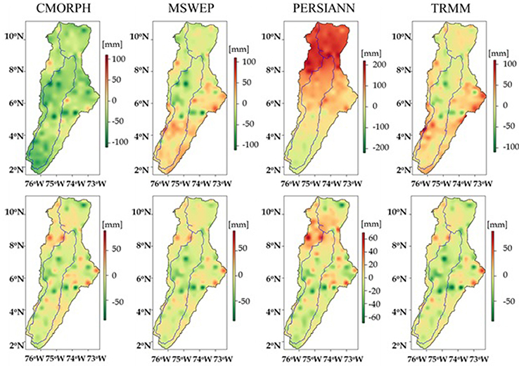
Figure 6. Interpolated difference between CMORPH, MSWEP, PERSIANN, and TRMM precipitation datasets at 25 km (P, first row) and 1 km (PDI, second row) and in situ observations for the 2000–2012 period.

At 25 km resolution (P, first row), MSWEP and TRMM show similar spatial variabilities with the lowest absolute differences, negative in the northern part (Sierra Nevada) and positive in the southern part. CMORPH shows negative differences for the whole basin, except for some spots, indicating an underestimation of precipitation. On the other hand, PERSIANN overestimates precipitation in the northern and central regions and differences are reduced in the upstream part of the river. At 1 km resolution (PDI, second row), differences are highly reduced and their spatial patterns are similar for the four datasets. These similarities in the precipitation estimates are due to the high density of weather stations. The downscaled PERSIANN dataset is an exception in the north-western region, which is due to the high bias of this product at its original resolution.

Table 5 summarizes the statistical indicators of P, PD, and PDI. These indicators were calculated by averaging the individual indicators of all validation weather stations. Table 5 shows that the GWR analysis alone already improves the accuracy, with decreased RMSE and difference between satellite-based and in situ precipitation and increased r² (except for PERSIANN due to the very poor performance of the original dataset). This shows that the use of the GWR model is a necessary step to improve the accuracy of satellite-based precipitation estimates. Merging downscaled satellite-based precipitation with in situ observations further improves the accuracy increasing r² and reducing RMSE and differences with ground data. The high density of weather stations in the basin makes that the improvement due to the combination with in situ precipitation data (~83%) is higher than the one due to the GWR analysis alone (~17%). Lower density networks may limit the spatial correction impact, emphasizing the importance of the GWR analysis in data-poor river basins.

TABLE 5

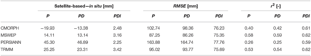
Table 5. Statistical indicators of CMORPH, MSWEP, PERSIANN, and TRMM precipitation vs. in situ data (average of 502 validation weather stations).

Hydrological Modeling and Discharge Evaluation

The daily precipitation datasets at 25 and 1 km resolutions (P, PD, and PDI) were used to force the OpenStreams wflow-hbv model. Previously, the model was calibrated and validated using in situ discharge data (Table S2). Further model calibration could have been done, but the idea was to fairly represent the main hydrological processes to assess the impact of various precipitation datasets and their spatial variability on simulated discharges.

Figure 7 shows simulated and observed discharge at La Esperanza station. The upstream area of this station is 13,508 km² (Table 3), which is covered by approximately 22 grid cells at 25 km resolution. As expected, discharge estimates when the model was driven with MSWEP and TRMM at 25 km resolution exhibit the highest agreement with observations. The lowest performance is provided when the model was forced with PERSIANN at 25 km resolution, with a significant discharge overestimation from April to September, in line with precipitation evaluation results. CMORPH results emphasize the limitations of this product for precipitation estimation in the basin, which tends to slightly underestimate discharge.

FIGURE 7

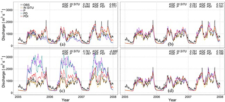
Figure 7. Daily observed discharge (black) and estimated discharge (orange, purple, blue, and red) time series at La Esperanza station (27037010) when the model was forced with (a) CMORPH, (b) MSWEP, (c) PERSIANN, and (d) TRMM for the 2005–2007 period. The orange lines represent discharge estimates when in situ precipitation data was used. The purple, blue, and red lines represent discharge estimates when satellite-based precipitation data was used at 25 km (P), at 1 km (PD), and at 1 km merged with in situ observations (PDI).

Driving the model with the downscaled precipitation datasets (PD and PDI) improves discharge simulation performance increasing KGE values. For MSWEP and TRMM (Figures 3b,d), the application of the downscaling procedure improves discharge estimates to a lesser extent (ΔKGE ~ 0.02) than when CMORPH (KGE ~ 0.10) and PERSIANN (KGE ~ 1.60) were used (Figures 3a,c). Due to the good model performance when MSWEP and TRMM datasets at 25 km resolution were used (KGE ~ 0.76), there are no significant discharge differences between using downscaled precipitation without (PD) and with (PDI) in situ observations. In this study, the spatial resolution of the hydrological model, 1 km, was finer compared to that of precipitation, 25 km. For hydrological models at 25 km resolution or coarser, it is expected that the precipitation downscaling procedure does not lead to further improvements on discharge estimates.

Figure 8 summarizes discharge simulation performances for the 22 gauging stations through boxplots of their KGE and r values when the model was forced with precipitation datasets at 25 km and 1 km resolutions (P, PD and PDI). KGE and r values obtained when the model was forced with precipitation datasets at 25 km resolution, P (purple) are lower than when in situ interpolated data was used (orange). Possible reasons could be the lower quality of satellite-based precipitation datasets compared to in situ data and that model parameters were calibrated with in situ precipitation data.

FIGURE 8

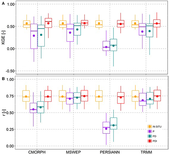
Figure 8. (A) KGE and (B) r values between daily simulated and observed discharge at the 22 discharge stations when the model was forced with in situ precipitation data (orange) and satellite-based precipitation datasets at 25 km (P, purple), at 1 km (PD, blue), and at 1 km merged with in situ observations (PDI, red) for the 2000–2012 period.

In agreement with precipitation results in Table 5, KGE and r increase when the downscaled precipitation PD was used (blue). This improvement is higher when the model was forced with downscaled precipitation merged with in situ observations, PDI (red). When analyzing the discharge performance obtained with PDI, the downscaling procedure manages to reduce the initial differences between the original MSWEP, TRMM, CMORPH, and PERSIANN precipitation datasets providing comparable averaged KGE (~0.57) and r (~0.75) values. These values are similar to those obtained when the model was forced with in situ data, KGE = 0.57 and r = 0.74 (except for PERSIANN).

Due to the application of the precipitation downscaling procedure, KGE increases were in the order of ~0.10–0.50 and correlation increases were in the order of ~0.02–0.40.

Once the impact of the downscaling procedure on discharge estimates was analyzed, the influence of the number of stations used in that procedure was further investigated. Figure 9 shows that when increasing the number of weather stations in the downscaling procedure, the performance of the hydrological model driven by the precipitation datasets improves. CMORPH precipitation is increased from ~110 to 200 mmm month⁻¹ and therefore, discharge is also increased from ~3,000 to 4,000 m³ s⁻¹. PERSIANN precipitation is reduced from ~260 to 180 mm month⁻¹ and therefore, discharge also decreases from ~7,000 to 4,500 m³ s⁻¹. In general, no further variations occur when increasing the number of weather stations above 100. The upstream area at Barbosa station is 228,192 km², hence 100 stations represent 2,282 km² per weather station average or a circle with a radius of ca. 27 km. A possible reason behind no further improvements when increasing the number of stations above 100 could be a value of decorrelation distance of precipitation larger than 27 km. Contrary to CMORPH and PERSIANN, MSWEP, and TRMM do not show a monotonic tendency to increase or decrease when the number of stations increases, as expected. Precipitation and discharge vary similarly until they reach constant values of ~190 mm month⁻¹ and 4,600 m³ s⁻¹, respectively (100 stations).

FIGURE 9

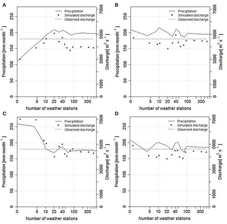
Figure 9. Monthly areal average precipitation (left vertical axis) and simulated (blue dots) and observed (green dashed line) average discharge (right vertical axis) at Barbosa station (25027530) at 1 km resolution for the 2000–2012 period, derived with different number of weather stations (0, 4, 8, 10, 20, 30, 40, 50, 60, 80, 100, 200, 400, and 616). (A) CMORPH, (B) MSWEP, (C) PERSIANN, and (D) TRMM. Logarithmic scale was used for the horizontal axis.

Figures 10, 11 summarizes KGE and r results for the 22 discharge stations when changing the number of weather stations in the precipitation downscaling procedure. Average values were calculated from KGE and r values obtained at all discharge stations.

FIGURE 10

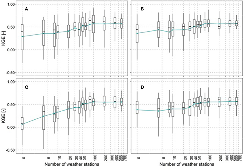
Figure 10. KGE values (y-axis) between daily simulated and observed discharge when the model was forced with (A) CMORPH, (B) MSWEP, (C) PERSIANN, and (D) TRMM precipitation datasets at 1 km resolution for the 2000–2012 period, derived with different number of weather stations (x-axis; 0, 4, 8, 10, 20, 30, 40, 50, 60, 80, 100, 200, 400, and 616). Logarithmic scale was used for the horizontal axis.

FIGURE 11

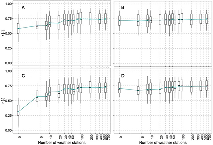
Figure 11. r values (y-axis) between daily simulated and observed discharge when the model was forced with (A) CMORPH, (B) MSWEP, (C) PERSIANN, and (D) TRMM precipitation datasets at 1 km resolution for the 2000–2012 period, derived with different number of weather stations (x-axis; 0, 4, 8, 10, 20, 30, 40, 50, 60, 80, 100, 200, 400, and 616). Logarithmic scale was used for the horizontal axis.

As expected, the lowest model performance was observed when downscaled precipitation was not merged with in situ data (with some exceptions for TRMM and MSWEP). In general, KGE and r values increase with increasing the number of weather stations in a monotonic tendency. KGE and r variation ranges differ between precipitation datasets. Average KGE values vary from 0.31 to 0.57 for CMORPH (Figure 10A) and from 0.07 to 0.55 for PERSIANN (Figure 10C). KGE and r values obtained when using MSWEP and TRMM show lower improvements when the number of stations increases, varying from 0.43 to 0.57 for MSWEP (Figure 10B) and from 0.39 to 0.57 for TRMM (Figure 10D). In spite of this general trend, sometimes the increase of the number of stations does not imply an increase in KGE and r values, or even causes a decrease. A possible reason behind this may be related to the inclusion of weather stations with lower quality data which would deteriorate the satellite-based precipitation datasets.

Increasing the number of stations above 100 did not further increase KGE or r values (the increase in average and median KGE and r values becomes relatively small).

Once the impact of increasing the number of weather stations for precipitation downscaling was analyzed, in situ precipitation values at the same samples of weather stations were interpolated (using the inverse distance weighting algorithm) to obtain different spatial maps at 1 km resolution. These maps, based only on in situ data, were used to force the hydrological model and discharge simulation performance results are shown in Figure 12.

FIGURE 12

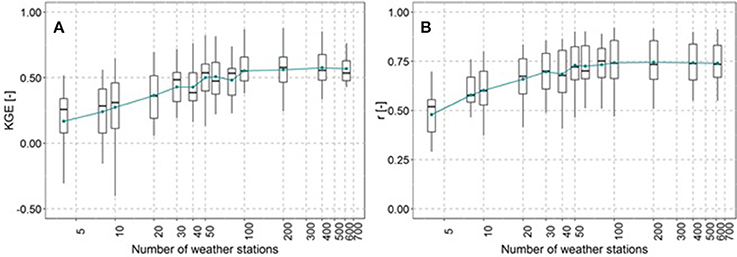
Figure 12. (A) KGE and (B) r values (y-axis) between daily simulated and observed discharge when the model was forced with in situ interpolated precipitation at 1 km resolution for the 2000–2012 period, derived with different number of weather stations (x-axis; 4, 8, 10, 20, 30, 40, 50, 60, 80, 100, 200, 400, and 616). Logarithmic scale was used for the horizontal axis.

As expected, increasing the number of weather stations used for in situ precipitation interpolation improves KGE (Figure 12A) and r (Figure 12B) values. Discharge simulation performance when the model was forced with downscaled precipitation is better than when the model was forced with in situ interpolated precipitation, considering the same weather station network. For example, for a network of 20 weather stations, higher KGE and r values were obtained when driving the model with downscaled MSWEP precipitation (KGE = 0.43 and r = 0.73) compared to those obtained when in situ interpolated precipitation was used (KGE = 0.36 and r = 0.66). This may be due to the downscaled datasets that better capture precipitation spatial variability combining different sources of information (satellite-based and in situ precipitation, vegetation response, elevation, slope, and aspect). These results show the potential of the described downscaling methodology for ungauged river basins or with limited number of rain gauge stations.

Discussion

Precipitation Downscaling and Evaluation

A new spatial downscaling procedure was developed and applied to four different satellite-based precipitation datasets to estimate precipitation at 1 km resolution in the Magdalena River basin in Colombia.

Firstly, satellite-based precipitation datasets at 25 km resolution were evaluated using in situ observations. Overall, results showed the great potential of all satellite-based precipitation data. As expected, MSWEP was the precipitation dataset with the best performance since this dataset is the result of combining several precipitation data sources, including gauge, satellite, and reanalysis data and therefore, it takes full advantage of the complementary nature of the different sources (Beck et al., 2017). Although CMORPH performance could be considered acceptable in terms of low RMSE and relatively high r² values, it tends to systematically underestimate precipitation for each month. Dinku et al. (2010) showed similar CMORPH results for Colombia and they partly attributed them to the orographic warm rain processes. PERSIANN shows the worst performance, which is consistent with previous studies in the area (de Goncalves et al., 2006; Ceccherini et al., 2015). Performance differences could be also due to the fact that CMORPH and PERSIANN do not include a posterior gauge correction, whereas MSWEP and TRMM do. Accompanying the satellite-based precipitation by an error product could benefit their use (Zeweldi and Gebremichael, 2009).

Secondly, a GWR model was used to downscale satellite-based precipitation from 25 to 1 km resolution using auxiliary information from vegetation response, elevation, slope, and aspect. Other regression methodologies, such as multiple linear regression or exponential regression (see overview in Table 1), could be used. However, the GWR model can capture the spatial variability in the relationship between precipitation, DEM, slope, aspect and EVI, which would not be noticed in the other regression models. GWR model parameters were downscaled using a cubic spline tension interpolator based on previous work by Ceccherini et al. (2015). Future studies might investigate alternative techniques, such as kriging or spatial autoregressive models. Additional variables, such as humidity, wind speed or topographical roughness, may be included as model predictors to further improve precipitation estimates. Moreover, a lag time of 1 month between precipitation and EVI was determined using average values over the entire basin. A spatial analysis of the correlation between precipitation and EVI with different lag times by regions may be done in the future, limiting the use of EVI predictor to those areas with higher correlations.

Thirdly, downscaled precipitation datasets were merged with in situ observations to take full advantage of all possible data sources available in the basin. When combining satellite and in situ observations, it is crucial to compare the rain gauge stations used in the derivation of TRMM and MSWEP with those locally available in the basin to derive independent downscaled precipitation datasets. Moreover, alternative interpolation techniques could be applied to interpolate the residuals between in situ and downscaled precipitation using auxiliary topographical information. Precipitation evaluation results are in line with those obtained by Duan and Bastiaanssen (2013) highlighting the importance of using the GWR model prior to the combination with in situ data to improve even further the accuracy of the final precipitation products.

To derive in situ precipitation maps at 1 km resolution, ground measurements at rain gauge stations were interpolated using the IDW algorithm. Various interpolation techniques were tested and IDW outperformed the other methods. In future studies, the non-homogeneous spatial distribution of stations in the basin may be analyzed in more detail and more sophisticated interpolation techniques could be investigated. Special attention should be paid to complex orographic areas in the south of the basin where the density of stations is lower.

The fractions of precipitation per day at 25 km were interpolated to a 1 km resolution to disaggregate precipitation from monthly to daily values, using an approach based on the downscaling methodology described by Duan and Bastiaanssen (2013). However, this approach might largely neglect the space-time correlation structure and the intermittent nature of rainfall, i.e., the fact that precipitation fields contain zeros in space and time. Alternative methodologies may be investigated to increase the temporal scale from monthly to daily.

Precipitation was evaluated to in situ observations during 2005–2012 period following a split-sample approach. This period represents fairly well the climate variability in the basin, however, longer data records could bring additional information to the study. Alternatively, a leave-one-out cross-validation procedure could be used to extend the study time period to 2000–2012 (Hunink et al., 2014). Moreover, additional performance indicators could be calculated to further analyze the impact of rain intensity, location and time errors, among others (Thiemig et al., 2012).

Satellite-based precipitation datasets were downscaled to 1 km resolution considering the complexity of the orography and precipitation patterns in the basin. Further investigation on the decorrelation distance at different temporal resolutions could give more information to face the challenge of matching spatial and temporal scale in precipitation monitoring.

Hydrological Modeling and Discharge Evaluation

To analyse the impact of precipitation spatial resolution on discharge estimates, in situ interpolated, non-downscaled, and downscaled precipitation datasets were used to force the OpenStreams wflow-hbv model. Previously, the hydrological model was calibrated with interpolated in situ precipitation data at 1 km resolution. Some previous studies calibrated the model for each precipitation dataset to evaluate the sensitivity of model parameters to precipitation (Andréassian et al., 2001; Nkiaka et al., 2017). In this study, model parameters are not optimized for each forcing aiming to avoid correcting precipitation errors through fine-tuning the hydrological processes representation in the model (sensitivity analysis).

Hydrological modeling results showed that precipitation spatial downscaling improves discharge estimates, not only in terms of reducing model bias, but also increasing model ability to capture the overall flow variability between extreme events, the timing and the shape of the hydrographs. Additional performance indicators could be calculated to extend the discharge evaluation, for example, by analyzing discharge peaks and recession periods. Precipitation datasets at intermediate spatial resolutions, such as 20, 15, 10, 5, or 2 km, could be derived and used to force the hydrological model to give some indications on appropriate spatial resolution for the determination of discharge (Lobligeois et al., 2014; Gascon et al., 2015). The impact of precipitation temporal resolution on simulated discharge may be additionally investigated. Various studies (Littlewood and Croke, 2008; Biemans et al., 2009; Ryo et al., 2014; Brauer et al., 2016) have shown that temporal effects in precipitation datasets, such as biases, may also have a deteriorating impact on discharge simulations. Moreover, investigating temporal downscaling to finer scales (3-hourly or hourly), could be of great added value for specific hydrological applications in the basin, such as extreme flood events in urban areas.

Downscaled satellite-based precipitation combined with in situ data lead to the highest improvement on discharge model performance. When increasing the number of rain gauges stations used in the downscaling procedure, discharge simulations improved in a monotonic tendency, with some exceptions where performance indicators even decreased. Previous studies (Bardossy and Das, 2008; Xu et al., 2013) have found similar results and attributed them to the contribution of individual weather stations and their location within the basin. Xu et al. (2013) explained that when a low number of stations is used, their location plays an important role. Although 10 stations cannot reproduce the spatial variability of precipitation in comparison with all 616 stations, if they would be more evenly spatially distributed within the basin that would significantly impact model results. A possibility for future research would be to further investigate the station networks that lead to a decrease in KGE and r values by regions, especially in mountainous areas where heavy orographic precipitation events occur, which highly contribute to discharge. Moreover, alternative sampling techniques could be used.

When analyzing the effect of the number of weather stations used in the downscaling procedure, results showed that no further improvements on discharge simulations were found when increasing the number of stations above 100. This gives an indication of the appropriate number of stations to accurately estimate discharge. Additional analysis could be done investigating, for example, the relative number of stations per unit of basin area, or inversely, the average area per weather station.

Discharge evaluation results are specific for this basin, hydrological model, precipitation datasets, and resolutions. The impact of the number of rain gauge stations and the spatial variability of precipitation on discharge simulations might differ depending on topography, soil type, basin hydrological characteristics and type of precipitation (Janis et al., 2004; Bardossy and Das, 2008). In the future, downscaled precipitation could be derived using the here-described approach (or an adaptation depending on in situ data availability) for a selection of basins around the world with diverse hydro-meteorological characteristics.

Overall, the new developed precipitation downscaling methodology showed great potential for hydrological modeling applications at a river basin scale. Future studies might consider using this downscaling procedure of satellite-based observations to derive an optimal precipitation product for accurate discharge simulations in ungauged river basins where scarce in situ data are available.

Conclusions

This study investigated how discharge estimates of a distributed hydrological model, OpenStreams wflow-hbv, can be influenced by precipitation spatial variability in the Magdalena River basin in Colombia. The effect of precipitation on discharge simulations was assessed by running the model with in situ and satellite-based precipitation datasets at non-downscaled and downscaled spatial resolutions. The conclusions of the study are as follows:

(i) At 25 km resolution, MSWEP and TRMM outperformed CMORPH and PERSIANN precipitation datasets.

(ii) The downscaling procedure resulted in highly improved accuracy of the four precipitation datasets. Vegetation, elevation, slope, and aspect were successfully used in a GWR model as proxies to precipitation leading to improvements of ~17% in RMSE, r² and bias compared to in situ observations. The combination with in situ precipitation data further improved them, due to the high density of weather stations in the basin. Lower density networks may limit the spatial correction impact, highlighting the significance of the GWR analysis in data-poor river basins.

(iii) Discharge model estimates were in better agreement with observations when MSWEP and TRMM were used to force the model compared to CMORPH and PERSIANN precipitation datasets at 25 km resolution.

(iv) Forcing the model with the downscaled precipitation datasets considerably improved discharge model estimates, with KGE increases in the order of 0.1 to 0.5.

(v) A higher number of weather stations was necessary in the downscaling procedure with in situ data of CMORPH and PERSIANN to achieve similar discharge performances than those obtained with MSWEP and TRMM. However, increasing the number of stations above 100 did not further improve model estimates with any precipitation dataset.

(vi) The downscaling of satellite-based precipitation datasets resulted in better discharge estimates compared to using only in situ precipitation data when using less than 100 weather stations.

Although results depend on the specifics of each basin, the present study showed that an accurate representation of precipitation spatial variability may help to improve discharge simulations. Downscaling procedures, such as the one used in this study, make globally available satellite-based precipitation datasets an interesting alternative/complement to ground data for hydrological modeling in poor-gauged or ungauged river basins.

Author Contributions

PL wrote most of the text, performed the analysis, and interpreted the validation of precipitation and discharge results. WI supported with the downscaling procedure, assisted in the analysis, and the text. ER supplied the ground precipitation and discharge measurements and supported with the local information of the basin and the model set up and analysis. GS supported with the text. JS supported with the model calibration and validation and assisted in the analysis and the text.

Funding

This research received funding from the European Union Seventh Framework Programme (FP7/2007-2013) under grant agreement no. 603608, Global Earth Observation for integrated water resource assessment: eartH2Observe. The contribution of WI was supported by the European Research Council (ERC) under the European Union's Horizon 2020 research and innovation programme (grant agreement number 676819) and the Netherlands Organization for Scientific Research under the Innovational Research Incentives Scheme VIDI (grant agreements 016.181.308).

Conflict of Interest Statement

JS is affiliated to the commercial company VanderSat based in the Netherlands and he does not have any competing or commercial interests associated to this paper. JS supported with the model calibration and validation and assisted in the analysis and the text.

The remaining authors declare that the research was conducted in the absence of any commercial or financial relationships that could be construed as a potential conflict of interest.

Acknowledgments

We would like to thank the Institute of Hydrology, Meteorology, and Environmental Studies (IDEAM) of Colombia for providing ground discharge and precipitation data. We would also like to thank Consiglio Nazionale delle Richerche (CNR) in Italy for providing the satellite-based precipitation datasets. We are very grateful to the Water Resources Research Group of National University of Colombia (GIREH) for their active support with the present research. We would also like to thank R. Hut, R. Uijlenhoet, and F. M. Pillosu who helped to improve our manuscript considerably.

Supplementary Material

The Supplementary Material for this article can be found online at: https://www.frontiersin.org/articles/10.3389/feart.2018.00068/full#supplementary-material

References

Adler, R. F., Kidd, C., Petty, G., Morissey, M., and Goodman, H. M. (2001). Intercomparison of global precipitation products: the third precipitation intercomparison project (PIP−3). Bull. Am. Meteorol. Soc. 82, 1377–1396. doi: 10.1175/1520-0477(2001)082<1377:IOGPPT>2.3.CO;2

CrossRef Full Text | Google Scholar

Andréassian, V., Perrin, C., Michel, C., Usart-Sanchez, I., and Lavabre, J. (2001). Impact of imperfect rainfall knowledge on the efficiency and the parameters of watershed models. J. Hydrol. 250, 206–223. doi: 10.1016/S0022-1694(01)00437-1

CrossRef Full Text | Google Scholar

Angarita, H., Delgado, J., Escobar-Arias, M. I., and Walschburger, T. (2013). “Escenarios de alteración regional del regimen hidrológico en la cuenca Magdalena-Cauca por intensificación de la demanda para hidroenergía,” in Conferencia Internacional Agua (Cali), 1–18.

Google Scholar

Arino, O., Ramos, J., Kalogirou, V., Defourny, P., and Achard, F. (2010). “GlobCover 2009,” in Proceedings of the Living Planet Symposium, SP-686 (Bergen), June 2010.

Google Scholar

Arnaud, P., Bouvier, C., Cisner, L., and Dominguez, R. (2002). Influence of rainfall spatial variability on flood prediction. J. Hydrol. 260, 216–230. doi: 10.1016/S0022-1694(01)00611-4

CrossRef Full Text | Google Scholar

Arnaud, P., Lavabre, J., Fouchier, C., Diss, S., and Javelle, P. (2011). Sensitivity of hydrological models to uncertainty in rainfall input. Hydrol. Sci. J. 56, 397–410. doi: 10.1080/02626667.2011.563742

CrossRef Full Text | Google Scholar

Bardossy, A., and Das, T. (2008). Influence of rainfall observation network on model calibration and application. Hydrol. Earth Syst. Sci. 12, 77–89. doi: 10.5194/hess-12-77-2008

CrossRef Full Text | Google Scholar

Beck, H. E., van Dijk, A. I., Levizzani, V., Schellekens, J., Miralles, D. G., Martens, B., et al. (2017). MSWEP: 3-hourly 0.25 global gridded precipitation (1979–2015) by merging gauge, satellite, and reanalysis data. Hydrol. Earth Syst. Sci. 21, 589–615. doi: 10.5194/hess-21-589-2017

CrossRef Full Text | Google Scholar

Bell, V. A., and Moore, R. J. (2000). The sensitivity of catchment runoff models to rainfall data at different spatial scales. Hydrol. Earth Syst. Sci. 4, 653–667. doi: 10.5194/hess-4-653-2000

CrossRef Full Text | Google Scholar

Berne, A., Delrieu, G., Creutin, J. D., and Obled, C. (2004). Temporal and spatial resolution of rainfall measurements required for urban hydrology. J. Hydrol. 299, 166–179. doi: 10.1016/S0022-1694(04)00363-4

CrossRef Full Text | Google Scholar

Biemans, H., Hutjes, R. W. A., Kabat, P., Strengers, B. J., Gerten, D., and Rost, S. (2009). Effects of precipitation uncertainty on discharge calculations for main river basins. J. Hydrometeorol. 10, 1011–1025. doi: 10.1175/2008JHM1067.1

CrossRef Full Text | Google Scholar

Bohnenstengel, S. I., Schlünzen, K. H., and Beyrich, F. (2011). Representativity of in situ precipitation measurements–A case study for the LITFASS area in North-Eastern Germany. J. Hydrol. 400, 387–395. doi: 10.1016/j.jhydrol.2011.01.052

CrossRef Full Text | Google Scholar

Boodoo, K. S., McClain, M. E., Upegui, J. J. V., and López, O. L. O. (2014). Impacts of implementation of Colombian environmental flow methodologies on the flow regime and hydropower production of the Chinchiná River, Colombia. Ecohydrol. Hydrobiol. 14, 267–284. doi: 10.1016/j.ecohyd.2014.07.001

CrossRef Full Text | Google Scholar

Bradley, A. V., Gerard, F. F., Barbier, N., Weedon, G. P., Anderson, L. O., Huntingford, C., et al. (2011). Relationships between phenology, radiation and precipitation in the Amazon region. Glob. Chang. Biol. 17, 2245–2260. doi: 10.1111/j.1365-2486.2011.02405.x

CrossRef Full Text | Google Scholar

Brauer, C. C., Overeem, A., Leijnse, H., and Uijlenhoet, R. (2016). The effect of differences between rainfall measurement techniques on groundwater and discharge simulations in a lowland catchment. Hydrol. Process. 30, 3885–3900. doi: 10.1002/hyp.10898

CrossRef Full Text | Google Scholar

Breusch, T. S., and Pagan, A. R. (1979). A simple test for heteroscedasticity and random coefficient variation. Econometr. J. Econometr. Soc. 47, 1287–1294. doi: 10.2307/1911963

CrossRef Full Text | Google Scholar

Camacho, L. A., Rodríguez, E., and Pinilla, G. (2008). “Modelación dinámica integrada de cantidad y calidad del agua del Canal del Dique y su sistema,” in XXIII Latinamerican Congress on Hydraulic (IARH) (Lagunar).

Ceccherini, G., Ameztoy, I., Hernández, C. P. R., and Moreno, C. C. (2015). High-resolution precipitation datasets in South America and West Africa based on satellite-derived rainfall, enhanced vegetation index and digital elevation model. Remote Sens. 7, 6454–6488. doi: 10.3390/rs70506454

CrossRef Full Text | Google Scholar

Chen, F., Liu, Y., Liu, Q., and Li, X. (2014). Spatial downscaling of TRMM 3B43 precipitation considering spatial heterogeneity. Int. J. Remote Sens. 35, 3074–3093. doi: 10.1080/01431161.2014.902550

CrossRef Full Text | Google Scholar

Chen, Y., Ebert, E. E., Walsh, K. J., and Davidson, N. E. (2013). Evaluation of TRMM 3B42 precipitation estimates of tropical cyclone rainfall using PACRAIN data. J. Geophys. Res. Atmosph. 118, 2184–2196. doi: 10.1002/jgrd.50250

CrossRef Full Text | Google Scholar

Collischonn, B., Collischonn, W., and Tucci, C. E. M. (2008). Daily hydrological modeling in the Amazon basin using TRMM rainfall estimates. J. Hydrol. 360, 207–216. doi: 10.1016/j.jhydrol.2008.07.032

CrossRef Full Text | Google Scholar

Cruz-Roa, A. F., Olaya-Marín, E. J., and Barrios, M. I. (2017). Ground and satellite based assessment of meteorological droughts: the Coello river basin case study. Int. J. Appl. Earth Observ. Geoinform. 62, 114–121. doi: 10.1016/j.jag.2017.06.005

CrossRef Full Text | Google Scholar

Dee, D. P., Uppala, S. M., Simmons, A. J., Berrisford, P., Poli, P., Kobayashi, S., et al. (2011). The ERA-Interim reanalysis: configuration and performance of the data assimilation system. Quart. J. R. Meteorol. Soc. 137, 553–597. doi: 10.1002/qj.828

CrossRef Full Text | Google Scholar

de Goncalves, L., Shuttleworth, W. J., Nijssen, B., Burke, E. J., Marengo, J. A., Chou, S. C., et al. (2006). Evaluation of model-derived and remotely sensed precipitation products for continental South America. J. Geophys. Res. Atmosph. 111:D16113. doi: 10.1029/2005JD006276

CrossRef Full Text | Google Scholar

Dinku, T., Connor, S. J., and Ceccato, P. (2010). “Comparison of CMORPH and TRMM-3B42 over mountainous regions of Africa and South America,” in Satellite Rainfall Applications for Surface Hydrology, eds M. Gebremichael and F. Hossain (Dordrecht: Springer), 193–204.

Google Scholar

DSMW (2007). Digital Soil Map of the World. Food and Agriculture Organization. Available online at: http://www.fao.org/geonetwork/srv/en/metadata.show?id=14116

Duan, Z., and Bastiaanssen, W. G. M. (2013). First results from Version 7 TRMM 3B43 precipitation product in combination with a new downscaling–calibration procedure. Remote Sens. Environ. 131, 1–13. doi: 10.1016/j.rse.2012.12.002

CrossRef Full Text | Google Scholar

Duan, Z., Bastiaanssen, W. G. M., and Liu, J. Z. (2012). “Monthly and annual validation of TRMM Multisatellite Precipitation Analysis (TMPA) products in the Caspian Sea Region for the period 1999–2003,” in Proceedings of International Geoscience and Remote Sensing Symposium (IGARSS) 2012, July 22–27 (Munich), 3696–3699.

Google Scholar

Durbin, J., and Watson, G. S. (1951). Testing for serial correlation in least squares regression. II. Biometrika 38, 159–177. doi: 10.2307/2332325

PubMed Abstract | CrossRef Full Text | Google Scholar

Emmanuel, I., Andrieu, H., Leblois, E., and Flahaut, B. (2012). Temporal and spatial variability of rainfall at the urban hydrological scale. J. Hydrol. 430, 162–172. doi: 10.1016/j.jhydrol.2012.02.013

CrossRef Full Text | Google Scholar

Ezzine, H., Bouziane, A., Ouazar, D., and Hasnaoui, M. D. (2017). Downscaling of open coarse precipitation data through spatial and statistical analysis, integrating NDVI, NDWI, elevation, and distance from sea. Adv. Meteorol. 2017:8124962. doi: 10.1155/2017/8124962

CrossRef Full Text | Google Scholar

Fang, J., Du, J., Xu, W., Shi, P., Li, M., and Ming, X. (2013). Spatial downscaling of TRMM precipitation data based on the orographical effect and meteorological conditions in a mountainous area. Adv. Water Resour. 61, 42–50. doi: 10.1016/j.advwatres.2013.08.011

CrossRef Full Text | Google Scholar

Fu, S., Sonnenborg, T. O., Jensen, K. H., and He, X. (2011). Impact of precipitation spatial resolution on the hydrological response of an integrated distributed water resources model. Vadose Zone J. 10, 25–36. doi: 10.2136/vzj2009.0186

CrossRef Full Text | Google Scholar

Funk, C., Peterson, P., Landsfeld, M., Pedreros, D., Verdin, J., Shukla, S., et al. (2015). The climate hazards infrared precipitation with stations—a new environmental record for monitoring extremes. Sci. Data 2:150066. doi: 10.1038/sdata.2015.66

PubMed Abstract | CrossRef Full Text | Google Scholar

Gascon, T., Vischel, T., Lebel, T., Quantin, G., Pellarin, T., Quatela, V., et al. (2015). Influence of rainfall space-time variability over the Ouémé basin in Benin. Proc. Int. Assoc. Hydrol. Sci. 368, 102–107. doi: 10.5194/piahs-368-102-2015

CrossRef Full Text | Google Scholar

Gessner, U., Naeimi, V., Klein, I., Kuenzer, C., Klein, D., and Dech, S. (2013). The relationship between precipitation anomalies and satellite-derived vegetation activity in Central Asia. Glob. Planet. Change 110, 74–87. doi: 10.1016/j.gloplacha.2012.09.007

CrossRef Full Text | Google Scholar

Goovaerts, P. (2000). Geostatistical approaches for incorporating elevation into the spatial interpolation of rainfall. J. Hydrol. 228, 113–129. doi: 10.1016/S0022-1694(00)00144-X

CrossRef Full Text | Google Scholar

Gupta, H. V., Kling, H., Yilmaz, K. K., and Martinez, G. F. (2009). Decomposition of the mean squared error and NSE performance criteria: implications for improving hydrological modelling. J. Hydrol. 377, 80–91. doi: 10.1016/j.jhydrol.2009.08.003

CrossRef Full Text | Google Scholar

Hou, A. Y., Kakar, R. K., Neeck, S., Ardeshir, A., Azarbarzin, A. A., Kummerow, C. D., et al. (2014). The global precipitation measurement mission. Bull. Am. Meteorol. Soc. 95, 701–722. doi: 10.1175/BAMS-D-13-00164.1

CrossRef Full Text | Google Scholar

Hoyos, N., Correa-Metrio, A., Sisa, A., Ramos-Fabiel, M. A., Espinosa, J. M., Restrepo, J. C., et al. (2017). The environmental envelope of fires in the Colombian Caribbean. Appl. Geogr. 84, 42–54. doi: 10.1016/j.apgeog.2017.05.001

CrossRef Full Text | Google Scholar

Hoyos, N., Escobar, J., Restrepo, J. C., Arango, A. M., and Ortiz, J. C. (2013). Impact of the 2010–2011 La Niña phenomenon in Colombia, South America: the human toll of an extreme weather event. Appl. Geogr. 39, 16–25. doi: 10.1016/j.apgeog.2012.11.018

CrossRef Full Text | Google Scholar

Hsu, K. L., Gao, X., Sorooshian, S., and Gupta, H. V. (1997). Precipitation estimation from remotely sensed information using artificial neural networks. J. Appl. Meteorol. 36, 1176–1190. doi: 10.1175/1520-0450(1997)036<1176:PEFRSI>2.0.CO;2

CrossRef Full Text | Google Scholar

Huete, A., Didan, K., Miura, T., Rodriguez, E. P., Gao, X., and Ferreira, L. G. (2002). Overview of the radiometric and biophysical performance of the MODIS vegetation indices. Remote Sens. Environ. 83, 195–213. doi: 10.1016/S0034-4257(02)00096-2

CrossRef Full Text | Google Scholar

Huffman, G. J., Adler, R. F., Bolvin, D. T., Gu, G., Nelkin, E. J., Bowman, K. P., et al. (2007). The TRMM multisatellite precipitation analysis (TMPA): Quasi-global, multiyear, combined-sensor precipitation estimates at fine scales. J. Hydrometeorol. 8, 38–55. doi: 10.1175/JHM560.1

CrossRef Full Text | Google Scholar

Hunink, J. E., Immerzeel, W. W., and Droogers, P. (2014). A high-resolution precipitation 2-step mapping procedure (HiP2P): development and application to a tropical mountainous area. Remote Sens. Environ. 140, 179–188. doi: 10.1016/j.rse.2013.08.036

CrossRef Full Text | Google Scholar

IDEAM (2017). Atlas Climatológico de Colombia (1981–2010). Available online at: http://atlas.ideam.gov.co/visorAtlasClimatologico.html (Accessed August 23, 2017).

Immerzeel, W. W., Quiroz, R. A., and De Jong, S. M. (2005). Understanding precipitation patterns and land use interaction in Tibet using harmonic analysis of SPOT VGT-S10 NDVI time series. Int. J. Remote Sens. 26, 2281–2296. doi: 10.1080/01431160512331326611

CrossRef Full Text | Google Scholar

Immerzeel, W. W., Rutten, M. M., and Droogers, P. (2009). Spatial downscaling of TRMM precipitation using vegetative response on the iberian peninsula. Remote Sens. Environ. 113, 362–370. doi: 10.1016/j.rse.2008.10.004

CrossRef Full Text | Google Scholar

Janis, M. J., Hubbard, K. G., and Redmond, K. T. (2004). Station density strategy for monitoring long-term climatic change in the contiguous United States. J. Clim. 17, 151–162. doi: 10.1175/1520-0442(2004)017<0151:SDSFML>2.0.CO;2

CrossRef Full Text | Google Scholar

Javanmard, S., Yatagai, A., Nodzu, M. I., BodaghJamali, J., and Kawamoto, H. (2010). Comparing high-resolution gridded precipitation data with satellite rainfall estimates of TRMM_3B42 over Iran. Adv. Geosci. 25, 119–125. doi: 10.5194/adgeo-25-119-2010

CrossRef Full Text | Google Scholar

Jia, S., Zhu, W., Lu, A., and Yan, T. (2011). A statistical spatial downscaling algorithm of TRMM precipitation based on NDVI and DEM in the Qaidam Basin of China. Remote Sens. Environ. 115, 3069–3079. doi: 10.1016/j.rse.2011.06.009

CrossRef Full Text | Google Scholar

Joyce, R. J., Janowiak, J. E., Arkin, P. A., and Xie, P. (2004). CMORPH: A method that produces global precipitation estimates from passive microwave and infrared data at high spatial and temporal resolution. J. Hydrometeorol. 5, 487–503. doi: 10.1175/1525-7541(2004)005<0487:CAMTPG>2.0.CO;2

CrossRef Full Text | Google Scholar

Karssenberg, D., Schmitz, O., Salamon, P., de Jong, K., and Bierkens, M. F. (2010). A software framework for construction of process-based stochastic spatio-temporal models and data assimilation. Environ. Model. Softw. 25, 489–502. doi: 10.1016/j.envsoft.2009.10.004

CrossRef Full Text | Google Scholar

Khan, S. I., Hong, Y., Gourley, J. J., Khattak, M. U. K., Yong, B., and Vergara, H. J. (2014). Evaluation of three high-resolution satellite precipitation estimates: potential for monsoon monitoring over Pakistan. Adv. Space Res. 54, 670–684. doi: 10.1016/j.asr.2014.04.017

CrossRef Full Text | Google Scholar

Koren, V. I., Finnerty, B. D., Schaake, J. C., Smith, M. B., Seo, D. J., and Duan, Q. Y. (1999). Scale dependencies of hydrologic models to spatial variability of precipitation. J. Hydrol. 217, 285–302. doi: 10.1016/S0022-1694(98)00231-5

CrossRef Full Text | Google Scholar

Kubota, T., Shige, S., Hashizume, H., Aonashi, K., Takahashi, N., Seto, S., et al. (2007). Global precipitation map using satellite-borne microwave radiometers by the GSMaP project: production and validation. IEEE Trans. Geosci. Remote Sens. 45, 2259–2275. doi: 10.1109/TGRS.2007.895337

CrossRef Full Text | Google Scholar

Langella, G., Basile, A., Bonfante, A., and Terribile, F. (2010). High-resolution space–time rainfall analysis using integrated ANN inference systems. J. Hydrol. 387, 328–342. doi: 10.1016/j.jhydrol.2010.04.027

CrossRef Full Text | Google Scholar

Levizanni, V., and Dorigo, W. A. (2017). D.3.7 – Release 3 of Finalized and Improved EO Datasets. Available online at: https://publicwiki.deltares.nl/display/INFORMED/D3.7+Release+3+of+Finalized+and+Improved+EO_Datasets (Accessed May 02, 2018).

Li, X. H., Zhang, Q., and Xu, C. Y. (2012). Suitability of the TRMM satellite rainfalls in driving a distributed hydrological model for water balance computations in Xinjiang catchment, Poyang lake basin. J. Hydrol. 426, 28–38. doi: 10.1016/j.jhydrol.2012.01.013

CrossRef Full Text | Google Scholar

Littlewood, I. G., and Croke, B. F. (2008). Data time-step dependency of conceptual rainfall—streamflow model parameters: an empirical study with implications for regionalisation. Hydrol. Sci. J. 53, 685–695. doi: 10.1623/hysj.53.4.685

CrossRef Full Text | Google Scholar

Lobligeois, F., Andréassian, V., Perrin, C., Tabary, P., and Loumagne, C. (2014). When does higher spatial resolution rainfall information improve streamflow simulation? An evaluation using 3620 flood events. Hydrol. Earth Syst. Sci. 18:575. doi: 10.5194/hess-18-575-2014

CrossRef Full Text | Google Scholar

Long, Y., Zhang, Y., and Ma, Q. (2016). A merging framework for rainfall estimation at high spatiotemporal resolution for distributed hydrological modeling in a data-scarce area. Remote Sens. 8:599. doi: 10.3390/rs8070599

CrossRef Full Text | Google Scholar

Loukas, A., and Vasiliades, L. (2014). Streamflow simulation methods for ungauged and poorly gauged watersheds. Nat. Haz. Earth Syst. Sci. 14, 1641–1661. doi: 10.5194/nhess-14-1641-2014

CrossRef Full Text | Google Scholar

Meng, J., Li, L., Hao, Z., Wang, J., and Shao, Q. (2014). Suitability of TRMM satellite rainfall in driving a distributed hydrological model in the source region of Yellow River. J. Hydrol. 509, 320–332. doi: 10.1016/j.jhydrol.2013.11.049

CrossRef Full Text | Google Scholar

Nash, J. E., and Sutcliffe, J. V. (1970). River flow forecasting through conceptual models part I—A discussion of principles. J. Hydrol. 10, 282–290. doi: 10.1016/0022-1694(70)90255-6

CrossRef Full Text | Google Scholar

Nkiaka, E., Nawaz, N. R., and Lovett, J. C. (2017). Evaluating global reanalysis datasets as input for hydrological modelling in the Sudano-Sahel region. Hydrology 4:13. doi: 10.3390/hydrology4010013

CrossRef Full Text | Google Scholar

Park, N. W. (2013). Spatial downscaling of TRMM precipitation using geostatistics and fine scale environmental variables. Adv. Meteorol. 2013, 1–9. doi: 10.1155/2013/237126

CrossRef Full Text | Google Scholar

QGIS. (2017). A Free and Open Source Geographic Information System. Available online at: http://www.qgis.org/en/site/ (Accessed August 21, 2017).

Quiroz, R., Yarlequé, C., Posadas, A., Mares, V., and Immerzeel, W. W. (2011). Improving daily rainfall estimation from NDVI using a wavelet transform. Environ. Model. Softw. 26, 201–209. doi: 10.1016/j.envsoft.2010.07.006

CrossRef Full Text | Google Scholar

Restrepo, J. D., Kettner, A. J., and Syvitski, J. P. (2015). Recent deforestation causes rapid increase in river sediment load in the Colombian Andes. Anthropocene 10, 13–28. doi: 10.1016/j.ancene.2015.09.001

CrossRef Full Text | Google Scholar

Restrepo, J. D., and Kjerfve, B. (2000). Magdalena river: interannual variability (1975–1995) and revised water discharge and sediment load estimates. J. Hydrol. 235, 137–149. doi: 10.1016/S0022-1694(00)00269-9

CrossRef Full Text | Google Scholar

Restrepo, J. D., and Syvitski, J. P. (2006). Assessing the effect of natural controls and land use change on sediment yield in a major Andean river: the Magdalena drainage basin, Colombia. AMBIO J. Hum. Environ. 35, 65–74. doi: 10.1579/0044-7447(2006)35[65:ATEONC]2.0.CO;2

PubMed Abstract | CrossRef Full Text | Google Scholar

Ryo, M., Saavedra Valeriano, O. C., Kanae, S., and Ngoc, T. D. (2014). Temporal downscaling of daily gauged precipitation by application of a satellite product for flood simulation in a poorly gauged basin and its evaluation with multiple regression analysis. J. Hydrometeorol. 15, 563–580. doi: 10.1175/JHM-D-13-052.1

CrossRef Full Text | Google Scholar

Sælthun, N. R. (1996). The Nordic HBV model. Norweg. Water Resour. Energy Admin. Publ. 7, 1–26.

Sangati, M., and Borga, M. (2009). Influence of rainfall spatial resolution on flash flood modelling. Nat. Haz. Earth Syst. Sci. 9, 575–584. doi: 10.5194/nhess-9-575-2009

CrossRef Full Text | Google Scholar

Schellekens, J. (2014). OpenStreams wflow Documentation Release 1.0RC1. Deltares. Available online at: http://wflow.readthedocs.org/en/latest/ (Accessed July 27, 2017).

Schellekens, J. (2016). OpenStreams Project: wflow Distributed Hydrological Modeling Platform. Available online at: https://github.com/openstreams/wflow (Accessed July 27, 2017).

Schellekens, J., and Weiland, F. S. (2017). Earth2observe/downscaling-tools: 2017. Delft: Pre-release.

Schuurmans, J. M., and Bierkens, M. F. P. (2006). Effect of spatial distribution of daily rainfall on interior catchment response of a distributed hydrological model. Hydrol. Earth Syst. Sci. Disc. 3, 2175–2208. doi: 10.5194/hessd-3-2175-2006

CrossRef Full Text | Google Scholar

Segond, M. L., Wheater, H. S., and Onof, C. (2007). The significance of spatial rainfall representation for flood runoff estimation: a numerical evaluation based on the Lee catchment, UK. J. Hydrol. 347, 116–131. doi: 10.1016/j.jhydrol.2007.09.040

CrossRef Full Text | Google Scholar

Shapiro, S. S., and Wilk, M. B. (1965). An analysis of variance test for normality (complete samples). Biometrika 52, 591–611.

Google Scholar

Shi, Y., and Song, L. (2015). Spatial downscaling of monthly TRMM precipitation based on EVI and other geospatial variables over the Tibetan Plateau From 2001 to 2012. Mountain Res. Devel. 35, 180–194. doi: 10.1659/MRD-JOURNAL-D-14-00119.1

CrossRef Full Text | Google Scholar

Sivapalan, M., Takeuchi, K., Franks, S. W., Gupta, V. K., Karambiri, H., Lakshmi, V., et al. (2010). IAHS Decade on Predictions in Ungauged Basins (PUB), 2003–2012: Shaping an exciting future for the hydrological sciences. Hydrol. Sci. J. 48, 857–880. doi: 10.1623/hysj.48.6.857.51421

CrossRef Full Text | Google Scholar

Smith, M. B., Koren, V. I., Zhang, Z., Reed, S. M., Pan, J. J., and Moreda, F. (2004). Runoff response to spatial variability in precipitation: an analysis of observed data. J. Hydrol. 298, 267–286. doi: 10.1016/j.jhydrol.2004.03.039

CrossRef Full Text | Google Scholar

Sun, G., Ranson, K. J., Kharuk, V. I., and Kovacs, K. (2003). Validation of surface height from shuttle radar topography mission using shuttle laser altimeter. Remote Sens. Environ. 88, 401–411. doi: 10.1016/j.rse.2003.09.001

CrossRef Full Text | Google Scholar

SWBD. (2017). Shuttle Radar Topography Mission Water Body Data. Available online at: https://dds.cr.usgs.gov/srtm/version2_1/SWBD/. More information can be found online at: https://lta.cr.usgs.gov/srtm_water_body_dataset (Accessed July 27, 2017).

Teng, H., Shi, Z., Ma, Z., and Li, Y. (2014). Estimating spatially downscaled rainfall by regression kriging using TRMM precipitation and elevation in Zhejiang Province, southeast China. Int. J. Remote Sens. 35, 7775–7794. doi: 10.1080/01431161.2014.976888

CrossRef Full Text | Google Scholar

Thiemig, V., Rojas, R., Zambrano-Bigiarini, M., Levizzani, V., and De Roo, A. (2012). Validation of satellite-based precipitation products over sparsely gauged African river basins. J. Hydrometeorol. 13, 1760–1783. doi: 10.1175/JHM-D-12-032.1

CrossRef Full Text | Google Scholar

Tramblay, Y., Bouvier, C., Ayral, P. A., and Marchandise, A. (2011). Impact of rainfall spatial distribution on rainfall-runoff modelling efficiency and initial soil moisture conditions estimation. Nat. Haz. Earth Syst. Sci. 11, 157–170. doi: 10.5194/nhess-11-157-2011

CrossRef Full Text | Google Scholar

Vischel, T., and Lebel, T. (2007). Assessing the water balance in the Sahel: impact of small scale rainfall variability on runoff. Part 2: idealized modeling of runoff sensitivity. J. Hydrol. 333, 340–355. doi: 10.1016/j.jhydrol.2006.09.007

CrossRef Full Text | Google Scholar

Wagener, T., Gupta, H., Yatheendradas, S., Goodrich, D., Unkrich, C., and Schaffner, M. (2007). Understanding Sources of Uncertainty in Flash-Flood Forecasting for Semi-arid Regions. Perugia: IAHS Publication.

Google Scholar

Weedon, G. P., Balsamo, G., Bellouin, N., Gomes, S., Best, M. J., and Viterbo, P. (2014). The WFDEI meteorological forcing data set: WATCH Forcing Data methodology applied to ERA-Interim reanalysis data. Water Resour. Res. 50, 7505–7514. doi: 10.1002/2014WR015638

CrossRef Full Text | Google Scholar

Weiland, F. S., Lopez, P., Van Dijk, A., and Schellekens, J. (2015). “Global high-resolution reference potential evaporation, in: MODSIM 2015,” in Conference Proceedings, Broadbeach (Broadbeach, QLD).

Google Scholar

Xu, G., Xu, X., Liu, M., Sun, A. Y., and Wang, K. (2015). Spatial downscaling of TRMM precipitation product using a combined multifractal and regression approach: demonstration for South China. Water 7, 3083–3102. doi: 10.3390/w7063083

CrossRef Full Text | Google Scholar

Xu, H., Xu, C. Y., Chen, H., Zhang, Z., and Li, L. (2013). Assessing the influence of rain gauge density and distribution on hydrological model performance in a humid region of China. J. Hydrol. 505, 1–12. doi: 10.1016/j.jhydrol.2013.09.004

CrossRef Full Text | Google Scholar

Zeweldi, D. A., and Gebremichael, M. (2009). Evaluation of CMORPH precipitation products at fine space–time scales. J. Hydrometeorol. 10, 300–307. doi: 10.1175/2008JHM1041.1

CrossRef Full Text | Google Scholar

Zhao, F., Zhang, L., Chiew, F. H., Vaze, J., and Cheng, L. (2013). The effect of spatial rainfall variability on water balance modelling for south-eastern Australian catchments. J. Hydrol. 493, 16–29. doi: 10.1016/j.jhydrol.2013.04.028

CrossRef Full Text | Google Scholar

Zoccatelli, D., Borga, M., Viglione, A., Chirico, G. B., and Blöschl, G. (2011). Spatial moments of catchment rainfall: rainfall spatial organisation, basin morphology, and flood response. Hydrol. Earth Syst. Sci. 15, 3767–3783. doi: 10.5194/hess-15-3767-2011

CrossRef Full Text | Google Scholar