Glacier Mass Changes of Lake-Terminating Grey and Tyndall Glaciers at the Southern Patagonia Icefield Derived From Geodetic Observations and Energy and Mass Balance Modeling

1. Introduction

1.1. Rationale

Most Patagonian glaciers have been thinning and retreating at high rates during the past decades. Mass loss of the Northern Patagonia Icefield (NPI) and the Southern Patagonia Icefield (SPI) contributed to sea-level rise by 0.042 ± 0.002 mm a⁻¹ between 1964/1975 and 2000 (Rignot et al., 2003), increasing to 0.067 ± 0.004 mm a⁻¹ between 2000 and 2012 (Willis et al., 2012b). The main driver of the long-term demise of the ice-fields is most likely to be the warming climate (e.g., Rignot et al., 2003; Sakakibara and Sugiyama, 2014). Observed annual air temperatures at surface stations have increased by + 0.04°C to + 1.4°C south of 46°S during the past century (Rosenblüth et al., 1995). No significant trend of precipitation has been observed since 1950, but large inter-annual and decadal variations have been found (Carrasco et al., 2008; Aravena and Luckman, 2009; Lenaerts et al., 2014). Reanalysis data from 1960 to 2000 however show a slight decrease in solid precipitation over the ice-fields as a result of increasing air temperatures (Rasmussen et al., 2007).

Despite the general retreat of the outlet glaciers of the NPI and SPI, the individual responses show spatial and temporal non-uniform patterns (e.g., Aniya et al., 1996; Rivera and Casassa, 1999; Rivera et al., 2007; Lopez et al., 2010; Davies and Glasser, 2012; Sakakibara and Sugiyama, 2014; Minowa et al., 2015; Malz et al., 2018). Recent retreats of calving glaciers, such as Upsala and Jorge Montt glaciers are associated with ice flow acceleration and ice dynamical thinning near the calving front (Naruse and Skvarca, 2000; Rivera et al., 2012; Jaber et al., 2013; Muto and Furuya, 2013; Sakakibara and Sugiyama, 2014; Mouginot and Rignot, 2015). However, only a small number of NPI and SPI outlet glaciers show an extraordinary retreat including a recent ice speed acceleration between 2000 and 2011. The mean ice speed of the NPI and SPI even decreased between 2000 and 2011 compared to the time period of 1984 to 2000 (Sakakibara and Sugiyama, 2014). The recent increase in mass loss of the NPI and SPI therefore still seems to be mainly caused by long-term warming, while fjord geometry and ice dynamic processes are responsible for the rapid frontal retreat of individual calving glaciers, which enhances the mass loss (Casassa et al., 1997; Koppes et al., 2011; Rivera et al., 2012; Willis et al., 2012a,b; Sakakibara and Sugiyama, 2014). Recent surface mass balance modeling studies, however, estimate positive surface mass balance for the NPI and SPI, suggesting a slight increase in precipitation and cooling of the upper-atmospheric temperatures during the last decade as being the main driver (Lenaerts et al., 2014; Schaefer et al., 2015; Mernild et al., 2016). The contrasting pattern of observed glacier retreat and positive surface mass balance are assumed to be a result of increasing ice flow velocities associated with ice loss due to calving. However, ice loss due to increasing ice flow velocities has been observed only for those few tide-water glaciers undergoing a recent rapid glacier change.

In this study we demonstrate how energy and mass fluxes vary in space and time for Grey and Tyndall glaciers at the SPI. We aim to compute high resolution 6-hourly fields of surface energy fluxes and climatic mass balance for two neighboring glacier catchments by applying the COupled Snowpack and Ice surface energy and MAss balance model (COSIMA) (Huintjes et al., 2015) between 2000 and 2016. Different statistical downscaling methods are used to derive atmospheric input datasets. Precipitation fields are generated by applying an orographic precipitation model (OPM hereafter) based on the linear theory of orographic precipitation by Smith and Barstad (2004). The model has also been implemented successfully in several previous glaciological studies (Schuler et al., 2008; Jarosch et al., 2012; Weidemann et al., 2013). Cloudiness patterns are obtained from MODIS satellite data product MOD10A1 to correct for spatial variations of solar radiation. Geodetic mass balance changes are obtained by subtracting high-resolution TanDEM-X and SRTM data between 2000 and 2014 (Malz et al., 2018). We derive frontal ablation from modeled climatic mass balance and geodetic mass balance for each glacier for the same study period. The paper focuses on the validation of the downscaling results of atmospheric input data, and the comparison of modeled surface energy-fluxes, modeled climatic mass balance, and derived frontal ablation between both study sites.

1.2. Study Area

The study sites Grey and Tyndall glaciers are located at the southeastern part of the SPI (50.7°S–51.30°S, 73.5°W–73.1°W) (Figure 1). In 2016, glacier areas were 239.0 and 301.4 km², respectively (Meier et al., 2018). The Equilibrium Line Altitude (ELA) is estimated to be 970 ± 50 m above sea level (a.s.l.) for Grey Glacier (De Angelis, 2014; Schaefer et al., 2015) and 925 ± 25 m a.s.l. for Tyndall Glacier (Nishida et al., 1995; De Angelis, 2014).

FIGURE 1

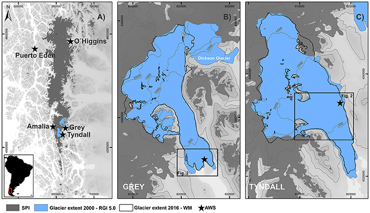
Figure 1. (A) The location of Grey and Tyndall glaciers at the SPI and the location of the weather stations Puerto Eden, O'Higgins, Amalia, Tyndall and Grey, (B) Grey Glacier including the location of AWS Grey, (C) Tyndall Glacier including the location of AWS Tyndall. Glacier outlines are visualized for 2000 based on the RGI 5.0 and for 2016 based on a new glacier inventory by Meier et al. (2018). The coordinates are in UTM zone 18S in meters.

Grey Glacier calves into a proglacial lake divided into three glacier termini which have shown different retreat and thinning rates over the last decades. The highest flow velocities of up to 2.8 m d⁻¹ are observed at the central front of the glacier (Schwalbe et al., 2017). The glacier front has remained rather stable over the past two decades. According to Davies and Glasser (2012), both glaciers showed similar annual shrinkage of about −0.1 to −0.15% (1970–2011), with the fastest period of area loss occurring from 1986 to 2001.

Information on accumulation amounts on the central part of the SPI are rare and mostly rely on a few firn cores retrieved of shallow to medium depth. The harsh weather conditions and the strong influence of meltwater percolation in the main plateaus are the prime reasons for sparse datasets (Godoi et al., 2002; Casassa et al., 2006). Three drilling sites located on the SPI allow estimation of a mean accumulation of 1.2 m water equivalent (w.e.) a⁻¹ at Perito Moreno at 2,000 m a.s.l. in 1980/81-1985/86 (Aristarain and Delmas, 1993), 12.9–14.7 m w.e. a⁻¹ at 1,756 m a.s.l. at Tyndall Glacier in 1998/99 with a firn-ice transition at 42.5 m depth (Godoi et al., 2002; Shiraiwa et al., 2002; Kohshima et al., 2007), and 3.4–7.1 m w.e. a⁻¹ at 2,600 m a.s.l. at Pio XI Glacier for the period 2000–2006 with a firn-ice transition at 50.6 m depth (Schwikowski et al., 2013). These observations suggest high spatial differences of accumulation in the upper part of the SPI, indicating also that these findings might be strongly influenced by local conditions at the drilling sites.

2. Data

2.1. Observations

Two automatic weather stations (AWS) are situated at Grey Glacier. AWS Grey has been running since March 2015 and measures hourly incoming solar radiation, wind speed and direction, air temperature, relative humidity at 2 m above the surface, and precipitation. Precipitation is measured at a height of 1 m using an unshielded tipping-bucket rain gauge. AWS Grey is located on rock close to the glacier margin between the eastern and middle front of Grey Glacier (Figure 1) at 50.98°S, 73.22°W at 229 m a.s.l. For modeling purpose, we installed an additional basic AWS in the ablation area at 50.97°S, 73.22°W for a period of 6 months from March 2015 to September 2015, measuring solar radiation, air temperature, and relative humidity. High coefficients of determination of 0.95–0.98 have been detected between the hourly datasets of both stations. To account for the cooling effect of the glacier surface we applied a bias-correction of air temperature as described in section 3.1.1.

The Chilean Water Directorate (DGA) provides additional AWS datasets within the study area. The AWS Tyndall is installed at 51.14°S, 73.35°W on the ablation area of Tyndall Glacier at 627 m a.s.l. and has been running since December 2013. This dataset contains hourly data of incoming and outgoing shortwave and longwave radiation, air temperature and humidity, surface pressure, wind speed and wind direction. Precipitation data of the weather stations Puerto Eden, O'Higgins, and Amalia are used for OPM validation. The weather stations Amalia and Puerto Eden are located west of the SPI at 50.95°S, 73.69°W at 60 m a.s.l. and 49.1°S, 74.4°W at 10 m a.s.l., while the weather station O'Higgins is situated at 48.91°S, 73.11°W at 265 m a.s.l. on the eastern margin of the SPI (Figure 1). Precipitation at Puerto Eden was measured from 1998 to 2010 although there are several data gaps. Data from the weather station O'Higgins covers the period from 2010 to 2014 while precipitation data from the weather station Amalia is limited to the period from June 2015 to April 2016.

Additionally, ablation stake measurements are available for Grey Glacier and Tyndall Glacier. Observations at Grey Glacier are limited to three time periods from January to March 2015, March to September 2015, and September 2015 to January 2016. Surface elevation changes of up to −8 m during the austral summer 2015/16 caused a complete melt-out of most stakes. Stake measurements were taken along a transect between 550 and 576 m a.s.l. on Tyndall Glacier from November 2012 to May 2013 (Geoestudios, 2013).

2.2. Reanalysis Data

Atmospheric model input datasets for COSIMA and OPM are derived from the latest large-scale ERA-Interim reanalysis product supplied by the European Centre for Medium-Range Weather Forecasts (ECMWF) (Dee et al., 2011).

COSIMA is forced by downscaled 6-hourly surface incoming solar radiation SW_in (W m⁻²) and air temperature T_2m (°C), as well as relative humidity rH_2m (%), surface pressure p_s (hPa), and wind speed at 2 m u_2m (m s⁻¹), derived from the grid point located closest to the study sites (51.0°S, 73.5°W) for the time period from April 1st, 2000 to March 31st, 2016.

Running the OPM to compute liquid P_liq and solid precipitation P_solid (m) requires the following 6-hourly ERA-Interim atmospheric datasets: horizontal and vertical wind components, temperature, relative humidity, geopotential heights, and large-scale precipitation. The environmental and moist adiabatic lapse rates are calculated using datasets of air temperatures from the 850 and 500 hPa levels. The wind components of the 850 hPa level are used as large-scale prevailing wind conditions. The data of precipitation and relative humidity (850 hPa) are needed to calculate the background precipitation and filter constraints within the OPM routine as described in section 3.1.3. Since the atmospheric input of the OPM should represent upstream conditions, data is averaged over six grid points located west along the SPI (50.0°S–53.0°S, 75°W–73.5°W).

2.3. Cloud Cover

Cloud cover information is required to correct the spatial distribution of incoming solar radiation. Binary cloud cover information is included by default in the daily MODIS (Moderate Resolution Imaging Spectroradiometer) snow cover product MOD10A1 Version 6 (Hall and Riggs, 2016) with a spatial resolution of 500 m. MOD10A1 has also been used successfully in previous studies over snow and ice-covered grounds (e.g., Möller et al., 2011; Spiess et al., 2016).

Daily fractional cloud cover is further derived by averaging the binary cloud cover information of a fixed 5 × 5 grid point window for each central grid point within the COSIMA modeling domain. This method is used to calculate fractional cloud cover in the MODIS product MOD06L2 and has also been customized for the MOD10A1 product by Möller et al. (2011). Fractional cloud cover information serves as COSIMA input for parametrization of the incoming and outgoing longwave radiation.

2.4. Elevation Data and Glacier Outline

The digital elevation model (DEM) generated from the Shuttle Radar Topography Mission (SRTM) (Hoffmann and Walter, 2006; Jarvis et al., 2008) is used as the reference surface elevation in 2000 for COSIMA and OPM runs. COSIMA and OPM runs are carried out with a spatial resolution of 500 and 1,000 m, respectively. Glacier outlines for model runs have been used from the Randolph Glacier Inventory RGI 5.0 for 2000 (Consortium, 2015) to compare COSIMA results with previous surface mass balance studies (Schaefer et al., 2015; Mernild et al., 2016). In the RGI 5.0 the catchment of Grey Glacier also includes the neighboring Dickson Glacier (Figure 1).

Mean annual surface height changes between 2000 and 2014 are derived from SRTM and TanDEM-X data (Malz et al., 2018). This data is further needed for geodetic mass balance and frontal ablation estimations. Furthermore, annual surface height changes are considered in the altitude dependent calculation of atmospheric variables, e.g., air temperature in COSIMA.

3. Methodology

3.1. Surface Energy and Mass Balance

Climatic mass balance changes are estimated using the open source COupled Snowpack and Ice surface energy and MAss balance model (COSIMA) that was designed and validated in detail by Huintjes et al. (2015). COSIMA combines a surface energy balance model with a multi-layer sub-surface snow and ice model to fully resolve energy fluxes and mass balance processes.

The energy balance model combines all energy fluxes F that contribute to the surface energy budget and calculates the energy available for surface melting Q_melt (Oerlemans, 2001):

$\begin{array}{rc}F=S{W}_{in}·(1-\alpha )+L{W}_{in}+L{W}_{out}+Q_{sens}+Q_{lat}+Q_g+Q_{liq}.& (1)\end{array}$

It takes into consideration: the shortwave incoming radiation SW_in, the albedo α, the incoming LW_in and outgoing longwave radiation LW_out, the sensible Q_sens and the latent heat flux Q_lat, the ground heat flux Q_g, and the heat flux of liquid precipitation Q_liq. The latter is normally neglected (Cuffey and Paterson, 2010) but has been included here due to the significant amount of liquid precipitation in the ablation area of Patagonian glaciers.

Ablation occurs due to sublimation, subsurface melt, and surface melt. Q_melt requires the surface temperature T_s to be at the melting point (0°C) and a positive energy flux F toward the surface to prevail. In this case, Q_melt equals F. If T_s is below the melting point, no melt occurs. The subsurface snow module is structured in layers of 0.2 m thickness with a domain depth of 100 m (Table 1). Each layer is characterized by a temperature, density and liquid water content. The densification of the dry-snow pack is calculated using an empirical relation according to Herron and Langway (1980). The initial density profile of the snow pack is calculated by a linear interpolation between 250 and 550 kg m⁻³. Different values of albedo for snow, firn and ice are considered (Table 1). A key variable to link the surface and subsurface modules is T_s since it controls the conductive heat flux between the surface and the two upper subsurface layers as well as defining LW_out and providing the lower temperature for calculating sensible and latent heat flux according to the bulk approach. Energy balance and subsurface heat conduction each provide T_s. Both modules are solved iteratively until the convergence of T_s. The initial subsurface temperature T_sub profile is linearly scaled from depth to the glacier surface between -1°C and 0°C (Table 1). In case modeled T_sub or T_s exceeds the melting point, it is set to 0°C and the remaining energy is used for subsurface or surface melt, respectively.

TABLE 1

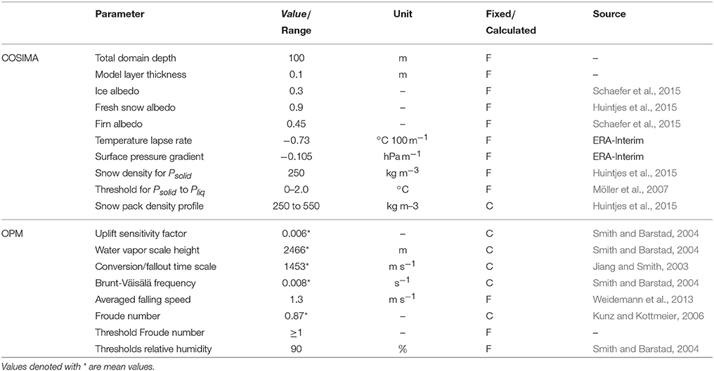
Table 1. Best-fit COSIMA and OPM parameter settings.

The parametrization of α is calculated as a function of snowfall frequency and snow depth following the scheme of Oerlemans and Knap (1998). The amount of incoming longwave radiation is parametrized from air temperature, water vapor pressure and cloud cover fraction while outgoing longwave radiation is calculated from the surface temperature using the Stefan-Boltzmann law, assuming an emissivity of one.

Turbulent heat fluxes Q_sens and Q_lat, are calculated through the bulk aerodynamic method according to Oerlemans (2001) between the surface and two meters above ground by means of T_2m, rH_2m and u_2m. Q_g describes the sum of conductive heat flux and the energy flux from penetrating shortwave radiation. Heat flux through liquid precipitation depends on the temperature differences between the surface and a height of 2 m and the amount of liquid precipitation (Maniak, 2010).

Melt water production at the glacier surface serves as input for the snow model to simulate percolation, retention and refreezing of melt water within the snow pack. COSIMA is described in more detail by Huintjes et al. (2015).

3.1.1. Air Temperature

Air temperature is statistically downscaled from ERA-Interim data to AWS Grey and AWS Tyndall by using Quantile Mapping (e.g., Panofsky and Brier, 1968; Gudmundsson et al., 2012). Quantile Mapping is a common technique for statistical bias correction of climate-model outputs by mapping the modeled cumulative distribution function of the variable of interest onto the observed cumulative distribution function that has been derived from empirical percentiles (Gudmundsson et al., 2012).

Bias-corrected air temperature is spatially interpolated using a fixed lapse rate from the AWS locations. The lapse rate is calculated from nine ERA-Interim grid points over the study area using monthly T_2m. Furthermore, the surface elevation is updated each mass balance year based on the mean annual surface elevation changes from 2000 to 2014 observed by Malz et al. (2018). Surface elevation changes since 2014 are then kept constant.

3.1.2. Solar Radiation

Incoming shortwave radiation SW_in is taken from ERA-Interim and downscaled to AWS data using Quantile Mapping. The spatial distribution of SW_in is derived from a modified radiation model according to Kumar et al. (1997) that computes clear-sky direct and diffuse shortwave radiation depending on the geographical position, elevation, albedo and shading by the surrounding terrain, and the slope and aspect of each grid cell. The potential clear-sky radiation SW_{in, pot, glacier} is corrected for cloud cover by downscaled ERA-Interim SW_{in, AWS} at the AWS grid point.

At each time step the ratio r_{SW, pot, glacier} of SW_{in, pot, AWS} at the AWS location and any other pixel SW_{in, pot, glacier} in the glacier domain is calculated. The spatial distribution of SW_{in, glacier} including the effects of cloud cover and terrain shading at each grid point is calculated by:

$\begin{array}{rc}S{W}_{in,glacier}=r_{SW,pot,glacier}·S{W}_{in,AWS}.& (2)\end{array}$

Equation (2) assumes a homogenous cloud cover over the glacier area. Since in reality the cloud cover varies between the AWS location and the upper parts of the glacier, an additional cloud cover correction factor is included. In cases when the cloud cover differs between the AWS location and any other location on the glacier, SW_{in, glacier} is calculated as follows:

$\begin{array}{rc}S{W}_{in,glacier,cloudy}=r_{SW,pot,glacier}·S{W}_{in,AWS}·\stackrel{\prime }{{\displaystyle \eta }}& (3)\end{array}$

$\begin{array}{rc}S{W}_{in,glacier,clear}=r_{SW,pot,glacier}·\frac{S{W}_{in,AWS}}{\stackrel{\prime }{{\displaystyle \eta }}}& (4)\end{array}$

Equation (3) corrects the distribution of incoming solar radiation glacier-wide in case of clear sky conditions at the AWS and cloudy conditions over the glacier, while Equation (4) is used in case of inverse conditions between AWS and the remaining parts of the glacier. $\acute{\eta }$ describes an empirical coefficient being 0.4 at 51°S (Budyko, 1974). The coefficient implies that during fully overcast conditions the clear-sky incoming shortwave radiation is reduced by 60%.

3.1.3. Precipitation

Precipitation distribution is modeled using an analytical orographic precipitation model (OPM) based on the linear steady-state theory of airflow dynamics (Smith and Barstad, 2004; Barstad and Smith, 2005). A more detailed description and validation of the model itself is given by Smith and Barstad (2004) and Barstad and Smith (2005) while the methodical application as used in this study is described in more detail in Weidemann et al. (2013).

The OPM estimates precipitation resulting from forced orographic uplift of air masses over a mountain assuming stable and saturated atmospheric conditions. The model estimates the condensation rate by the terrain-induced vertical air velocity, the horizontal wind speed and advection of water vapor, and includes effects of airflow dynamics and downslope evaporation as well. The main term of the linear model describing the orographic precipitation generation is solved in Fourier space for each Fourier component (k,l) as follows:

$\begin{array}{rc}\widehat{P}(k,l)=\frac{C_w·i·\sigma ·\widehat{h}(k,l)}{(1-i·m·H_w)(1+i·\sigma ·{\tau }_c)(1+i·\sigma ·{\tau }_f)}.& (5)\end{array}$

Equation (5) includes an uplift sensitivity factor C_w, the water vapor scale height H_w, the complex number i, the intrinsic frequency σ, the Fourier transform of the orography ĥ, and the vertical wavenumber m and the delay time scales for conversion τ_c and fallout τ_f of hydrometeors. The thermodynamic sensitivity C_w accounts for the effects of saturation water vapor density, the moist adiabatic and environmental lapse rates. H_w mainly depends on the environmental air temperature and lapse rate. Airflow dynamics are represented by the intrinsic frequency, including the vertical and horizontal winds. One of the airflow features included is the decay of vertical velocity with altitude which is described by m. The calculation of m contains the buoyancy frequency in saturated atmosphere and the moist Brunt-Väisälä frequency N_m to consider the effect of moist air masses on the static stability. Additionally, the precipitation generation is shifted downstream from the water source region depending on the wind speed and the cloud time parameter τ_c and τ_f.

The final term of orographic precipitation distribution is obtained by an inverse Fourier Transformation

$\begin{array}{rc}{P}_{oro}(x,y)=\int \int \widehat{P}(k,l)·e^{i·(kx+ly)}·dk·dl.& (6)\end{array}$

Final total precipitation fields are then generated by considering large-scale precipitation which we hereafter refer to as background precipitation P_back. The procedure of final precipitation and P_back calculations is described in the following.

The application of the OPM is limited to stable and saturated air masses, not capturing flow blocking effects or being applicable during unstable atmospheric conditions. Time intervals which do not fulfill the model constraints have to be filtered out. To ensure saturated and stable atmospheric conditions, relative humidity rH, N_m, and the moist Froude number are suitable as model constraints (e.g., Smith and Barstad, 2004; Schuler et al., 2008; Jarosch et al., 2012; Weidemann et al., 2013). The moist Froude number describes the airflow regime as a dimensionless number and can be associated to specific orographic precipitation patterns (Kunz and Kottmeier, 2006). In this study, it is used as an index to ensure linear airflow without flow blocking.

We need to run the OPM twice to replace the orographic fraction of ERA-Interim precipitation by high resolution orographic precipitation fields (e.g., Schuler et al., 2008; Weidemann et al., 2013). In the first step, the OPM is forced by ERA-Interim atmospheric and elevation data to determine P_back under consideration of the model constraints by subtracting the modeled orographic fraction from ERA-Interim precipitation. The second step implies the application of the OPM to the SRTM elevation model at a high spatial resolution of 1 km using the same input parameters to achieve high resolution P_oro fields. A threshold is applied to ensure positive values of P_oro. Finally, high-resolution total precipitation fields (P) are calculated by means of P_oro and P_back under consideration of the model constraints. In case model constraints are complied with, P_oro is added to P_back. Otherwise, only P_back is assumed.

The amount of solid precipitation P_solid is calculated by:

$\begin{array}{rc}{P}_{solid}=P·f,& (7)\end{array}$

$\begin{array}{rc}f=0.5·(-tanh((T_{2m}-1)·3)+1).& (8)\end{array}$

Applying Equation (7), the proportion of solid precipitation to total precipitation f is smoothly scaled between 100% and 0% within a T_2m range of 0°C and 2°C (Möller et al., 2007; Weidemann et al., 2013).

3.2. COSIMA-Calibration

As calibration for climatic mass balance results we use ablation stake measurements made at Grey Glacier from 2015/2016. We run COSIMA with varying parameter settings of model domain depth, layer depth, initial temperature profile, and albedo values for ice and snow based on values used in Huintjes et al. (2015) and Schaefer et al. (2015) to achieve the best model fit at the location of stakes for the measurement period. The RMSE between the best model fit and observed values is ±0.53 m w.e. COSIMA reproduces well the measured ablation amounts in winter and summer, as shown in Figure 2. In case of Grey Glacier, COSIMA tends to underestimate ablation. Best fit model parameters are listed in Table 1.

FIGURE 2

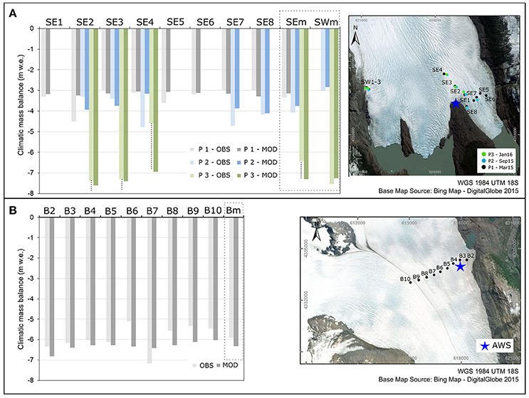
Figure 2. Comparison of modeled and observed climatic mass balance at Grey Glacier and Tyndall Glacier by means of ablation stake data. (A) Measurements at Grey Glacier were carried out three times: from January 2015 to March 2015 (P1), March 2015 to September 2015 (P2), and September 2015 to January 2016 (P3). SWm is the mean of measured ablation at the western glacier tongue and SEm mean values of the ablation at the eastern glacier tongue. The black dashed lines indicate that the observed surface mass balance values represent only minimum values since these stakes melted completely out over the austral summer 2015/16, (B) surface mass balance observations at Tyndall Glacier are available along a transect (B2-B10) from November 2012 to May 2013 (Geoestudios, 2013). Bm is the mean of measured ablation. The coordinates of the subset maps are in UTM zone 18S in meters.

Surface mass balance observations based on stake measurements at Tyndall Glacier from November 2012 to May 2013 are in good agreement with modeled climatic mass balance as well, with a RMSE of ±0.64 m w.e. COSIMA overestimates ablation in average by 6.5%.

3.3. COSIMA-Uncertainties

The uncertainties of modeled climatic mass balance are estimated by accounting for uncertainties in the spatial distribution of input datasets of air temperature and solid precipitation due to the lack of observations in the accumulation area. The spatial distribution of air temperature is determined by the chosen lapse rate, while the amount of modeled precipitation is mainly controlled by the OPM filter constraint rH. We therefore include varying values of these for the assessment of climatic mass balance uncertainties as described in the following section.

The best fit parameter setting based on our findings is listed in Table 1 including a calculated air temperature lapse rate of 0.73°C 100 m⁻¹ and a threshold for the OPM filter constraint rH of 90%. In addition, a second air temperature lapse rate of 0.67°C 100 m⁻¹—as used in earlier mass balance studies (e.g., Fernández and Mark, 2016)—and two rH thresholds of 85 and 95% are considered. In total, six runs are carried out for the mass balance year 2015/16 to assess the uncertainty of glacier-wide climatic mass balance and surface height change related to this climatic mass balance. This results in standard deviations of ±0.52 m w.e. and ±0.65 m w.e. for Grey Glacier and ±0.54 and ±0.67 m for Tyndall Glacier.

3.4. Geodetic Mass Balance Derived from TanDEM-X/SRTM

For DEM production, a differential SAR interferometric approach was used to generate a DEM out of bi-static TanDEM-X and TanSAR-X image pairs. Afterwards, the resulting DEM needed refined horizontal and vertical adjustments on the reference DEM (SRTM). Details about the interferometric processing and postprocessing can be found in detail in Malz et al. (2018).

After DEM generation, annual surface elevation changes were computed by differencing the TanDEM-X from the reference SRTM DEM for the time period between both acquisitions with a spatial resolution of 30 × 30 m. In this study, we further interpolated the final product to a spatial resolution of 500 m × 500 m as used in COSIMA to later derive the amount of frontal ablation. For both glaciers, surface height changes based on TanDEM-X/SRTM are converted to mass balance changes using a constant density of 850 kg m⁻³ (Huss, 2013) and to volume changes by multiplying with the pixel area (500 × 500 m).

We assess the uncertainties of elevation change rate dh/dt and mass balance M using a simplified error propagation of Malz et al. (2018). Mass balance uncertainty (ϵ_M) is estimated using:

$\begin{array}{rc}{ϵ}_M=\left|M\right|·\sqrt{\left(\frac{{\delta }_{dh/dt}}{dh/dt}\right)·\left(\frac{{\delta }_{\rho }}{\rho }\right)}& (9)\end{array}$

considering the uncertainty δ of elevation change rate dh/dt and of density ρ for mass conversion. The uncertainty of elevation change rate includes the error of the relative vertical accuracy of SRTM and TanDEM-X DEM, the radar penetration into snow and ice and an inaccuracy resulting from the extrapolation during gap filling Malz et al. (2018). For Grey and Tyndall glaciers, this results in δ_dh/dt of 0.19 and 0.24 m a⁻¹ for the study period of 2000–2014. A density uncertainty δ_ρ of 60 kg m⁻³ is taken into account while converting elevation changes to mass balance changes.

4. Results and Discussion

4.1. Atmospheric Data

The evaluation of COSIMA input based on ERA-Interim, downscaled ERA-Interim and MODIS is summarized in Table S1 for Grey and Tyndall glaciers for each mass balance year (April 1st to March 31). Results of downscaled air temperature, solar radiation and precipitation will be discussed in more detail in the following section. Annual glacier-wide means and standard deviations are given below for the study period of 2000 to 2016.

4.1.1. Air Temperature

Downscaling results of daily ERA-Interim T_2m by means of station data are visualized in Figure 3 for both AWS Grey and AWS Tyndall, respectively. Data from AWS Tyndall is split into a validation [April to October 2015 (yellow)] and calibration period. For the validation period, low temperatures are underestimated while high temperatures are overestimated.

FIGURE 3

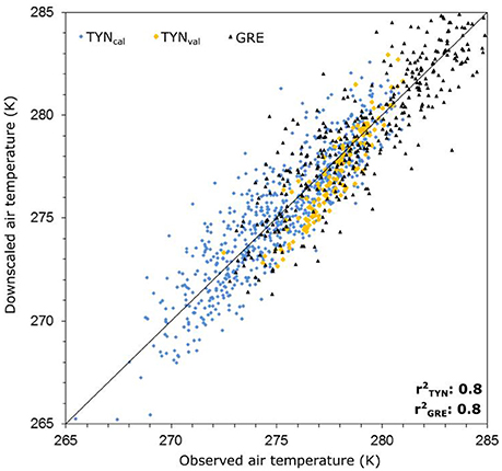
Figure 3. Downscaled ERA-Interim T_2m vs. observed data of AWS Grey (GRE) and AWS Tyndall (TYN). Data of AWS Tyndall from April to October 2015 (yellow) is used as validation.

The glacier-wide mean T_2m averaged over the whole study period is −2.4 ± 0.6°C for Grey Glacier and −0.7 ± 0.5°C for Tyndall Glacier. Glacier-wide air temperatures are higher than the mean value for the complete study period from 2003/04 to 2008/09 and 2011/12 to 2015/16. Air temperatures are lower than the average by 1.0°C to 1.3°C in 2001/02 and 2002/03. For the mass balance years 2004/05 to 2008/09, Mernild et al. (2016) simulates lower glacier-wide air temperatures of −2.7 ± 0.2°C and −1.0 ± 0.2°C compared to our results of −2.1 ± 0.2°C and −0.4 ± 0.2°C for Grey and Tyndall glaciers, respectively. For the time period of 2009/10 to 2013/14 both studies show slightly colder conditions.

4.1.2. Solar Radiation and Cloud Cover

SW_in of ERA-Interim and AWS Tyndall and AWS Grey are in good agreement with each other and achieve high correlation. The bias-correction based on Quantile Mapping as described earlier led to better results regarding the overall sums and maximal values. As shown in Figure 4 downscaled ERA-Interim data and observed data are in good agreement. The coefficient of determination is 0.8 for both AWS. Spatial fields of SW_in corrected by AWS data and MODIS cloud cover show an altitude-dependent pattern. The glacier-wide means of SW_in averaged over the study period are 109 ± 4 and 127 ± 5 W m⁻² for Grey and Tyndall glaciers respectively (Table S1).

FIGURE 4

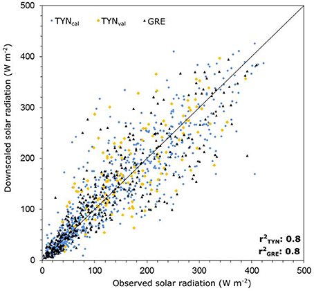
Figure 4. Downscaled ERA-Interim SW_in vs. observed data of AWS Grey (GRE) and AWS Tyndall (TYN). Data of AWS Tyndall from April to October 2015 (yellow) is used as validation.

Cloud cover patterns by MODIS10A1 show overcast conditions during 90% of the time at the upper parts of both glaciers. Mean cloud cover is less in the lower parts with values ranging from 55 to 80%. The glacier-wide mean is 85 ± 0.1% for Grey Glacier, while overcast conditions at Tyndall Glacier occur 79 ± 0.1 % of the time.

4.1.3. Precipitation

OPM runs have been carried out with varying thresholds of the model constraint rH according to the values used in previous studies (e.g., Crochet et al., 2007; Schuler et al., 2008; Jarosch et al., 2012) to find the best model fit compared to observed data. We chose the measurement period from AWS Grey from April 2015 to March 2016 to be the calibration period and, the available data from AWS Grey and the weather station Amalia to be the calibration data. Best fits have been achieved using the constraint rH≥90 which has also been applied successfully at the Gran Campo Nevado Ice Cap by Weidemann et al. (2013). For the given constraints, the OPM performs 55% of the time.

Best-fit OPM results are compared to observed precipitation data from four weather stations as illustrated in Figure 5. The explained variance between modeled and observed monthly precipitation data are 64% for the stations Puerto Eden, Amalia, and O'Higgins, and 73% for AWS Grey. The amount of modeled orographic precipitation accounts for 79.7 and 41.2% of the total modeled precipitation amount for the weather station Amalia and the AWS Grey, respectively. The weather stations Puerto Eden and O'Higgins are less influenced by orographic effects (orographic fraction less than 15%) due to the larger distance to the mountain range leading to a small fraction of modeled orographic precipitation. At these locations, modeled precipitation is mainly determined by the modeled background precipitation, which is based on ERA-Interim precipitation. The annual amounts of ERA-Interim precipitation are reduced by up to 15% in the central parts of the mountain range after subtracting the modeled orographic fraction from ERA-Interim precipitation as part of the background precipitation calculation.

FIGURE 5

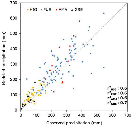
Figure 5. Monthly modeled precipitation (mm) by OPM simulations and observed precipitation of the weather stations Puerto Eden (PUE), O'Higgins (HIG), Amalia (AMA), Tyndall (TYN), and Grey (GRE).

Varying the filter constraint rH determines the amount of modeled orographic precipitation which is either reduced or enhanced. Therefore, this affects in particular the modeled precipitation at the locations of the weather station Amalia and the AWS Grey, which are highly influenced by orographic effects. Mean annual modeled precipitation amounts increase by 3–6% using rH≥85 at the four weather stations, while they decrease by 2–14% using rH≥95. Maximal annual precipitation amounts are in general shifted slightly to the windward side of the SPI mountain range. Depending on the filter constraints, the maximal annual precipitation amounts differ by around ±15% compared to rH≥90.

In general, the OPM tends to overestimate precipitation amounts at the weather stations. Despite possible measurement inaccuracies, the results are still in good agreement with observed data. Precipitation measuring equipment, such as installed at Grey Glacier, tends to underestimate precipitation in cases of snowfall or high wind speeds.

The glacier-wide mean annual precipitation amounts are 5.9 ± 1.0 m w.e. a⁻¹ at Grey Glacier and 7.1 ± 1.1 m w.e. a⁻¹ at Tyndall Glacier, averaged over the study period of 2000–2016. Mernild et al. (2016) simulate glacier-wide annual precipitation amounts of 10.26 ± 0.54 m w.e. a⁻¹ for Grey Glacier and 9.19 ± 0.46 m w.e. a⁻¹ for Tyndall Glacier between 2004/05 and 2013/14. These values are significantly higher than our findings. For the same period, we simulate glacier-wide mean annual precipitation of 6.27 ± 1.0 m w.e. a⁻¹ for Grey Glacier and 7.45 ± 1.1 m w.e. a⁻¹ for Tyndall Glacier.

The modeled ratio of solid to overall precipitation accounts for about 84.5 and 69.5% for Grey and Tyndall glaciers, respectively. Mean values for the SPI are estimated between 55% (Mernild et al., 2016) and 59% (Schaefer et al., 2015). Higher ratios of solid to overall precipitation for Grey and Tyndall glaciers compared to the mean value for the SPI seem reasonable since more than about 80% of the total falls in higher elevations as solid precipitation. This is at least partly due to the southern and lee-side location of these glaciers within the SPI.

4.2. Modeled Surface Energy Balance

The glacier-wide mean monthly surface energy balance components for both glaciers averaged between 2000 and 2016 are shown in Figure 6. The glacier-wide energy input is dominated year-around by LW_in (+ 279 W m⁻²) and SW_in (+ 109 W m⁻²), followed by Q_sens (+ 11 W m⁻²), Q_g (+ 4 W m⁻²) and Q_liq (+ 1 W m⁻²). Available energy at the glacier surface is consumed by LW_out (-288 W m⁻²), SW_out (−70 W m⁻²), Q_lat (−9 W m⁻²), and Q_melt (−36 W m⁻²). The main source of melt energy is SW_net (+ 39 W m⁻²).

FIGURE 6

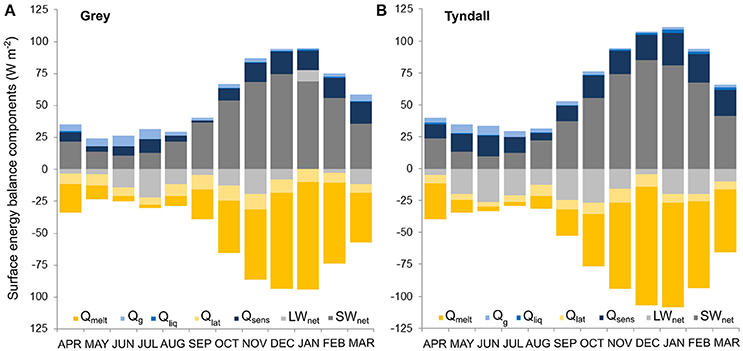
Figure 6. Monthly surface energy balance components averaged between April 2000 and March 2016 for (A) Grey Glacier and (B) Tyndall Glacier. Abbreviations are explained in Equation 1.

The highest SW_net values are reached during the summer months (October to March) due to higher incoming solar radiation. Albedo values are similar throughout the year with a glacier wide-mean of 0.6. The highest values of Q_sens are reached during the austral summer months while Q_g is slightly higher during the winter. LW_in exceeds the amount of LW_out in January over extensive areas of the glacier and air temperatures are above the melting point and relative humidity is high in January. This atmospheric situation results in a large down-welling long-wave radiation from the atmosphere toward the glacier surface. The glacier and snow emission, however, are restricted to emission at 0°C. Therefore, LW_out is limited to 311 W m⁻². In consequence, the model calculates positive LW_net for the core melt phase in the austral summer.

Q_liq is negligible regarding the glacier-wide mean. However, it plays a more prominent role as a source of melt energy in the ablation area. Positive Q_g may result due to the assumption of the ice temperature at the bottom of the model domain section (3.1), which may lead to unrealistic high positive Q_g values especially at higher elevation where the annual air temperature is lower.

The energy budget of a snowpack is also affected by snow drift. Since COSIMA does not integrate snow drift parametrization, sublimation at the glacier surface may be overestimated (Barral et al., 2014; Huintjes et al., 2015). Furthermore, katabatic flow over large glaciers generates turbulences and enhances the turbulent exchange (Q_lat, Q_sens) (Oerlemans and Grisogono, 2002). Surface melt may therefore be underestimated by neglecting katabatic winds when applying COSIMA.

The surface energy balance components of Tyndall Glacier do not show any significant differences compared to Grey Glacier between 2000 and 2016. The glacier-wide energy input is also dominated by LW_in (+ 273 W m⁻²) and SW_in (+ 127 W m⁻²), followed by Q_sens (+ 16 W m⁻²), Q_g (+ 3 W m⁻²) and Q_liq (+ 1 W m⁻²). Energy sinks are LW_out (-291 W m⁻²), SW_out (-82 W m⁻²), Q_lat (−7 W m⁻²), and Q_melt (-40 W m⁻²). The modeled radiation terms at the AWS Tyndall pixel are in good agreement with observed data. The overall mean of SW_in, SW_out, LW_in, and LW_out differ by 5–7% for the mass balance year of 2015/16.

4.3. Modeled Climatic Mass Balance

Modeled glacier-wide mean annual climatic mass balance are positive for Grey Glacier with +0.86 ± 0.52 m w.e. a⁻¹ and for Tyndall Glacier with +0.41 ± 0.54 m w.e. a⁻¹ for the study period from April 2000 to March 2016 (Table S2).

Negative climatic mass balance years of Grey Glacier are simulated for 2001/02, 2004/05, 2011/12, and 2015/16, while the most negative climatic mass balance is reached in 2015/16 (Table S2). In mass balance years where the climatic mass balance is negative, either less P_solid, higher T_2m, or higher SW_in amounts occurred compared to the average (Figure 7). High positive climatic mass balance years are modeled for 2007/08 and 2013/14 caused by above-average P_solid amounts and lower SW_in values. Very low mean T_2m compensate low amounts of P_solid and SW_in in 2000/01. The glacier-wide mean climatic mass balance for the period 2000–2016 ranges from −11.9 ± 2.1 m w.e. a⁻¹ in the lowest areas of the ablation area to + 10.3 ± 1.8 m w.e. a⁻¹ in the top parts of the accumulation area (Figures 8, 9).

FIGURE 7

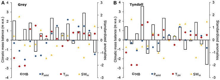
Figure 7. Modeled annual climatic mass balance (MB) based on COSIMA simulations and standardized anomalies of P_solid, T_2m, SW_in from the mean between April 2000 and March 2016 for (A) Grey Glacier and (B) Tyndall Glacier.

FIGURE 8

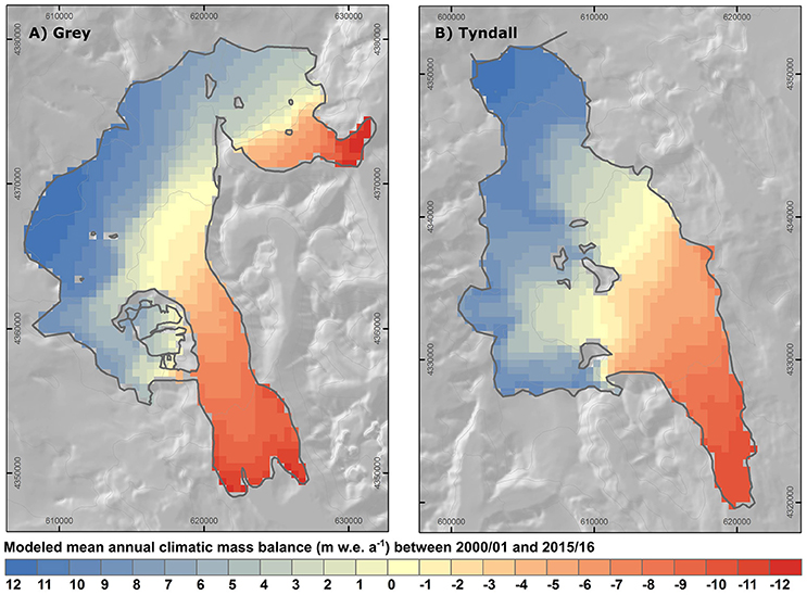
Figure 8. Modeled mean annual climatic mass balance in m w.e. a⁻¹ based on COSIMA simulations for the study period April 2000 to March 2016 for (A) Grey Glacier and (B) Tyndall Glacier. The coordinates are in UTM zone 18S in meters.

FIGURE 9

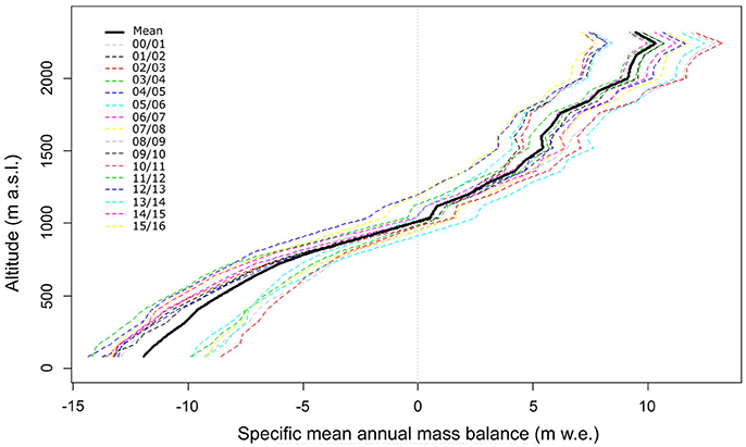
Figure 9. Modeled climatic mass balance profiles for Grey Glacier for each mass balance year from 2000/2001 (00/01) to 2015/2016 (15/16). Climatic mass balance is averaged over 80 m altitude bins.

Modeled mean annual ELA accounts for 960 ± 70 m a.s.l. ranging from 900 to 1,140 m a.s.l. These values are in good agreement with estimated mean ELA of De Angelis (2014) and Schaefer et al. (2015). The highest values for ELA of up to 1,140 m a.s.l. are simulated for the climatic mass balance years 2004/05 and 2015/2016. According to Malz et al. (2018), larger surface lowering have been observed at both outer glacier tongues of Grey Glacier. This pattern can also be distinguished in the modeled climatic mass balance results mainly because of the elevation feedback in air temperature as a consequence of the fact that the lateral glacier tongues have a lower surface elevation than Grey Glacier's middle branch (Figure 8).

For Tyndall Glacier, negative climatic mass balance is simulated in 2001/02, 2004/05, 2006/07, 2011/12, 2012/13, 2014/5, and 2015/16 (Table S2). The inter-annual variations of climatic mass balance are high, ranging from −2.60 ± 0.54 to +3.60 ± 0.54 m w.e. a⁻¹. In positive climatic mass balance years higher P_solid, lower T_2m, or lower SW_in amounts occurred compared to the average of each variable (Figure 7). Very high positive climatic mass balance in 2003/2004 is caused by high solid precipitation amounts in the lower altitudes. The combination of high air temperatures, high incoming solar radiation, and low solid precipitation amounts caused the strongly negative mass balance year in 2015/16.

The glacier-wide mean climatic mass balance for the period 2000–2016 ranges from −10.9 ± 3.2 m w.e. a⁻¹ in the lowest areas of the ablation area to +11.4 ± 1.9 m w.e. a⁻¹ in the top parts of the accumulation area. In some years modeled annual ablation is as negative as −13.5 m w.e. a⁻¹ and maximum accumulation reaches up to + 14.7 m w.e. a⁻¹ (Figure 10). The amount of accumulation in the highest altitudes seems reasonable compared to the study of Kohshima et al. (2007) who estimated an annual net accumulation in the period of the austral winter 1998 to the austral winter 1999 of + 12.9 m w.e. at 1,756 m a.s.l. The mean modeled ELA is 920 ± 60 m a.s.l. ranging from 760 m a.s.l. to 1,000 m a.s.l. ELA values are within the range of previous estimates by Nishida et al. (1995), Casassa et al. (2014), and De Angelis (2014).

FIGURE 10

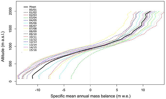
Figure 10. Modeled climatic mass balance profiles for Tyndall Glacier for each mass balance year from 2000/2001 (00/01) to 2015/2016 (15/16). Climatic mass balance is averaged over 80 m altitude bins.

Comparing modeled climatic mass balance results with previous studies, especially Mernild et al. (2016), we simulate less positive climatic mass balance including high year to year variations. According to Mernild et al. (2016), mean annual surface mass balance was estimated to be about +2.86 ± 0.28 and +0.71 ± 0.35 m w.e. a⁻¹ between 2004/05 to 2008/2009 for Grey and Tyndall glaciers, respectively, with a slight increase in positive surface mass balance for the following period between 2009/10 and 2013/2014. COSIMA climatic mass balance results for the period 2004/05 to 2008/09 are less positive with +0.67 ± 0.52 m w.e. for Grey Glacier and +0.35 ± 0.54 m w.e. a⁻¹ for Tyndall Glacier. The increase in positive climatic mass balance for the following period to 2013/14 is also reproduced by COSIMA. The contributions of subsurface melt, sublimation, refreezing, and evaporation are comparatively small (Table S2). The amounts of sublimation and evaporation are similar to values of Mernild et al. (2016).

The main reason for the differences in climatic mass balance is the amount of modeled annual precipitation. Current estimates from Schaefer et al. (2013); Lenaerts et al. (2014); Mernild et al. (2016) based on numerical simulations suggest average accumulation rates of 8-9 m w.e. a⁻¹ for the SPI. At isolated locations, extreme precipitation rates of up to 30 m w.e. a⁻¹ are suspected. These rather unrealistic amounts may result from an overestimation of modeled water vapor over the SPI. However, the lack of observed accumulation data of the SPI as described in section 1.2 and especially at Grey and Tyndall glaciers does not allow a detailed validation of modeled precipitation amounts.

4.4. Observed Geodetic Balance and Derived Frontal Ablation

Glacier-wide mean annual surface height changes between 2000 and 2014 simulated by COSIMA show an overall increase of +2.34 ± 0.65 m a⁻¹ for Grey Glacier and +1.93 ± 0.67 m a⁻¹ Tyndall Glacier due to high accumulation amounts. Observed mean annual surface height changes based on TanDEM-X/SRTM data indicate glacier average ice thinning of -1.23 ± 0.19 m a⁻¹ and −3.04 ± 0.24 m a⁻¹ for Grey and Tyndall glaciers, respectively. Figure 11 illustrates the spatial differences of surface height changes between COSIMA and TanDEM-X/SRTM, interpolated to 500 m, for both glaciers. TanDEM-X/SRTM observes glacier thinning even in the accumulation areas, while COSIMA estimates a gain of mass in the accumulation area and a loss of mass in the ablation area (Figure 12).

FIGURE 11

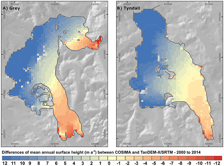
Figure 11. Differences between mean annual surface height changes (m) based on COSIMA as the result of climatic mass balance and mean annual surface height changes (m) based on TanDEM-X/SRTM, interpolated to a spatial resolution of 500 m, between 2000 and 2014 for (A) Grey Glacier and (B) Tyndall Glacier. The coordinates are in UTM zone 18S in meters.

FIGURE 12

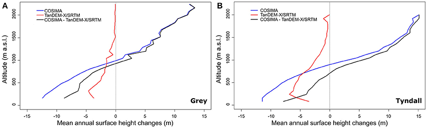
Figure 12. Profiles of differences between mean surface height changes (m) based on COSIMA as the result of climatic mass balance and mean annual surface height changes (m) based on TanDEM-X/SRTM for (A) Grey Glacier and (B) Tyndall Glacier. Differences are averaged over 80 m altitude bins.

The spatial distribution of surface height at the glacier fronts of Grey are non-uniform. Differences between both datasets at the outer tongues are small, especially at the western part, while high differences occur at the middle part of Grey Glacier. The latter is caused by a constant ice flow into this branch over time. Surface height changes and the front position of this middle branch remain constant over the entire study period. The western and eastern branches of the glacier tongue, however, seem to be partially decoupled from the main ice flow causing surface lowering which is mainly driven by climatic mass balance processes. The different ice dynamical effects at the glacier fronts are underlined by observed ice velocities based on LandSat-8 by Schwalbe et al. (2017). The highest velocities are observed at the middle part of the glacier terminus while the ice flow within the outer fronts is smaller. At Tyndall Glacier, we observe a more uniform pattern at the front but also a retreat of the glacier front (Figure 11). As expected, the smallest differences of surface height changes between COSIMA and TanDEM-X/SRTM are close to the mean ELA of both glaciers (Figure 12).

The glacier-wide mean annual climatic mass balance by COSIMA for the period of 2000–2014 is +1.02 ± 0.52 m w.e.a⁻¹ and +0.68 ± 0.54 m w.e.a⁻¹ for Grey and Tyndall glaciers, respectively. The positive climatic mass balance is mainly influenced by high accumulation amounts in the upper parts of the glaciers. A significant increase of glacier mass in the accumulation area has not been observed by TanDEM-X/SRTM (Figure 12).

Converting surface height changes by TanDEM-X/SRTM into mass balance changes yields in a mean geodetic mass balance of −1.05 ± 0.18 m w.e.a⁻¹ for Grey Glacier and −2.58 ± 0.28 m w.e.a⁻¹ for Tyndall Glacier. Since different densities for snow, firn, and ice are used within COSIMA, the mean density for converting surface height changes into climatic mass balance changes is lower within the COSIMA model than the density of 850 kg m⁻³ assumed for converting observed surface height changes by TanDEM-X/SRTM.

The differences between the modeled climatic mass balance and the geodetic mass balance are assumed to equal the amount of ice loss by frontal ablation which accounts for 2.07 ± 0.70 m w.e. a⁻¹ for Grey Glacier and 3.26 ± 0.82 m w.e. a⁻¹ for Tyndall Glacier. Ice loss by surface melt is larger than by frontal ablation with mean annual amounts of 3.48 m w.e.a⁻¹ and 3.71 m w.e.a⁻¹, respectively.

Schaefer et al. (2015) inferred a frontal ablation, that they denoted as calving flux, of 1.51–1.55 ± 0.10 and 1.58-1.69 ± 0.11 km³ a⁻¹ from 2000 to 2011 for Grey and Tyndall glaciers. Integrating the differences of surface height changes between COSIMA and TanDEM-X/SRTM into volume changes results in frontal ablation of 1.09 ± 0.26 and 1.49 ± 0.28 km³ a⁻¹ for Grey and Tyndall glaciers from 2000 to 2014. Our findings underline a significant difference in recent volume loss between both glaciers due to differences in ice dynamical processes.

5. Conclusion

Recent climatic mass balance is calculated for 16 years between April 2000 and March 2016 using the surface energy and mass balance model COSIMA. COSIMA is driven by downscaled ERA-Interim data and MODIS cloud cover data. We successfully applied a linear orographic precipitation model to simulate precipitation fields with high spatial and temporal resolution.

We simulate a positive glacier-wide mean annual climatic mass balance of +1.02 ± 0.52 m w.e. a⁻¹ for Grey Glacier and of +0.68 ± 0.54 m w.e. a⁻¹ for Tyndall Glacier between 2000 and 2014. Climatic mass balance results show a high year to year variability. Main sources of melt energy are incoming solar radiation and the sensible heat flux. Modeled climatic mass balance for both glaciers is mainly controlled by the amount of solid precipitation and surface melt. The contributions of subsurface melt, sublimation, refreezing, and of evaporation are comparatively small. The lack of observed accumulation data causes high uncertainties in climatic mass balance simulations regarding the glacier-wide amount of solid precipitation. Therefore, climatic mass balance results of this study and previous ones differ considerably because of the use of different precipitation modeling scheme and atmospheric input data.

The comparison of surface height changes between COSIMA and TanDEM-X/SRTM data between 2000 and 2014 underlines the strong ice dynamical effects on glacier mass balance at Grey and Tyndall glaciers. Ice losses by frontal ablation are estimated to be 2.07 ± 0.70 m w.e. a⁻¹ for Grey Glacier and 3.26 ± 0.82 m w.e. a⁻¹ for Tyndall Glacier between 2000 and 2014. However, ice loss by surface ablation still exceeds the ice loss by frontal ablation. Surface height changes and changes of the frontal position differ significantly between the three fronts of Grey Glacier. Ice loss at the lateral branches seem to result mainly from negative climatic mass balance while the calving front of the central branch remains stable over the entire study period due to a sustained influx of ice in this part of the glacier.

Using geodetic and climatic mass balance to derive frontal ablation has been successfully applied in other studies (Nuth et al., 2012; Schaefer et al., 2015). The lack of observation and, in particular, information about the bedrock topography or ice thickness limit the applicability of high resolution ice dynamical models up to now. Nevertheless, the use of ice dynamical models will be a crucial advancement to fully quantify the ice dynamical processes and impact on the overall mass change, in future studies.

The outcomes of this study further confirm that the chosen methodological approaches to assess surface energy-fluxes and climatic mass balance are promising and suitable to be applied to the entire SPI in future investigations.

Author Contributions

SW carried out COSIMA simulations, processed and analyzed the data. SW, TS, CS jointly designed the study and prepared the manuscript. PM processed surface height changes based on TanDEM-X/SRTM. RJ, JA-N, GC organized all logistics for the field campaigns. SW, TS, CS, RJ, JA-N, GC contributed to the field work. All authors discussed the results and reviewed the manuscript.

Funding

This research was funded by the CONICYT-BMBF project GABY-VASA: 01DN15007, 01DN15020, and BMBF20140052.

Conflict of Interest Statement

The authors declare that the research was conducted in the absence of any commercial or financial relationships that could be construed as a potential conflict of interest.

Acknowledgments

We thank the Chilean Weather Service (DMC) and Chilean Water Directorate (DGA) for providing weather station data, and Marius Schaefer for providing stake measurements from Grey Glacier. We thank all participants, and especially Marcelo Arévalo, Guisella Gacitúa, Inti Gonzalez, Roberto Garrido, Matthias Braun, and Wolfgang Meier for their support during the field work at Grey Glacier. CONAF granted access to Torres del Paine National Park and provided support. Bigfoot and Hotel Lago Grey provided navigation support at Grey Lake. We thank all reviewers, the editor Thomas Schuler and the chief editor Regine Hock for their input which markedly helped to improve the manuscript.

Supplementary Material

The Supplementary Material for this article can be found online at: https://www.frontiersin.org/articles/10.3389/feart.2018.00081/full#supplementary-material

References

Aniya, M., Sato, H., Naruse, R., Skvarca, P., and Casassa, G. (1996). The use of satellite and airborne imagery to inventory outlet glaciers of the southern patagonia icefield, south america. Photogramm. Eng. Remote Sens. 62, 1361–1369.

Google Scholar

Aravena, J.-C., and Luckman, B. H. (2009). Spatio-temporal rainfall patterns in southern south america. Int. J. Climatol. 29, 2106–2120. doi: 10.1002/joc.1761

CrossRef Full Text | Google Scholar

Aristarain, A. J., and Delmas, R. J. (1993). Firn-core study from the southern patagonia ice cap, south. J. Glaciol. 39, 249–254. doi: 10.1017/S0022143000015914

CrossRef Full Text | Google Scholar

Barral, H., Genthon, C., Trouvilliez, A., Brun, C., and Amory, C. (2014). Blowing snow in coastal adelie land, antatrctica: three atmopsheric-moisture issues. Cryosphere 8, 1905–1919. doi: 10.5194/tc-8-1905-2014

CrossRef Full Text | Google Scholar

Barstad, I., and Smith, R. B. (2005). Evaluation of an orographic precipitation model. J. Hydrometeorol. 6, 85–99. doi: 10.1175/JHM-404.1

CrossRef Full Text | Google Scholar

Budyko, M. (1974). Climate and Life. New York, NY: Academic Press Inc.

Google Scholar

Carrasco, J., Osorio, R., and Casassa, G. (2008). Secular trend of the equilibrium-line altitude on the western side of the southern andes, derived from radiosonde and surface observations. J. Glaciol. 54, 538–550. doi: 10.3189/002214308785837002

CrossRef Full Text | Google Scholar

Casassa, G., Brecher, H., Rivera, A., and Aniya, M. (1997). A century-long recession record of glacier o'higgins, chilean patagonia. Ann. Glaciol. 24, 106–110.

Google Scholar

Casassa, G., Luis, A. R., and Schwikowski, M. (2006). “Glacier mass balance data for southern south america (30°s-56°s),” in Glacier Science and Environmental Change, ed P. Knight (Oxford: Blackwell), 239–241.

Google Scholar

Casassa, G., Rodríguez, J. L., and Loriaux, T. (2014). “A new glacier inventory for the southern patagonia icefield and areal changes 1986–2000,” in Global Land Ice Measurements from Space, eds J. S. Kargel, G. J. Leonard, M. P. Bishop, A. Kääb, and B. H. Raup (Berlin; Heidelberg: Springer), 639–660.

Google Scholar

Consortium, R. (2015). “Randolph glacier inventory – a dataset of global glacier outlines: Version 5.0.: Technical report” in Global Land Ice Measurements from Space (Colorado, CO Digital Media.)

Google Scholar

Crochet, P., Jóhannesson, T., Jónsson, T., Sigurðsson, O., Björnsson, H., Pálsson, F., et al. (2007). Estimating the spatial distribution of precipitation in iceland using a linear model of orographic precipitation. J. Hydrometeorol. 8, 1285–1306. doi: 10.1175/2007JHM795.1

CrossRef Full Text | Google Scholar

Cuffey, K., and Paterson, W. (2010). The pyhsics of Glaciers, 4th Edn. Burlington VT; Oxford: Butterworth-Heinemann; Elsevier Inc.

Google Scholar

Davies, B., and Glasser, N. (2012). Accelerating shrinkage of patagonian glaciers from the little ice age (ad 1870) to 2011. J. Glaciol. 58, 1063–1084. doi: 10.3189/2012JoG12J026

CrossRef Full Text | Google Scholar

De Angelis, H. (2014). Hypsometry and sensitivity of the mass balance to changes in equilibrium-line altitude: the case of the southern patagonia icefield. J. Glaciol. 60, 14–28. doi: 10.3189/2014JoG13J127

CrossRef Full Text | Google Scholar

Dee, D., Uppala, S., Simmons, A., Berrisford, P., Poli, P., Kobayashi, S., et al. (2011). The era-interim reanalysis: configuration and performance of the data assimilation system. Q. J. R. Meteorol. Soci. 137, 553–597. doi: 10.1002/qj.828

CrossRef Full Text | Google Scholar

Fernández, A., and Mark, B. (2016). Modeling modern glacier response to climate changes along the andes cordillera: a multiscale review. J. Adv. Model. Earth Syst. 8, 467–495. doi: 10.1002/2015MS000482

CrossRef Full Text | Google Scholar

Geoestudios (2013). Implementación nivel 2 estrategia nacional de glaciares: Mediciones glaciológicas terrestres en chile central, zona sur y patagonia. Report Dirección General de Aguas, Santiago, Chile, SIT 327, 1–475.

Godoi, M. A., Shiraiwa, T., Kohshima, S., and Kubota, K. (2002). “Firn-core drilling operation at tyndall glacier, southern patagonia icefield,” in The Patagonian Icefields: A Unique Natural Laboratory for Environmental and Climate Change Studies, eds G. Casassa, F. V. Sepúlveda, and R. M. Sinclair (Boston, MA: Springer US), 149–156.

Google Scholar

Gudmundsson, L., Bremnes, J. B., Haugen, J. E., and Engen-Skaugen, T. (2012). Technical note: downscaling rcm precipitation to the station scale using statistical transformations - a comparison of methods. Hydrol. Earth Syst. Sci. 16, 3383–3390. doi: 10.5194/hess-16-3383-2012

CrossRef Full Text | Google Scholar

Hall, D. K., and Riggs, G. A. (2016). Modis/Terra Snow Cover Daily l3 Global 500m grid v005, 2000 to 2016. Boulder, CO:. NASA National Snow and Ice Data Center Distributed Active Archive Center.

Herron, M., and Langway, C. (1980). Firn densification: an empirical model. J. Glaciol. 25, 373–385. doi: 10.1017/S0022143000015239

CrossRef Full Text | Google Scholar

Hoffmann, J., and Walter, D. (2006). How complementary are srtm-x and-c band digital elevation models? Photogramm. Eng. Remote Sens. 72, 261–268. doi: 10.14358/PERS.72.3.261

CrossRef Full Text | Google Scholar

Huintjes, E., Sauter, T., Schröter, B., Maussion, F., Yang, W., Kropáček, J., et al. (2015). Evaluation of a coupled snow and energy balance model for zhadang glacier, tibetan plateau, using glaciological measurements and time-lapse photography. Arctic Antarctic Alpine Res. 47, 573–590. doi: 10.1657/AAAR0014-073

CrossRef Full Text | Google Scholar

Huss, M. (2013). Density assumptions for converting geodetic glacier volume change to mass change. Cryosphere 7, 877–887. doi: 10.5194/tc-7-877-2013

CrossRef Full Text | Google Scholar

Jaber, W. A., Floricioiu, D., Rott, H., and Eineder, M. (2013). “Surface elevation changes of glaciers derived from srtm and tandem-x dem differences,” in IGARSS 2013 (IEEE Xplore), 1893–1896.

Google Scholar

Jarosch, A. H., Anslow, F. S., and Clarke, G. K. C. (2012). High-resolution precipitation and temperature downscaling for glacier models. Clim. Dyn. 38, 391–409. doi: 10.1007/s00382-010-0949-1

CrossRef Full Text | Google Scholar

Jarvis, A., Reuter, H., Nelson, A., and Guevara, E. (2008). Hole-filled SRTM for the globe Version 4, available from the CGIAR-CSI SRTM 90m Database. Available online at: http://srtm.csi.cgiar.org

Jiang, Q., and Smith, R. B. (2003). Cloud timescales and orographic precipitation. J. Atmos. Sci. 60, 1543–1559. doi: 10.1175/2995.1

CrossRef Full Text | Google Scholar

Kohshima, S., Takeuchi, N., Uetake, J., Shiraiwa, T., Uemura, R., Yoshida, N., et al. (2007). Estimation of net accumulation rate at a patagonian glacier by ice core analyses using snow algae. Glob. Planet. Change 59, 236–244. doi: 10.1016/j.gloplacha.2006.11.014

CrossRef Full Text | Google Scholar

Koppes, M., Conway, H., Rasmussen, L. A., and Chernos, M. (2011). Deriving mass balance and calving variations from reanalysis data and sparse observations, glaciar san rafael, northern patagonia, 1950–2005. Cryosphere 5, 791–808. doi: 10.5194/tc-5-791-2011

CrossRef Full Text | Google Scholar

Kumar, L., Skidmore, A. K., and Knowles, E. (1997). Modelling topographic variation in solar radiation in a gis environment. Int. J. Geogr. Infor. Sci. 11, 475–497. doi: 10.1080/136588197242266

CrossRef Full Text | Google Scholar

Kunz, M., and Kottmeier, C. (2006). Orographic enhancement of precipitation over low mountain ranges. part i: model formulation and idealized simulations. J. Appl. Meteorol. Clim. 45, 1025–1040. doi: 10.1175/JAM2389.1

CrossRef Full Text | Google Scholar

Lenaerts, J. T. M., van den Broeke, M. R., van Wessem, J. M., van de Berg, W. J., van Meijgaard, E., van Ulft, L. H., et al. (2014). Extreme precipitation and climate gradients in patagonia revealed by high-resolution regional atmospheric climate modeling. J. Clim. 27, 4607–4621. doi: 10.1175/JCLI-D-13-00579.1

CrossRef Full Text | Google Scholar

Lopez, P., Chevallier, P., Favier, V., Pouyaud, B., Ordenes, F., and Oerlemans, J. (2010). A regional view of fluctuations in glacier length in southern south america. Glob. Planet. Change 71, 85–108. doi: 10.1016/j.gloplacha.2009.12.009

CrossRef Full Text | Google Scholar

Malz, P., Meier, W., Casassa, G., Jaña, R., Skvarca, P., and Braun, M. H. (2018). Elevation and mass changes of the southern patagonia icefield derived from tandem-x and srtm data. Rem. Sens. 10:188. doi: 10.3390/rs10020188

CrossRef Full Text | Google Scholar

Maniak, U. (2010). Hydrologie und Wasserwirtschaft: Eine Einführung für Ingenieure. Verlag; Heidelberg: Springer.

Google Scholar

Meier, W., Hochreuther, P., Grießinger, J., and Braun, M. (2018). An updated multi-temporal glacier inventory for the patagonian andes with changes between the little ice age and 2016. Front. Earth Sci. 6:62. doi: 10.3389/feart.2018.00062

CrossRef Full Text | Google Scholar

Mernild, S. H., Liston, G. E., Hiemstra, C., and Wilson, R. (2016). The andes cordillera. Part III: glacier surface mass balance and contribution to sea level rise (1979–2014). Int. J. Climatol.. 37, 3154–3174. doi: 10.1002/joc.4907

CrossRef Full Text | Google Scholar

Minowa, M., Sugiyama, S., Sakakibara, D., and Sawagaki, T. (2015). Contrasting glacier variations of glaciar perito moreno and glaciar ameghino, southern patagonia icefield. Ann. Glaciol. 56, 26–32. doi: 10.3189/2015AoG70A020

CrossRef Full Text | Google Scholar

Möller, M., Finkelnburg, R., Braun, M., Hock, R., Jonsell, U., Pohjola, V. A., et al. (2011). Climatic mass balance of the ice cap vestfonna, svalbard: a spatially distributed assessment using era-interim and modis data. J. Geophys. Res. Earth Surf. 116, 1–14. doi: 10.1029/2010JF001905

CrossRef Full Text | Google Scholar

Möller, M., Schneider, C., and Kilian, R. (2007). Glacier change and climate forcing in recent decades at gran campo nevado, southernmost patagonia. Ann. Glaciol.y 46, 136–144. doi: 10.3189/172756407782871530

CrossRef Full Text | Google Scholar

Mouginot, J., and Rignot, E. (2015). Ice motion of the patagonian icefields of south america: 1984–2014. Geophys. Res. Lett. 42, 1441–1449. doi: 10.1002/2014GL062661

CrossRef Full Text | Google Scholar

Muto, M., and Furuya, M. (2013). Surface velocities and ice-front positions of eight major glaciers in the southern patagonian ice field, south america, from 2002 to 2011. Rem. Sens. Environ. 139, 50–59. doi: 10.1016/j.rse.2013.07.034

CrossRef Full Text | Google Scholar

Naruse, R., and Skvarca, P. (2000). Dynamic features of thinning and retreating glaciar upsala, a lacustrine calving glacier in southern patagonia. Arctic Antarctic Alpine Res. 32, 485–491. doi: 10.2307/1552398

CrossRef Full Text | Google Scholar

Nishida, K., Satow, K., Aniya, M., Casassa, G., and Kadota, T. (1995). Thickness change and flow of glaciar tyndall, patagonia. Bull. Glacier Res. 13, 29–34.

Google Scholar

Nuth, C., Schuler, T. V., Kohler, J., Altena, B., and Hagen, J. O. (2012). Estimating the long-term calving flux of kronebreen, svalbard, from geodetic elevation changes and mass-balance modeling. J. Glaciol. 58, 119–133. doi: 10.3189/2012JoG11J036

CrossRef Full Text | Google Scholar

Oerlemans, J. (2001). Glaciers and Climate Change. Lisse: Swets and Zeitlinger.

Oerlemans, J., and Grisogono, B. (2002). Glacier winds and parametrisations of the related surface heat fluxes. Tellus 54, 440–452. doi: 10.3402/tellusa.v54i5.12164

CrossRef Full Text | Google Scholar

Oerlemans, J., and Knap, W. (1998). A 1 year record of global radiation and albedo in the ablation zone of morteratschgletscher, switzerland. J. Glaciol. 44, 239–247.

Google Scholar

Panofsky, H., and Brier, G. (1968). Some Applications of Statistics to Meteorology. Earth and Mineral Sciences Continuing Education, College of Earth and Mineral Sciences.

Rasmussen, L., Conway, H., and Raymond, C. (2007). Influence of upper air conditions on the patagonia icefields. Global Planet. Change 59, 203–216. doi: 10.1016/j.gloplacha.2006.11.025

CrossRef Full Text | Google Scholar

Rignot, E., Rivera, A., and Casassa, G. (2003). Contribution of the patagonia icefields of south america to sea level rise. Science 302, 434–437. doi: 10.1126/science.1087393

PubMed Abstract | CrossRef Full Text | Google Scholar

Rivera, A., Benham, T., Casassa, G., Bamber, J., and Dowdeswell, J. A. (2007). Ice elevation and areal changes of glaciers from the northern patagonia icefield, chile. Glob. Planet. Change 59, 126–137. doi: 10.1016/j.gloplacha.2006.11.037

CrossRef Full Text | Google Scholar

Rivera, A., and Casassa, G. (1999). Volume changes on pío xi glacier, patagonia: 1975–1995. Glob. Planet. Change 22, 233–244. doi: 10.1016/S0921-8181(99)00040-5

CrossRef Full Text | Google Scholar

Rivera, A., Koppes, M., Bravo, C., and Aravena, J. C. (2012). Little ice age advance and retreat of glaciar jorge montt, chilean patagonia. Clim. Past 8, 403–414. doi: 10.5194/cp-8-403-2012

CrossRef Full Text | Google Scholar

Rosenblüth, B., Casassa, G., and Fuenzalida, H. A. (1995). Recent climatic changes in western patagonia. Bull. Glacier Res. 13 127–132.

Google Scholar

Sakakibara, D., and Sugiyama, S. (2014). Ice-front variations and speed changes of calving glaciers in the southern patagonia icefield from 1984 to 2011. J. Geophys. Res. Earth Surf. 119, 2541–2554. doi: 10.1002/2014JF003148

CrossRef Full Text | Google Scholar

Schaefer, M., Machguth, H., Falvey, M., and Casassa, G. (2013). Modeling past and future surface mass balance of the northern patagonia icefield. J. Geophys. Res. Earth Surf. 118, 571–588. doi: 10.1002/jgrf.20038

CrossRef Full Text | Google Scholar

Schaefer, M., Machguth, H., Falvey, M., Casassa, G., and Rignot, E. (2015). Quantifying mass balance processes on the southern patagonia icefield. Cryosphere 9, 25–35. doi: 10.5194/tc-9-25-2015

CrossRef Full Text | Google Scholar

Schuler, T. V., Crochet, P., Hock, R., Jackson, M., Barstad, I., and Jóhannesson, T. (2008). Distribution of snow accumulation on the svartisen ice cap, norway, assessed by a model of orographic precipitation. Hydrol. Process. 22, 3998–4008. doi: 10.1002/hyp.7073

CrossRef Full Text | Google Scholar

Schwalbe, E., Kröhnert, M., Koschitzki, R., Cárdenas, C., and Maas, H. (2017). “Determination of spatio-temporal velocity fields at grey glacier using terrestrial image sequences and optical satellite imagery,” in LFirst IEEE International Symposium of Geoscience and Remote Sensing (GRSS-CHILE) (Valdivia).

Google Scholar

Schwikowski, M., Schläppi, M., Santibañez, P., Rivera, A., and Casassa, G. (2013). Net accumulation rates derived from ice core stable isotope records of pío xi glacier, southern patagonia icefield. Cryosphere 7, 1635–1644. doi: 10.5194/tc-7-1635-2013

CrossRef Full Text | Google Scholar

Shiraiwa, T., Kohshima, S., Uemura, R., Yoshida, N., Matoba, S., Uetake, J., et al. (2002). High net accumulation rates at the campo de hielo patagonico sur, south america, revealed by analyses of a 45.97m long ice core. Ann. Glaciol 35, 84–90. doi: 10.3189/172756402781816942

CrossRef Full Text | Google Scholar

Smith, R. B., and Barstad, I. (2004). A linear theory of orographic precipitation. J. Atmos. Sci. 61, 1377–1391. doi: 10.1175/1520-0469(2004)061 < 1377:ALTOOP>2.0.CO;2

CrossRef Full Text | Google Scholar

Spiess, M., Schneider, C., and Maussion, F. (2016). Modis-derived interannual variability of the equilibrium-line altitude across the tibetan plateau. Ann. Glaciol. 57, 140–154. doi: 10.3189/2016AoG71A014

CrossRef Full Text | Google Scholar

Weidemann, S., Sauter, T., Schneider, L., and Schneider, C. (2013). Impact of two conceptual precipitation downscaling schemes on mass-balance modeling of gran campo nevado ice cap, patagonia. J. Glaciol. 59, 1106–1116. doi: 10.3189/2013JoG13J046

CrossRef Full Text | Google Scholar

Willis, M. J., Melkonian, A. K., Pritchard, M. E., and Ramage, J. M. (2012a). Ice loss rates at the northern patagonian icefield derived using a decade of satellite remote sensing. Rem. Sens. Environ. 117, 184–198. doi: 10.1016/j.rse.2011.09.017

CrossRef Full Text | Google Scholar

Willis, M. J., Melkonian, A. K., Pritchard, M. E., and Rivera, A. (2012b). Ice loss from the southern patagonian ice field, south america, between 2000 and 2012. Geophys. Res. Lett. 39, 1–6. doi: 10.1029/2012GL053136

CrossRef Full Text | Google Scholar