Evaluating the Differences of Gridding Techniques for Digital Elevation Models Generation and Their Influence on the Modeling of Stony Debris Flows Routing: A Case Study From Rovina di Cancia Basin (North-Eastern Italian Alps)

Introduction

Taking up the definition proposed by Iverson (2005), “debris flows can be defined as turbulent flowing mixtures of sediment and liquid in nearly equal proportions”. Debris flows are found in a wide variety of mountainous environments worldwide (Berti et al., 1999), and in particular in the Dolomites area (North-eastern Italian Alps) they mainly initiate by mobilization of the channel-bed material due to surface runoff (Berti et al., 1999; Berti and Simoni, 2005; Gregoretti and Dalla Fontana, 2008; Theule et al., 2012; Tiranti and Deangeli, 2015). Debris flows seem to have increased in occurrence in the last few years, possibly by the rise of extreme rainfall events (Easterling et al., 2000; Floris et al., 2010), and the availability of debris material provided by the retreat of the glaciers and the permafrost areas to higher elevations (Degetto et al., 2015) owing to the global climatic change. In order to reduce debris flows hazard and the related socio-economic impact (Mattea et al., 2016; Thiene et al., 2017), it is common to couple structural and non-structural measurements, such as the zoning of risk prone areas and the development of emergency plans (Ghilardi et al., 2001).

Hazard mapping consists in identifying the areas that are threatened either historically or potentially by debris flows. The methods used to simulate potential hazard scenarios are both empirical-based (e.g., Scheidl and Rickenmann, 2010; Berti and Simoni, 2014) and model-based (e.g., Rickenmann et al., 2006; Deangeli, 2008; Medina et al., 2008; Armanini et al., 2009; Hussin et al., 2012; Gregoretti et al., 2018a). Since the topography is the major control over fluxes of water and sediments (Moore and Grayson, 1991; Hancock, 2006; Saksena and Merwade, 2015), the topographic data usually in the form of DEMs represent the most important input in debris flows routing models (e.g., Rickenmann et al., 2006; Sodnik et al., 2012).

A DEM can be defined as a mathematical representation of the bare earth in digital form (Erdogan, 2009; Vosselman and Maas, 2010), and it is commonly used to represent the surface morphology in three dimensions (Heritage et al., 2009). Two very well-known formats for the storage of DEMs data are the raster and the grid structure, also known as pixel- and lattice-model respectively (e.g., Wilson and Gallant, 2000; Wise, 2000, 2007; Pfeifer, 2005; Smith et al., 2005; Cilloccu et al., 2009; Hengl and Reuter, 2009; Vosselman and Maas, 2010; Höhle and Potuckova, 2011). Within the raster structure, each value represents the orthometric height of the whole area covered by the raster element (i.e., the square cell). Conversely, a grid structure represents the orthometric height information onto a regular two-dimensional array of points, which by convection are taken to lie in the center of square pixels. Clearly, it is the appropriate data format for DEMs, since the elevation estimates relate to points and not to areas.

The grid heights are determined starting from sample topographic data by means of deterministic or stochastic interpolation algorithms, in a basic step often referred to as gridding (Hengl and Reuter, 2009). Even if recent developments in the field of remote sensing allow to reach high sampling density (i.e., up to one point per square centimeter in non-vegetated areas for terrestrial laser scanner- and structure from motion-derived points clouds, Heritage and Large, 2009; Fonstad et al., 2013), artifacts (e.g., cut-offs, over-smoothing, and over-shooting) and uncertainties in DEMs may be formed during the gridding step whichever interpolation technique is used (Carrara et al., 1997; Smith et al., 2005; Heritage et al., 2009; Milan et al., 2011). However, the magnitude and spatial pattern of these uncertainties can greatly vary with different interpolation methods, since each technique considerably differs both in its sensitivity to the spatial distribution of the sampled data and their associated errors (Hengl and Reuter, 2009; Garnero and Godone, 2011), and in its ability to fit the real morphology (Smith et al., 2005). Consequently, the choice of the gridding methodology and its related parameters are very significant decisions in determining the realistic digital representation of the surface morphology (especially in uneven terrain, like the areas where debris flows occur), and thus for the reliability of routing modeling outcomes (Desmet, 1997; Blöschl and Grayson, 2000; Chaplot et al., 2006; Weng, 2006; Heritage et al., 2009; McDonnell and Lloyd, 2015).

Although many studies have compared the performance of many interpolation algorithms using different datasets related to several physical variables (e.g., hydrological, pedological, and topographical) and environments, the existing literature tends to be somewhat contradictory about the most reliable one. Furthermore, notwithstanding the general awareness about the potential impact of DEMs interpolation uncertainties on the numerical modeling, little work has been done to understand how these uncertainties affect the debris flow routing models results. In order to fill this gap, in this study we first compare the performance of several commonly used digital terrain modeling algorithms in representing the complex topography of a debris flow channel located in the Venetian Dolomites, by using small footprint full-waveform LiDAR data. As one of the major remote sensing techniques which developed exponentially during the last decade in landslides investigation and hydraulic modeling is the LiDAR (e.g., French, 2003; Cavalli and Marchi, 2008; Scheidl et al., 2008; Jaboyedoff et al., 2012; Sodnik et al., 2012; Bossi et al., 2014; Tarolli, 2014), we assumed that nowadays this kind of data represents the most frequently used topographic information to create accurate and high-resolution DEMs of mountain catchments. In detail, the investigation is performed through a combination among statistical analysis of vertical accuracy, algorithm robustness, and spatial clustering of vertical errors, and multi-criteria shape reliability assessment. Finally, we assess the influence of the tested interpolation algorithms on the results of a GIS-based debris flows cell routing model. The assessment is carried out by investigating both the correlation between the DEMs heights uncertainty resulting from the interpolation procedure and that on the corresponding simulated erosion/deposition depths, both their effect on simulated areas, erosion and deposition volumes, solid-liquid discharges, and channel morphology after the event.

Therefore, this research may be useful for digital elevation data users involved in hazard modeling and prediction in morphologically complex areas, who are increasingly looking for a global, freely available, high-accuracy digital representation of the earth surface. It represents an up to date question, as demonstrated by the recent launch of the research topic in Frontiers in Earth Science “A global high-resolution digital elevation model: a paradigm shift in high impact research and applications.”

The paper is organized as it follows. After the description of the main works of previous authors on the topic of discrete spatial data interpolation shown in the Supplementary Material, the section Materials and Methods is outlined in six subsections. Here, after a short review of the theory underpinning the examined interpolation algorithms (subsection Background on the tested interpolation algorithms), the selected study site and the used topographic datasets are described (subsection Study area and data acquisition), along with the employed debris flow routing model (subsection GIS-based routing cell model). After that, the methodologies applied for the topographic data pre-processing, the investigation of interpolation algorithms performance, and the evaluation of their influence on routing modeling outcomes are explained in subsections LiDAR data pre-processing and vertical accuracy analysis, DEMs generation and interpolation algorithms comparison, and Evaluation of the effects of the gridding techniques on debris flow routing model results, respectively. Lastly, the sections Results and Discussion and Conclusions complete the paper.

Materials and Methods

Background on the Tested Interpolation Algorithms

Several interpolation and approximation methods were developed to predict the values of spatial phenomena in unsampled locations. In this study, twelve different algorithms commonly used for digital terrain modeling were applied using the software package ArcGIS™ (rel. 10.3): (i) linear triangulation, (ii) natural neighbor, (iii) nearest neighbor, (iv) Inverse Distance to a Power, (v) ANUDEM, Radial Basis Functions (among which: (vi) completely regularized spline function, (vii) thin-plate spline function, (viii) thin-plate spline plus tension function, (ix) multi-quadratic function, (x) inverse multi-quadratic function), (xi) point ordinary kriging, and (xii) block ordinary kriging. All the selected interpolators are already widely described in literature, so in the following we briefly summarize their main features in a narrative way. For in-depth theoretical and mathematical reviews concerning the techniques often used for gridding elevation data in connection with GIS, the reader is referred to the works of Mitas and Mitasova (1999), Blöschl and Grayson (2000), Johnston et al. (2001), El-Sheimy et al. (2005), Hengl and Reuter (2009), and McDonnell and Lloyd (2015).

Among the tested interpolation algorithms, the linear triangulation, the natural neighbor, and the nearest neighbor methods employ triangulated irregular networks (TINs), which consist in a sheet of continuous and connected triangular facets (defined according to the Delaunay's criterion) with vertices at the sampled points. Conversely, the Inverse Distance to a Power, the ANUDEM, the Radial Basis Functions, and the kriging algorithms directly apply on the set of scattered points.

The linear triangulation is the simplest method for fitting a continuous surface exploiting the Delaunay tessellation of the three-dimensional space. It represents a special case of piecewise polynomials interpolation, where each triangle containing a grid cell center is regarded as a local area, and a planar surface is fitted on each of them. Once the bivariate local linear function (i.e., the planar surface) is defined in this way, the value of the grid cell center can be estimated. It works effectively with a moderate amount of evenly distributed data points, and it allows an easy incorporation of topographic discontinuities and structural features. However, the interpolated values always lie within the range of the sampled values, and the resulting DEM may not be smooth due to the discontinuities created at the edges of each triangle.

The natural neighbor function uses a weighted average of the grid cell center nearest neighbors values, with weights dependent on proportions of the overlapping between the grid cell center Thiessen polygon and the Thiessen polygons of its surrounding sampled points. The resulting surface resembles a rubber-sheet passing through the input points, and it does not contain any peaks, pits, ridges or valleys that are not represented by the sampled data. It works equally well with regularly and irregularly distributed sampled data, often resulting in a smooth connection between the triangles edges. However, the interpolated values always lie within the range of the sampled values.

The nearest neighbor method assigns to the grid cell center the value of the sampled data point that is closest in space, often resulting in a polygon shaped surface. Since it often provides unrealistic results, the nearest neighbor algorithm is rarely used with topographic datasets. However, it could be useful for spatial fields with low (or nearly absent) spatial dependence, since in this case the sample data are considered reference values only for the surrounding area, and no gradation across the area boundaries is assumed.

The Inverse Distance to a Power function (IDP) is one of the most widely used methods for digital terrain modeling. It relies on a distance-weighted average of the values of the data points occurring within a neighborhood surrounding the grid cell center, with weights inversely proportional to a power of the Euclidean distance between the interpolated and the sampled data point. The greater the power exponent, the smaller effect the sample points far from the grid node have during the interpolation procedure. It usually results in an interpolated pattern that is smooth everywhere except at the sampled points, where local extrema (usually referred as bull's-eyes) are produced. The technique is particularly suitable for narrow datasets, where other gridding algorithms may be affected by errors. However, it does not work effectively with unevenly distributed data points, or in the presence of clustering and outliers. Furthermore, the interpolated values always lie within the range of the sampled values.

The ANUDEM algorithm is the only tested method based on a morphological approach specifically intended for digital terrain modeling. The approach couples the minimization of the sum of a user-specified roughness penalty and a weighted sum of squares of the residuals from the elevation data, with an automatic drainage enforcement algorithm ensuring a connected drainage structure and a sensible representation of ridges and streams in the fitted surface. It uses a multi-resolution, iterative, finite difference computational structure based on a regular two-dimensional grid. For scattered points dataset it can be regarded as a bivariate, discretised, smoothing thin-plate spline plus tension function, for which the tension parameter has been empirically determined in order to allow the interpolated DEM to follow abrupt changes in the land surface (e.g., streams and ridges). It is also a hybrid technique that allows to incorporate soft information (e.g., layers representing pits, streams, lake boundaries, ridges, cliffs, and coastline), thus assisting the interpolation procedure. Furthermore, it can predict values which are outside the range of the input data.

The Radial Basis Functions (RBFs) are a class of spline functions for interpolation (and approximation), frequently used for digital terrain modeling. They are based on the assumptions that the fitted surface should pass through (or close to) the data points and, at the same time, should be as smooth as possible. These conditions can be formulated within variational principles as the minimization of the sum of the deviations from the measured points and the smoothness seminorm of the spline function. The solution of this minimizing condition can be expressed as a sum of two components: a trend function described by means of a low order polynomial, and a linear combination of basis functions depending only to the Euclidean distance between the interpolated and the sampled data point. There are several basis functions (e.g., thin-plate spline, thin-plate spline plus tension, completely regularized spline, multi-quadratic spline, and the inverse multi-quadratic spline) according to the choice of the smoothness seminorm, and each of these yields a different gridded surface with its own properties. Overall, the RBFs produce good results for gently varying landscapes, whereas they are inappropriate for irregular topographies where large changes in elevation within short horizontal distances can lead the functions to under- and over-shoot, even generating values outside the range of the sampled data.

“Kriging” is a generic term used to denote a number of closely related stochastic least-squares algorithms based on the regionalized variables theory, asserting that the fitted surface is one of the infinite possible realizations of a random process. It uses distance-weighted averages on punctual or block support, with weights depending on the spatial correlation of the random variable usually modeled by a function known as variogram. The kriging algorithm can be defined as the best linear unbiased estimator of a spatial variable, since it provides unbiased estimates with minimum variance. Linearity implies that the estimated value at any unknown point is a linear combination of its surrounding measurements, whose weights are calculated by solving a system of linear equations containing the semi-variances defined from a variogram function. Furthermore, the algorithm describes the variation of any spatial variable as a sum of three major components: a structural component or trend, a random but spatially correlated component, and a spatially uncorrelated Gaussian noise term. Depending on the assumptions underpinning the model, it is possible to recognize three principal kriging algorithms: the simple kriging which assumes a constant and known mean over the area of interest, the ordinary kriging which assumes a constant but unknown mean over the area of interest, and the universal kriging which assumes that an unknown mean changes smoothly over the area of interest. The ordinary kriging algorithm is the most popular one, and it serves well in many situations since its assumptions are easily satisfied. It is also robust regarding to both moderate departures from the underpinning assumptions, and a non-optimal choice of the variogram model. Overall, the kriging algorithm is not really appropriate for gridding elevation data mainly because: it causes a loss of sample variance under-estimating the largest sampled values and over-estimating the smallest ones, it ignores the hydrological connectivity of the terrain, and it is extremely sensitive to hot-spots causing many artifacts. In practice, the kriging algorithm and the RBFs can result in a very similar interpolated pattern. The main advantage of the kriging algorithm over the RBFs is that it provides direct estimates of the prediction quality in terms of estimation variance, so giving valuable information on the reliability of the interpolated values over the area of interest. Moreover, the measurement errors can be more directly introduced in the interpolation model by means of the so-called “nugget variance.” However, it is less robust than the RBFs, and the predictions reliability heavily depends on the proper selection of the theoretical variogram model and on its fitting.

Study Area and Data Acquisition

Study Site

The research focused upon a 2 km length reach of the Rovina di Cancia debris flow channel (western slope of Mount Antelao, Venetian Dolomites, North-eastern Italian Alps, Figure 1). The channel originates in the scree at the base of Salvella fork (2,450 m a.s.l.), and the debris flows usually initiate at about 1,670 m a.s.l. (Figure 1A). The channel ends within a flat circular deposition basin bounded downstream by a gabion wall (1,000 m a.s.l., Figure 1D). At an altitude of 1,340 m a.s.l., just downstream a man-built flat deposition area (Figure 1C), the channel joins on the left with the Bus del Diau creek which basically provides a liquid input to the Rovina di Cancia debris flow.

FIGURE 1

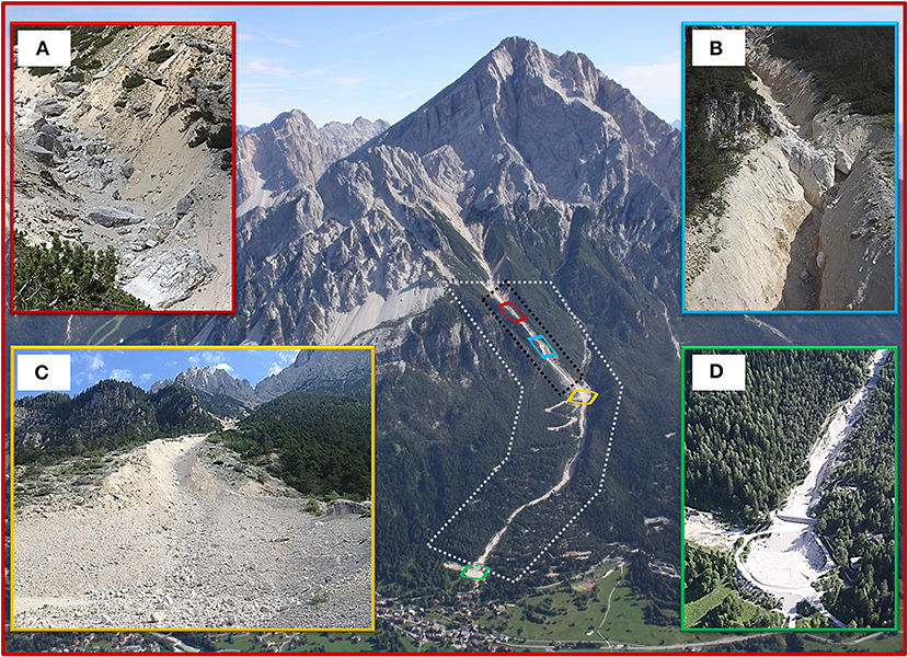
Figure 1. Aerial view of the Rovina di Cancia study site. (A) Debris flow triggering area (~1,670 m a.s.l.), (B) natural rock step located at the end of the debris flow triggering area (~1,500 m a.s.l.), (C) man-built flat deposition area (~1,340 m a.s.l.), (D) final flat circular deposition basin (~1,000 m a.s.l.). Dotted white line: LiDAR data coverage and hydraulic model domain; dotted black line: RTK-GPS data coverage.

From a geomorphological point of view, the debris flow catchment can be divided into three main sectors. In the upper part, massive rock cliffs prevail. They are composed of Upper Triassic to Lower Jurassic dolomites and limestones, underlined by the Raibl Formation, in a typical dolomitic stratigraphy configuration. The medium part is characterized by screes of poorly sorted and highly permeable debris, with boulders that can reach diameters of about 3–4 m, while the downstream part is covered by old debris flow deposits, including postglacial sediment material.

The Cancia area is prone to stony debris flows owing to the plenty availability of loose and coarse sediments, and the impulsive hydrological regime of the basin. In particular, the smaller grain sized material is provided by both the failure and the erosion of the banks, whereas gravel, pebbles and cobbles are provided by the upper part of the basin characterized by rocky material. The pluviometric regime of the area is characterized by short duration and high intensity rainfall events, usually occurring during the summer season (Gregoretti and Dalla Fontana, 2007).

Different stony debris flow events have been recorded in the past decades probably due to recent changes in the rainfall pattern. The most significant ones are those occurred on 2 July 1994, on 7 August 1996, and on 18 July 2009 (Simoni et al., 2018). The first flooded the inhabited fan with about 30,000 m³ of debris. The second mobilized about 45,000–60,000 m³ of debris damaging some houses and cars but without losses of human life, while the latter mobilized about 40,000 m³ of debris and, after the filling of the retaining basin, it flooded some houses causing two casualties. The most recent debris flow events are those occurred on 23 July 2015 (about 30,000 m³ of mobilized debris) and on 4 August 2015 (about 25,000 m³ of mobilized debris).

Data Acquisition

Full-waveform aerial laser scanner survey

The study site of Rovina di Cancia was surveyed by Helica s.r.l. on 21 October 2015 by using a I-HBEP helicopter (Eurocopter AS 350 B3) equipped with a long-range, small footprint, full-waveform RIEGL LMS-Q780™ sensor. A comprehensive overview on the Airborne Laser Scanning (ALS) can be found in Vosselman and Maas (2010), while the state-of-the-art on the full-waveform topographic LiDAR systems as well as on the related data processing techniques can be found in Mallet and Bretar (2009) and Wagner et al. (2006). The employed instrument works according to the time-of-flight distance measurement principle, and makes use of a powerful laser source, multiple-time-around processing, echo digitalization, and waveform analysis. This combination allows the operation at varying flying altitudes, and it is therefore ideally suited for aerial survey of wide areas and complex terrains. The ALS system was completed by five Global Positioning System (GPS) ground stations located within a maximum distance of 50 km from the surveyed area, which served as reference stations for the off-line differential GPS calculation. Furthermore, a Phaseone iXA 180 medium-format frame digital camera was accommodated on the scanner assembly ground plate, thus allowing the simultaneous acquisition of range and image data. The technical features of the employed laser-scan system as well as the employed flight parameters are reported in Tables 1S, 2S of the Supplementary Material, respectively.

After the aerial survey, the LiDAR data provider classified the raw points cloud into ground and non-ground echoes through the software package Terrascan™, setting parameters refined by the company itself over the years. For the study area of Rovina di Cancia (Figure 1), the mean LiDAR points density (i.e., ground and non-ground points density) was 20.79 points m⁻². After the filtering step, the mean LiDAR ground points density resulted in 3.33 points m⁻², corresponding to a mean ground points distance of 0.28 m.

Real-time kinematic gps survey

To assess the vertical accuracy of both LiDAR data and interpolated DEMs (see subsections LiDAR data pre-processing and vertical accuracy analysis, and DEMs generation and interpolation algorithms comparison), over 3,000 independent Real-Time Kinematic GPS (rtkGPS) measurements were acquired on October-November 2015 by using a dual frequency Topcon HiPer V GPS base and rover system (Figure 1 and Figure 1SA of the Supplementary Material). This ground-based survey technique ensures high-accuracy topographic measurements that can be regarded as control values for laser scanning- and photogrammetric-derived points clouds (Cilloccu et al., 2009; Caroti and Piemonte, 2010). As a matter of fact, the nominal positioning accuracy for dual-frequency GPS systems operating in kinematic mode and with baseline less than 20 km ranges between 0.02 and 0.05 m. Since the control values should be at least three times more accurate than data being evaluated (e.g., Höhle and Höhle, 2009; Höhle and Potuckova, 2011), it means that the rtkGPS measurements can be used to assess the accuracy of points clouds having positioning accuracy up to 0.06 m.

In order to describe the channel morphology as accurate as possible, a cross-sections morphological-guided spatial sampling scheme was adopted (e.g., Aguilar et al., 2005; Heritage et al., 2009). In detail, the ground measurements were acquired in coded cross-sections keeping orthogonal to the flow direction, and taking care to acquire relevant topographic features (e.g., talweg position, toe and top bank, Figure 1SB of the Supplementary Material). Both the ground points sampling distance and the cross-sections inter-distance were defined during the field survey according to the terrain roughness. The mean points sampling distance was 0.65 m (with a maximum of 2.73 m, and a minimum of 0.06 m), whereas the mean cross-sections inter-distance was 3.25 m (with a maximum of 9.80 m, and a minimum of 0.89 m).

The real-time three dimensional rover position was obtained by connecting via radio waves to a master station located at a maximum distance less than 1 km in order to minimize the measurement errors (Figure 1SA of the Supplementary Material). The positioning was based on phase solutions employing both L1 and L2 signal frequencies. To achieve the maximum accuracy, during the ground survey only fixed solutions were acquired. In addition, the three dimensional position of each surveyed ground point was calculated as the average of the measurements carried out on five epochs. This measurements redundancy allowed minimizing the influence of the inherent error sources (e.g., atmosphere delay, multipath, and clocks synchronization). The reported RTK-GPS data planimetric precision was 0.005 ± 0.001 m (with a maximum of 0.03 m), while the reported vertical precision was 0.008 ± 0.002 m (with a maximum of 0.05 m). The average planimetric dilution of precision value was 2.55 ± 0.45 (with a maximum of 3.50). The average number of GPS satellites viewed during the survey (GPS and GLONASS constellations) was 10 (with a maximum of 14).

The geographic coordinates of the rtkGPS measurements were projected in the coordinate system WGS84-UTM32 (i.e., the LiDAR data geodetic-cartographic datum, see subsection LiDAR data pre-processing and vertical accuracy analysis), whereas the orthometric heights were computed based on the local geoid model ITALGEO2005¹.

GIS-Based Routing Cell Model

The employed GIS-based debris flows cell routing model is able to simulate the routing and the entrainment-deposition processes of solid-liquid mixtures having a grain-collision dominated rheology (Gregoretti et al., 2018a), also known as stony debris flows (Takahashi, 2007). It represents the fully bi-phase version of the one proposed by Gregoretti et al. (2016a), and it allows a better simulation of the entrainment process.

The model discretizes the flow domain by using the square cells of a DEM. Each cell is hydraulically linked with its eight surrounding ones (Figure 2SA of the Supplementary Material), and the flow always occurs according to positive free surface drops (Figures 2SB,SC of the Supplementary Material). The governing equations of the mathematical model are those of mass and momentum conservation of both the overall sediment-water mixture and the solid phase, along with the Exner's equation in union with a modified version of the one dimensional empirical law of Egashira and Ashida (1987) for the rate of change of bed elevation.

In differential form, the continuity equations at the cell scale are:

$\begin{array}{cc}\begin{array}{r}A\frac{d(h+z)}{dt}+{\sum }_{k=1}^8{Q}_k=0\end{array}& (1)\end{array}$

$\begin{array}{cc}\begin{array}{r}A\frac{d(ch+c*z)}{dt}+{\sum }_{k=1}^{8}c{Q}_k=0\end{array}& (2)\end{array}$

where A is the area of the square cell, h is the flow depth, z is the bottom elevation, t is the time, c is the sediment volumetric concentration of the mixture, c${}_{{}^{*}}$ is the dry sediment concentration (also known as maximum packaging concentration), and Q_k is the discharge exchanged by the reference cell with its surrounding ones, assumed to be positive if outflowing and negative otherwise.

In the model, the water-sediment mixture is supposed to be a continuous mean composed by granular material immersed in an interstitial fluid, with equal velocities for the two phases according to Rosatti and Begnudelli (2013). Following the kinematic wave approximation as in Lenzi et al. (2003) and Di Cristo et al. (2014), in the case of gravity-driven flow (Figure 2SB of the Supplementary Material) the momentum equation is that of uniform flow in a Chezy-like form. Conversely, in the case of flow along negative slopes (Figure 2SC of the Supplementary Material) the momentum equation is that of broad-crested weir. This latter equation is used to cope with flow routing in areas having local topographic depressions, and in the presence of obstacles like hydraulic structures and houses. The two momentum equations are:

$\begin{array}{cc}\begin{array}{r}\begin{array}{cc}{Q}_k=Ch\Delta x{w}_k\sqrt{ghsin{\vartheta }_k}& w_k=\frac{sin{\vartheta }_k}{{\sum }_{k=1}^{n}sin{\vartheta }_k}\end{array}\end{array}& (3)\end{array}$

$\begin{array}{cc}\begin{array}{r}\begin{array}{cc}{Q}_k=0.385\Delta x{s}_k\sqrt{2g}{(h-z_k)}^{1.5}& s_k=\frac{h-z_k}{{\sum }_{k=1}^m(h-z_k)}\end{array}\end{array}& (4)\end{array}$

where C is the conductance coefficient (Tsubaki, 1972) representative of the grain-inertial rheology (Takahashi, 1978, 2007), Δx is the cell size, w_k and s_k are weighting functions introduced in order to allow multi-flow directions, g is the gravity acceleration, h is the flow depth, z is the bottom elevation, and ϑ_k is the angle formed with the horizontal by the line joining the center of the reference cell with its surrounding ones.

The Exner's equation is:

$\begin{array}{cc}\begin{array}{r}\frac{dz}{dt}=-i_b\end{array}& (5)\end{array}$

$\begin{array}{cc}\begin{array}{r}{i}_b=K{U}_{MAX}(sin{\alpha }_{MAX}-sin{\vartheta }_{LIM})\end{array}& (6)\end{array}$

where i_b is the rate of change of bed elevation as proposed in Gregoretti et al. (2016a), K is an empirical constant ranging between 0 and 1, U_MAX is the velocity corresponding to the steepest of the eight possible flow directions k_MAX, α_MAX is equal to ϑk_MAX in the case of gravity-driven flow, otherwise α_MAX is equal to (ϑ_K + Θ_k)_MAX being Θ_k the angle that the horizontal forms with the line joining the flow surface of the reference cell with that of the cell where the flow is directed, ϑ_LIM and U_LIM are limit values for ϑ and U, respectively. The parameters ϑ_LIM and U_LIM assume different values for erosion (U_LIM-E and ϑ_LIM-E) and deposition (U_LIM-D and ϑ_LIM-D), and they should be determined by field measurements or numerical back-analysis. The erosion velocity i_b is positive if U_MAX > U_LIM-E and α_MAX > ϑ_LIM-E, whereas it is negative if U_MAX < U_LIM-D and α_MAX < ϑ_LIM-D. Erosion and deposition are computed only along the steepest downslope flow direction because considering all the possible flow directions could lead to unrealistically large deposition rate along directions transverse to the steepest downslope flow direction, and a cell could be subjected to both erosion and deposition in the same time interval. Erosion is only computed for increasing flow depths (dh/dt > 0), according to the instrumental field observations of Berger et al. (2011). Other two constrains are imposed to erosion and deposition processes: entrainment of sediment by the overflowing mixture is possible only if c is smaller than the physic limiting upper value of 0.9c${}_{{}^{*}}$ (Takahashi, 2007); similarly, deposition occurs only if c is larger than a limiting lower sediment concentration for debris flow (c_D) assumed equal to 0.05.

From a numerical point of view, the governing equations are solved by using the finite difference technique with an explicit scheme subject to the Courant-Friedrichs-Lewy stability condition. The initial conditions are represented by the inflow solid-liquid hydrograph computed by means of a triggering model (e.g., Gregoretti et al., 2016b, 2018a,b). The computation procedure starts defining for each cell the possible solid-liquid discharges toward its eight surrounding ones according to Equations (3, 4). Then, the rate of change of bed elevation corresponding to the steepest downslope flow direction is computed by Equation (6). At the end of each computational time step, the cell free surface and bed elevation are simultaneously updated based on the computed outflow/inflow and deposited/entrained volumes.

LiDAR Data Pre-Processing and Vertical Accuracy Analysis

Raw and filtered LiDAR datasets were delivered in ASCII files consisting of X, Y, Z coordinates (ellipsoidal heights related to the reference ellipsoid WGS84) and intensity data, arranged in 1 × 1 km tiles based on the projected coordinate system WGS84-UTM32. Although at national and regional level the geodetic-cartographic datum Roma40-Gauss Boaga represents the formally accepted coordinate system, no datum transformation was performed in order to avoid accuracy loss in the delivered topographic datasets. Conversely, the ellipsoidal heights were converted in orthometric heights based on the local geoid model ITALGEO2005, thus allowing the direct comparison with the GPS validation measurements (see subsection Real-time kinematic GPS survey). No additional attributes (e.g., GPS time for every laser shot, scan angle, edge of flight line information, echo amplitude, echo width) were included within the delivered datasets.

Before analysing the vertical accuracy of the aerial laser data, the filtered LiDAR dataset was converted in LAS format and then critically examined to check for classification errors (i.e., commission and omission errors). It represents a key step since the LiDAR-derived DEMs quality strongly depends on the correct classification of the raw points cloud into terrain and off-terrain echoes (e.g., Vosselman and Maas, 2010). The visual inspection of the LiDAR data via LASview™² highlighted many data voids in morphologically complex areas, mainly due to misclassified LiDAR points as non-ground when they truly represented ground features such as big boulders within the channel (Figure 3S of the Supplementary Material). As this kind of classification errors could heavily affect the routing model outcomes, the delivered raw points cloud was re-classified into ground and non-ground points within the software package LAStools™. For the study area of Rovina di Cancia, the re-classification procedure yielded a mean LiDAR ground points density equal to 4.34 points m⁻² (i.e., 30% more than the density of the delivered LiDAR ground points dataset), with an observed mean ground points distance corresponding to 0.25 m.

Since a number of error sources can affect the accuracy of LiDAR points clouds determining systematic errors and many outliers (e.g., accuracy in the aircraft absolute positioning and attitude data, accuracy of system calibration as determination of boresight angles and offsets between instruments, internal scanner errors, automated processing of the points cloud), an extensive vertical accuracy assessment was carried out on the re-classified LiDAR ground points dataset by using the independent rtkGPS measurements. An automated routine based on a proximal point algorithm (e.g., Reutebuch et al., 2003; Webster and Dias, 2006; Pourali et al., 2014) was then coded in order to directly compare the LiDAR and the validation data. This approach is suitable to accurate heights comparison since the errors introduced through the data gridding are eliminated (Hodgson and Bresnahan, 2004; Höhle and Potuckova, 2011; Pourali et al., 2014). The validation technique involves a user specified horizontal search radius around the GPS control point for comparison with the LiDAR ground points. In order to limit the influence of channel slope on the computed elevation residuals, a horizontal search radius equal to 0.50 m was used. It has also allowed an average number of LiDAR ground points within the search radii equal to four, thus ensuring a sufficient sample size for reliable accuracy measures. All LiDAR ground points within that search area are selected, and then their orthometric heights are compared to that of the GPS validation point. The computed elevation differences were regarded as vertical “errors,” and they were statistically analyzed within the R open-source software package (R Development Core Team, 2008).

The derivation of accuracy measures has to take into account that outliers may exist, and that the distribution of the errors might not be normal. For this reason, the framework outlined in Höhle and Potuckova (2011), based on the standard (e.g., mean error, standard deviation, and their confidence intervals) and robust accuracy measures (e.g., median, Normalized Median of Absolute Deviations (NMAD), sample quantiles of absolute errors, and their confidence intervals) reported in Table 3S of the Supplementary Material, was followed. The reader is referred to the works of Höhle and Höhle (2009) and Höhle and Potuckova (2011) for a complete dissertation of the method.

It is worth pointing out that we compared two points datasets having different measurement support size, location, and spatial distribution, which poses inherent uncertainties on the accuracy assessment results.

DEMs Generation and Interpolation Algorithms Comparison

DEMs Interpolation

Prior to DEMs interpolation, a thoroughly Exploratory Spatial Data Analysis (ESDA) was performed on the re-classified LiDAR ground points dataset. This analysis was carried out at the purpose of gaining insight into the studied spatial variable. A number of features of the topographic dataset were investigated by the ESDA tools of the Geostatistical Analyst™ module (ArcGIS™, rel. 10.3), among which: spatial and marginal distribution via Voronoi's polygon map, points pattern analysis, and standard statistic plots and indices; second-order or intrinsic stationarity by trend analysis; and spatial dependency through variography.

Among the tested interpolation methods, the TIN-based routines (i.e., linear triangulation, natural neighbor, and nearest neighbor) does not require a dataset specific parametrization. Conversely, the remaining deterministic (i.e., Inverse Distance to a Power, ANUDEM, and Radial Basis Functions) and geostatistical (i.e., point ordinary kriging, and block ordinary kriging) methods were parameterized as it follows.

The most important parameters of IDP and RBFs algorithms were optimized via cross-validation, by minimizing the mean square prediction error. As a matter o fact, in its common form of “leave one out” it represents the most frequently used exploratory mean to find the best dataset specific algorithm parametrization (Erdogan, 2009). According to Oliver and Webster (2014), these algorithms were also parametrized to use during the interpolation procedure a number of neighbors ranging from 7 to 25. Furthermore, the presence of a linear global trend following the channel gradient (see subsection Exploratory spatial data analysis results and Figure 4A) led to the use of a one sector elliptical search neighborhood, oriented according to the direction of the greatest spatial continuity (i.e., the direction perpendicular to the trend). The ellipse major semi-axis was set equal to the range of the directional empirical variogram computed along the direction of the greatest spatial continuity. Conversely, the ellipse minor semi-axis, corresponding to the direction of the least spatial continuity (i.e., the trend direction), was defined by cross-validation. This search strategy allowed to favor during the interpolation procedure the points with the greatest spatial correlation. The ANUDEM algorithm was tested using only the re-classified LiDAR ground points as input data. The algorithm roughness penalty was defined as a mixture of minimum curvature and minimum potential, and the drainage enforcement option was enabled. Moreover, the standard vertical error and the first elevation tolerance were set equal to the computed random vertical error of the re-classified LiDAR points dataset (see subsection LiDAR data vertical accuracy assessment and Table 1). The geostatistical interpolation was performed through the ordinary kriging algorithm, employing a Gaussian theoretical variogram model fitted on the directional empirical one computed perpendicularly to the trend. In fact, as suggest by Chiles (1984) and Oliver and Webster (2014), a statistically sound procedure to kridge points dataset with a dominant linear global trend consists in applying the ordinary kriging algorithm using a theoretical variogram model fitted on the directional empirical one computed along the direction of the greatest spatial continuity. This theoretical variogram can be regarded as the variogram of the residuals (i.e., the theoretical variogram of the spatially correlated component of the studied variable). The nugget parameter of the theoretical variogram was set equal to the square of the computed random vertical error of the re-classified LiDAR points dataset, so predicting filtered (or, “error-free”) values. Furthermore, the points dataset was kridged using both a punctual and a block support, with a block dimension corresponding to 0.50 and 1.00 m (i.e., the DEMs spatial resolution, see below). For the upscaling procedure, the number of averaged punctual predictions within each block was defined according to the LiDAR footprint, which represents the input data support dimension. All the employed interpolation techniques parametrizations are summarized in Table 4S of the Supplementary Material.

TABLE 1

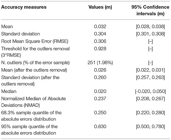
Table 1. Computed standard and robust accuracy measures.

The spatial resolution of DEMs was set according to the rules outlined by Hengl (2006). In detail, the author proposed empirical and analytical criteria to select the optimal grid resolution for points dataset interpolation, including those based on GPS horizontal error, map scale, size and shape of the smallest objects being mapped, points pattern geometry, and spatial correlation. Many of the described methods refer to the Whittaker-Nyquist-Kotelnikov-Shannon sampling theorem (e.g., El-Sheimy et al., 2005), which states that an original continuous signal can be reconstructed from the sampled data (without any loss of information) only if the sampling frequency is twice than the original one (Nyquist frequency). Thus, a raster grid cell size that retains the highest information content of the original points dataset is equal to half the average spacing between the closest points pairs. The re-classified ground LiDAR points were randomly distributed with an average mutual distance equal to 0.29 m. However, the 5% quantile of the nearest neighbor distances distribution was 0.10 m, while the 95% quantile was 0.57 m (Table 5S of the Supplementary Material). Therefore, a spatial resolution of 0.05–0.30 m was deemed to be appropriate for the employed LiDAR dataset. Nevertheless, the processing power of the available hardware along with the data management efficiency of GIS software limit the ability to generate digital surfaces at these very fine spatial resolutions. Thus, for each combination of interpolator and related parameters, DEMs were generated with a spatial resolution equal to 0.50 and 1.00 m (corresponding to 2.17 and 4.34 ground LiDAR points per cell, respectively). Notably, a spatial resolution of 0.50 m matches the source data information content according to the root mean square slope criterion developed by Hutchinson (1996).

Comparison of Interpolation Methods

Once the DEMs were generated, the overall performance of each tested interpolation algorithm was assessed by computing the vertical bias and accuracy of the corresponding gridded digital surface through the independent rtkGPS points dataset. In detail, the accuracy measures were statistically derived starting from the differences between the rtkGPS height value and the elevation value of the grid cell center containing the rtkGPS point itself. In order to choose between standard or robust accuracy measures (see subsection LiDAR data pre-processing and vertical accuracy analysis and Table 3S of the Supplementary Material), the sample error distributions were firstly check for outliers and normality. The outliers threshold was set equal to three times the Root Mean Square Error (RMSE) according to the rules outlined by Höhle and Höhle (2009), whereas the sample error distributions normality was tested both graphically by means of the normal Q-Q plot, both statistically through the D'Agostino K² omnibus test. This statistical test was choosen for its reliability with large data samples having kurtosis slightly higher than the normal distribution (Gallay et al., 2013). Therefore, the median of the vertical errors was chosen as robust estimator of the DEMs vertical bias, whereas, for the vertical accuracy of DEMs, the NMAD along with the 68.3 and 95% quantiles of the absolute errors distribution were chosen as robust estimators. The Mean Absolute Error (MAE), the minimum and maximum vertical error and the corresponding range, the weighted determination coefficient (Krause et al., 2005) along with the slope and the intercept parameters of the linear regression between measured and interpolated values, and the total drainage sink area (i.e., number and extension of raster cells whose neighbors are all of higher elevation) were also used as supplementary DEM quality indices. This latter index was used here as interpolation errors indicator, since the higher the number of interpolation artifacts in the gridded DEM, the larger the total drainage sink area will be (Wise, 2000, 2007; Setiawan et al., 2013).

It is worth pointing out that all these descriptive statistics are aspatial (i.e., spatially uniform) summary accuracy indices. However, a number of authors suggested that the vertical error of DEMs is not spatially uniform, but it can assume some form of spatial pattern (e.g., Li, 1993; Wood and Fisher, 1993; Wood, 1996; Yang and Hodler, 2000; Weng, 2006; Erdogan, 2009). Since DEMs with identical global accuracy values may have a different spatial pattern of errors (with digital surfaces having evenly distributed error values more reliable than those with high error clustering), to evaluate the performance of an interpolation method it is also important to investigate the spatial distribution of the vertical errors and their clustering extension. For deterministic gridding methods, the best way to examine the spatial distribution of the vertical errors is by means of accuracy maps obtained after comparing the interpolated DEM with a second more accurate surface. These maps have the advantage of clearly indicate where serious and perhaps anomalous errors occur. Unfortunately, as in this study, the availability of a more accurate control surface for comparison is rare. Thus, the spatial distribution of the vertical errors was graphically investigated through choropleth symbol maps, in which the size and the color of each independent validation point is established according to the error magnitude. Conversely, the error clustering extent was statistically assessed by means of both global and local indicators of spatial autocorrelation (i.e., the Global Moran's I index and the Anselin Local Moran's I index, respectively). The Global Moran's I index measures the overall spatial autocorrelation based on both features location and features value simultaneously, so evaluating whether the pattern expressed is clustered (index value approaching to 1), dispersed (index value approaching to −1), or random (index value approaching to 0). Noteworthy, it indicates clustering of high or low error values, but without showing where the clusters are. To overcome this drawback, the Anselin Local Moran's I index was also used in the error clustering assessment. As the name suggests, it represents the local form of the Global Moran's I index, and it is used to graphically detect local pockets of dependence.

Since a critical concern in assessing the reliability of a gridding method is represented by its sensitivity with respect to changes in certain parameters (e.g., search neighborhood) or conditions (e.g., sample size; Yang and Hodler, 2000), we further evaluated the stability (or robustness) of each tested interpolation algorithm focusing on the sample size. In detail, we investigated the change in the performance of each tested gridding method considering a decreasing number of LiDAR ground points. Therefore, thinned datasets were obtained by randomly splitting the re-classified LiDAR ground points at densities equal to 95%, 75%, and 50% (which correspond to 4.13, 3.29, and 2.64 points m⁻², respectively). These thinned sample datasets were therefore interpolated at the spatial resolution of 0.50 and 1.00 m, keeping unchanged for each gridding technique the optimized model parameters (Table 4S of the Supplementary Material). After that, on each thinning-derived DEM, a comprehensive accuracy assessment was carried out following the approach above outlined, and the results obtained at the vary sample densities were finally compared. Note that a total of 96 DEMs were generated for this investigation.

As recognized by vary authors the success of a digital terrain modeling algorithm mainly depends on the purposes (e.g., Hengl and Reuter, 2009; Schwendel et al., 2012). Unlike DEMs for ortho-photos production where the absolute accuracy of the elevation values is the most important feature, DEMs for hydrological and hydraulic modeling must represent the catchment and channel shape realistically and close to the sampled topographic data. It ensures that slopes and flow paths are correctly represented in the interpolated DEM. For this reason, the shape reliability of each generated DEM was investigated by combining visualization techniques and residual analysis. The shape reliability is here defined as the degree of maintenance of the channel shape (as described by the sampled topographic data) in the interpolated DEM. In a pre-selection phase, for each generated DEM derivatives like slope, aspect, and curvature, along with shaded relief and surface roughness maps, were visually examined in order to identify interpolation artifacts. For the gridded surfaces that ensured a satisfactory representation of the channel topography, a multi-criteria morphological based comparison was then undertaken. The established morphological criteria include the plano-altimetric representation of longitudinal and transversal linear features (e.g., channel margins, hydraulic structures, and steps), and the representation of channel bottom forms (e.g., sediment sheets, boulders, and rugged reaches). They were defined considering the morphological features of the channel that need to be correctly maintained in the interpolated DEM in order to guarantee a reliable numerical modeling of debris flows routing. Noteworthy, this approach relies on qualitative analysis depending on the expert judgment of a user, and it represents its main limit. Therefore, in order to overcome this drawback, the ability of each tested gridding method to fulfill the topographic sampled data (i.e., the ability to faithfully represent the surveyed topography) was quantitatively assessed through a residual analysis.

Evaluation of the Effects of the Gridding Techniques on Debris Flow Routing Model Results

The hydraulic simulation of the Rovina di Cancia debris flow was carried out by using the cell routing model proposed by Gregoretti et al. (2018a) and described in subsection GIS-based routing cell model.

Since the effects of the digital elevation uncertainty resulting from the gridding procedure on debris flows routing modeling could be masked by an inaccurate model parametrization, the input parameters of the cell model were previously calibrated against two real debris flow events (occurred at Rovina di Cancia on 18 July 2009 and on Ru Secco the 4th of August 2015, respectively). In detail, the calibration procedure was undertaken by comparing the simulation results with both the observed erosion/deposition depth maps and the witnessed routing times. Both the back-analysis provided the same optimal model parametrization, thus guaranteeing a certain high degree of predictivity (for further details see Gregoretti et al., 2018a,b).

For all the model runs, both the calibrated values of the input parameters (i.e., C, K, U_LIM-D, U_LIM-E, ϑ_LIM-D, and ϑ_LIM-E) and the initial conditions (i.e., the upstream solid-liquid hydrograph) were kept unchanged, varying only the initial topographic surface generated according to the twelve tested interpolation algorithms. Therefore, this approach allowed the investigation of the influence of the algorithms itself on modeling outcomes.

Two event scenarios, corresponding respectively to 50- and 300-years return period, were defined by means of a coupled hydrological and triggering model (e.g., Gregoretti et al., 2016b, 2018a,b), starting from the rainfall depth-duration frequencies curves. It enabled to investigate the influence of the gridding methods on debris flows routing model results for events having different magnitude, characteristics of two usual design return periods.

For the sake of simplicity, in the different model runs we employed only the full dataset- and the 50% thinning-derived 1-meter resolution DEMs as input topographic data, carrying out a total of 48 simulations (i.e., twelve DEMs, two points densities, and two event scenarios).

To evaluate the influence of the gridding methods on debris flows routing modeling, we initially explored the relationship between the uncertainties on digital elevation and on the model results. In detail, for each combination of points density and event scenario we correlated the pixel-wise standard deviation of the twelve DEMs heights (i.e., the standard deviation at the cell scale of the elevation values of the twelve input topographic data of the routing model) and the pixel-wise standard deviation of the corresponding twelve simulated erosion/deposition depths (i.e., the standard deviation at the cell scale of the corresponding twelve routing model outputs). This allowed elucidating if the cells with high uncertainty in the simulated erosion/deposition depths were spatially linked to those with high topographic uncertainty. It must be noted that the correlation was investigated both globally (i.e., at the channel extent) and locally by means of moving windows. The moving window size was set equal to 3 × 3 and 5 × 5 m, according to the spatial continuity of the correlated variables. The bivariate moving windows correlation analysis was carried out through the R package developed by Evans (2017). After that, for each combination of data density and event scenario, we compared the model run results in terms of simulated areas, erosion and deposition volumes, solid-liquid discharges, and channel morphology after the event.

Results and Discussion

LiDAR Data Vertical Accuracy Assessment

The results of the vertical accuracy assessment carried out on the re-classified LiDAR points cloud are summarized in Table 1. It turns out that the outliers have a great influence on the mean and standard deviation of the vertical errors values. Respectively, they drop from 0.032 to 0.026 m and from 0.304 to 0.260 m after the outliers removal. The histogram and the normal Q-Q plot shown respectively in Figures 2A,B highlight that the vertical errors distribution is non-normal. In particular, the histogram shows that the kurtosis of the vertical errors distribution is positive (i.e., the distribution has a more acute peak around the mean and fatter tails than the normal one). Furthermore, the normal Q-Q plot deviates from the straight line at the extremes, which clearly indicates the presence of outliers in the vertical errors sample. After the outliers removal, the values of the mean and standard deviation of the vertical errors decrease (Table 1), remaining any way somewhat greater than the corresponding robust ones (i.e., greater than the values of the median and NMAD of the vertical errors; see subsection LiDAR data pre-processing and vertical accuracy analysis and Table 3S of the Supplementary Material). Furthermore, the histogram and the normal Q-Q plot shown respectively in Figures 2C,D highlight that the thresholded vertical errors distribution does not follow the normal one.

FIGURE 2

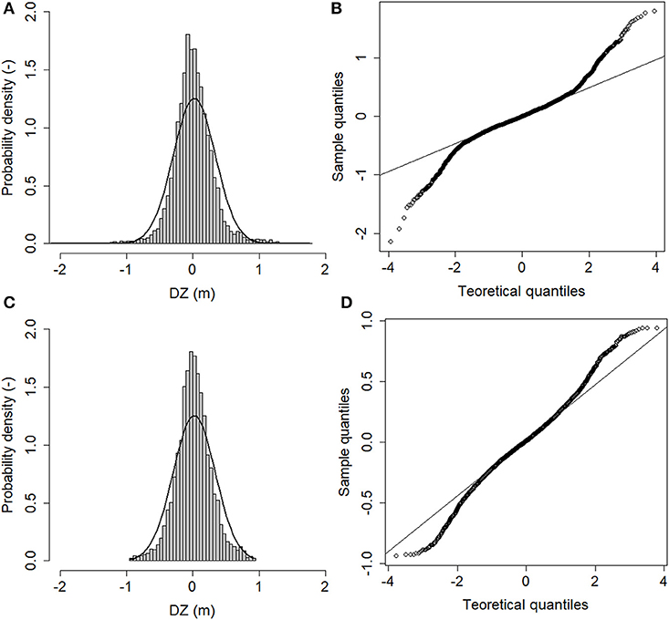
Figure 2. (A) Histogram of the errors dataset. Superimposed, the normal distribution with mean and standard deviation estimated from the original errors dataset. (B) Normal Q-Q plot of the errors dataset. (C) Histogram of the errors dataset without outliers. Superimposed, the normal distribution with mean and standard deviation estimated from the thresholded errors dataset. (D) Normal Q-Q plot of the errors dataset without outliers. DZ denotes the vertical error.

The median of the vertical errors is 0.020 m, and it represents the systematic vertical shift between the re-classified LiDAR points cloud and the rtkGPS validation data. This altimetric bias has been eliminated by means of a 2.5D calibration procedure (i.e., a rigid translation in the Z dimension of the re-classified LiDAR points cloud). After the calibration procedure, the vertical accuracy of the re-classified LiDAR points cloud only depends on its random vertical error component, and it can be evaluated by means of the standard deviation of the vertical errors. In this case, the robust estimator of the standard deviation is equal to 0.237 m, and it corresponds approximately to the 68.3% quantile of the absolute vertical errors distribution.

Figure 4S of the Supplementary Material depicts the difference between the employed accuracy measures. It has been obtained by superimposing to the vertical errors sample distribution the normal ones calculated by using the mean and the standard deviation of the vertical errors sample, the mean and the standard deviation of the vertical errors sample without outliers, and the median and the NMAD of the vertical errors sample, respectively. On one hand, the graph shows that the standard accuracy measures are not able to match the vertical errors sample distribution. Furthermore, even the application of an outliers threshold does not eliminate each of them from the vertical errors sample, and so the standard accuracy measures remain inaccurate. On the other hand, since the robust accuracy measures are able to apply a smoother transition between accepting or rejecting an observation from the vertical errors sample, they fit the vertical errors sample distribution best, both near the mean and at the tails. This finding validates the suggestions proposed by Höhle and Höhle (2009), who recommend the use of robust accuracy measures (i.e., median, NMAD, and sample quantiles of the absolute errors distribution) when the histogram (or the normal Q-Q plot) of the errors sample distribution reveals non-normality, since they are not influenced by the outliers or by the distribution skewness.

Exploratory Spatial Data Analysis Results

The results of the spatial distribution analysis carried out on the re-classified LiDAR points dataset are summarized in Table 5S of the Supplementary Material. The mean Voronoi's influence area of the LiDAR ground points is equal to 0.237 m², with an interquartile range corresponding to 0.174 m². It means that the spread of the influence area values is small, and so the sampling network can be considered homogeneous. Moreover, the average mutual distance between closest LiDAR points pairs is equal to 0.29 m ± 0.13 m, with a maximum of 3.48 m. The 5% quantile of the mutual distances distribution corresponds to 0.10 m, while the 95% quantile is equal to 0.57 m. The former statistic can be regarded as a robust measure of the minimum distance between closest ground points pairs, whereas the latter as a robust measure of their maximum distance.

As shown in Figure 3A, the marginal distribution of the re-classified LiDAR dataset is roughly unimodal, approximatively symmetric (skewness coefficient equal to 0.30), and approximatively mesokurtic (kurtosis equal to 2.40). However, the normal Q-Q plot deviates from the straight line at the extremes (Figure 3B), thus indicating that the elevation values distribution is non-normal. Moreover, the box-plot shown in Figure 3C does not reveal the presence of outliers within the dataset, as also confirmed by a coefficient of variation value lesser than one.

FIGURE 3

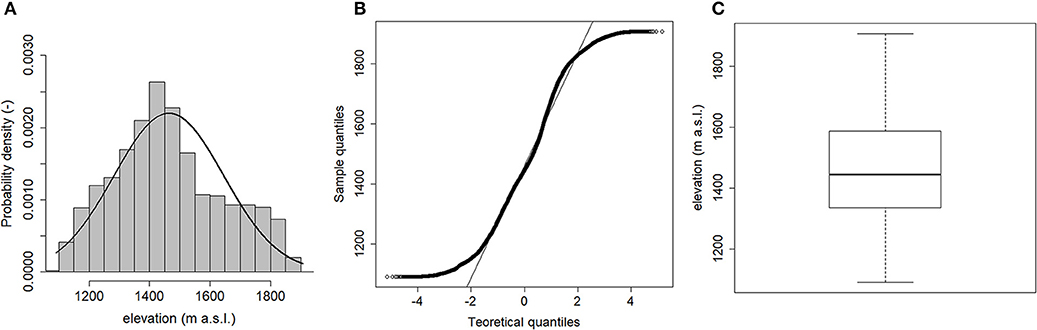
Figure 3. Histogram with superimposed the normal distribution (A), normal Q-Q plot (B), and box-plot (C) of the LiDAR ground points dataset.

The quantiles map of the elevation values (Figure 4A) clearly shows a trend in the NE-SW direction. It means that the variable to be interpolated is not stationary within the domain since its mean changes smoothly in the space. To find the trend degree, the correlation between the elevation values and the east-north spatial coordinates has been analyzed through the scatter-plots shown respectively in Figures 4B,C. The Pearson's correlation coefficient (referred as “rho Pearson”), which provides a measure of the linear relationship between two variables, is equal to 0.48 and 0.82 along the east and north direction, respectively. Often, it is useful to supplement the linear correlation coefficient with the Spearman's rank correlation coefficient (referred as “rho Spearman”), which represents a further measure of the relationship strength (Isaaks and Srivastava, 1989). Unlike the Pearson's coefficient, the Spearman's rank coefficient is not strongly influenced by extreme pairs, and large differences between the two correlation coefficients values may be due to the presence of few erratic pairs or to a non-linear relationship between the two variables. For the study area, the Spearman's rank coefficient is equal to 0.47 and 0.84 along the east and north direction, respectively. Since both along the east and north direction the differences between the Pearson's and Spearman's correlation coefficients values are small, it can be stated that the variable to be interpolated exhibits a linear global trend.

FIGURE 4

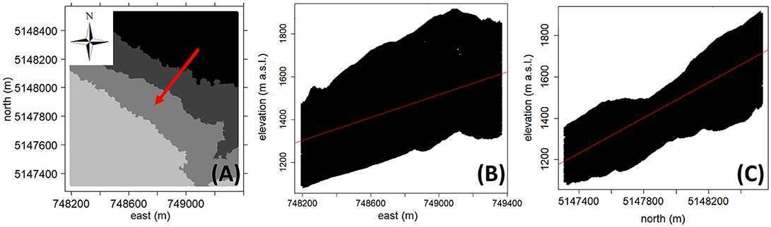
Figure 4. Quantiles map of the variable elevation (the red arrow indicates the trend direction, which corresponds to the channel gradient) (A), scatterplot elevation values versus east coordinate (rho Pearson = 0.48; rho Spearman = 0.47) (B), and scatterplot elevation values versus north coordinate (rho Pearson = 0.82; rho Spearman = 0.84) (C).

The directional empirical variogram of the elevation values computed perpendicularly to the channel gradient (i.e., along the direction of the greatest spatial continuity) is shown in Figure 5SA of the Supplementary Material, with overlying the fitted Gaussian theoretical variogram model. The theoretical variogram levels off at a range of about 180 m, reaching a plateau of 450 m². Furthermore, it exhibits a parabolic structure near the origin (Figure 5SB of the Supplementary Material), followed by an inflection point. The nugget to sill ratio along the considered variogram modeling direction is close to zero, thus indicating the presence of a strong spatial structure.

Comparison of Interpolation Methods

The computed global accuracy measures for each interpolated DEM are summarized in Table 2. For both the chosen spatial resolutions, all the tested interpolation algorithms provide a comparable small number of outliers (corresponding at about 1% of the vertical errors sample), however affecting the standard accuracy measures. Moreover, all the vertical errors sample distributions are non-normal (the only exception is the ANUDEM algorithm that yields a K² omnibus test p-value equal to 0.10 at the spatial resolution of 1.00 m). Overall, the median of the vertical errors is centimetric (smaller than ± 0.040 m), meaning that the interpolation bias can be regarded as negligible. However, a closer look of the computed median values reveals that only the ordinary kriging algorithm provides positive values (0.018 and 0.034 m at the spatial resolutions of 1.00 and 0.50 m, respectively). Furthermore, the ANUDEM and nearest neighbor algorithms yield the lowest median values at both the chosen spatial resolutions (respectively, −0.007 and −0.016 m at the spatial resolution of 1.00 m, and −0.016 and −0.006 m at the spatial resolution of 0.50 m), whereas the highest values are provided by the thin-plate spline plus tension (−0.031 m at the spatial resolution of 1.00 m) and ordinary kriging (0.034 m at the spatial resolution of 0.50 m) algorithms. The NMAD values range from 0.288 to 0.429 m, and from 0.201 to 0.337 m at the spatial resolutions of 1.00 and 0.50 m, respectively. At both the grid cell sizes, the thin-plate spline and multi-quadratic basis functions yield the lowest values (respectively, 0.288 and 0.288 m at the spatial resolution of 1.00 m, and 0.201 and 0.203 m at the spatial resolution of 0.50 m), whereas the ANUDEM and ordinary kriging algorithms show the lowest performance (i.e., the highest NMAD values, equal to 0.429 and 0.390 m at the spatial resolution of 1.00 m, and 0.347 and 0.337 m at the spatial resolution of 0.50 m, respectively). It must be noted that for all the tested gridding methods, the higher the spatial resolution of the interpolated DEM (i.e., the smaller the raster grid cell size), the smaller the corresponding NMAD value (i.e., the better the interpolation). This finding is in general agreement with that observed for example by Bater and Coops (2009), who noticed an improvement on the interpolation algorithms performance as the spatial resolution of the generated DEMs increased from 1.50 to 0.50 m. However, the percentages of NMAD variation (i.e., how much an interpolator increases its prediction accuracy as the spatial resolution increases) change according to the considered gridding algorithm. In detail, the thin-plate spline and multi-quadratic basis functions exhibit the greatest percentages of NMAD variation (corresponding to 29.90 and 29.38%, respectively), where the ordinary kriging algorithm along with the inverse multi-quadratic basis function show the smallest ones (corresponding to 13.69 and 15.72%, respectively). It means that although all the tested interpolation algorithms improve their performance as the chosen raster grid cell size decreases, for some of them the choice of an optimal spatial resolution is a more critical concern. The 95% sample quantiles of the absolute vertical errors distributions range from 0.770 to 0.945 m, and from 0.738 to 0.945 m at the spatial resolutions of 1.00 and 0.50 m, respectively. This statistic can be regarded as a robust measure of the maximum (unsigned) interpolation vertical error. For both the chosen spatial resolutions, the thin-plate spline and multi-quadratic basis functions yield the lowest quantiles values (respectively, 0.770 and 0.778 m at the spatial resolution of 1.00 m, and 0.745 and 0.738 m at the spatial resolution of 0.50 m), along with the linear triangulation (0.777 m) and the natural neighbor algorithm (0.777 m) only at the spatial resolution of 1.00 m. Conversely, the ANUDEM and ordinary kriging algorithms perform worst (i.e., yield the highest sample quantile values, equal to 0.922 and 0.945 m at the spatial resolution of 1.00 m, and 0.802 and 0.945 m at the spatial resolution of 0.50 m, respectively), along with the inverse multi-quadratic basis function (0.825 m) only at the spatial resolution of 0.50 m. It is worth pointing out that overall no significant differences in the computed accuracy measures are found among point and block ordinary kriging.

TABLE 2

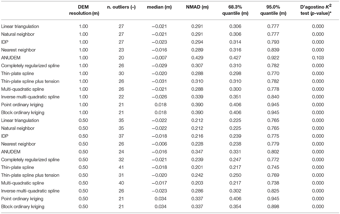
Table 2. Global accuracy measures for each interpolated DEM (* the values refer to the errors distribution after the outliers removal).

The supplementary DEMs quality measures along with the Global Moran's I index values are reported in Table 3. The MAE values range from 0.243 to 0.338 m, and from 0.184 to 0.329 m at the spatial resolutions of 1.00 and 0.50 m, respectively. At both the grid cell sizes, the thin-plate spline and multi-quadratic basis functions yield the lowest MAE values (respectively, 0.243 and 0.248 m at the spatial resolution of 1.00 m, and 0.184 and 0.187 m at the spatial resolution of 0.50 m), whereas the ANUDEM and ordinary kriging algorithms show the lowest performance (i.e., the highest MAE values, corresponding to 0.338 and 0.329 m at the spatial resolution of 1.00 m, and 0.266 and 0.329 m at the spatial resolution of 0.50 m, respectively). The vertical error range is between 2.212 and 2.812 m, and between 1.327 and 2.597 m at the spatial resolutions of 1.00 and 0.50 m respectively. The lowest error ranges are provided by the thin-plate spline (2.212 and 1.907 m, at the spatial resolutions of 1.00 and 0.50 m, respectively). Conversely, the ANUDEM and ordinary kriging algorithms return the highest error range values at the spatial resolution of 1.00 m (respectively, 2.711 and 2.812 m), whereas the ordinary block kriging performs worst at the spatial resolution of 0.50 m (2.597 m). Respect to the linear regression parameters, the intercept values are all negative at both the chosen spatial resolutions, with the worst results provided by the ANUDEM and ordinary kriging algorithms (approximatively −2.00 m). On the other hand, both the slope and the weighted regression coefficient values does not reveal noteworthy differences among the tested gridding methods, with all of them equal to one. The analysis of the total drainage sink area points out a correspondence between the spatial resolution increment and the number of pits, irrespective to the gridding algorithm. The only exception is the ANUDEM algorithm, which also provides (as expected) the lowest number of sinks at both the chosen spatial resolutions (respectively, 3 and 2). Conversely, the multi-quadratic basis function performs worst (i.e., it yields the highest number of sinks) at both the grid cell sizes (respectively, 30 and 273). It must be noted that the increase in the total drainage sink area is not only related to the cell size halving, but also to an increment in the number of pits. In other words, the higher the spatial resolution, the higher the number of interpolation artifacts. This finding is clearly in contrast with the previous one. However, it should be noted that the vertical accuracy assessment carried out on the interpolated DEMs has been performed by comparing two points datasets (i.e., the rtkGPS points and the grid cells centers containing the rtkGPS points themselves) that do not spatially overlap. Therefore, the better accuracy (i.e., the smaller NMAD values) of the finer gridded surfaces might be only due to the lower distances between the grid cell center and the rtkGPS validation point.

TABLE 3

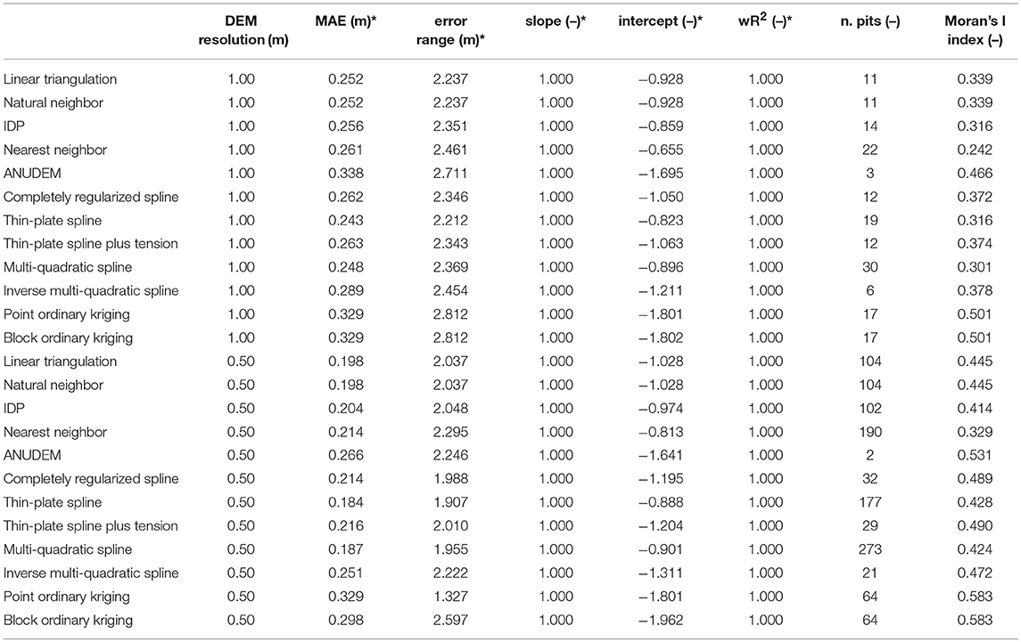
Table 3. Supplementary DEM quality indices and global Moran'I index values for each tested interpolation algorithm and chosen spatial resolution (* the values refer to the errors distribution after the outliers removal).

The analysis of the absolute errors spatial pattern by means of the visual inspection of choropleth symbol maps (Figure 5) reveals that for all the tested interpolation algorithms the greatest (unsigned) vertical errors occur in correspondence of breaks of slope (e.g., at the top of the banks) and in morphologically complex areas (e.g., in the upper part of the channel due to the presence of big boulders, and at the rock step located about 200 m downstream the initiation area (~1,500 m a.s.l.), Figure 1B), regardless of both the points density of the dataset used during the interpolation procedure and the chosen raster grid cell size. Moreover, within the channel there are subtle differences among the tested interpolation algorithms, and the spatial pattern of the vertical errors visually appears to be random. However, a closer look of these maps highlights some local pockets of spatial dependence common to all the tested methods, as also confirmed by the Anselin local Moran's I index maps (Figure 6). The Global Moran's I index values range from 0.242 to 0.501, and from 0.329 to 0.583 at the spatial resolutions of 1.00 and 0.50 m, respectively. It means that all the tested interpolation algorithms yield a considerable degree of error clustering, with the highest values provided by the ANUDEM and ordinary kriging algorithms (respectively, 0.466 and 0.501 at the spatial resolution of 1.00 m, and 0.531 and 0.583 at the spatial resolution of 0.50 m). Noteworthy, for all the tested gridding methods, the higher the spatial resolution, the higher the degree of error clustering, with the highest percentages of variation provided by the thin-plate spline and multi-quadratic basis functions (35.44 and 40.86%, respectively).

FIGURE 5

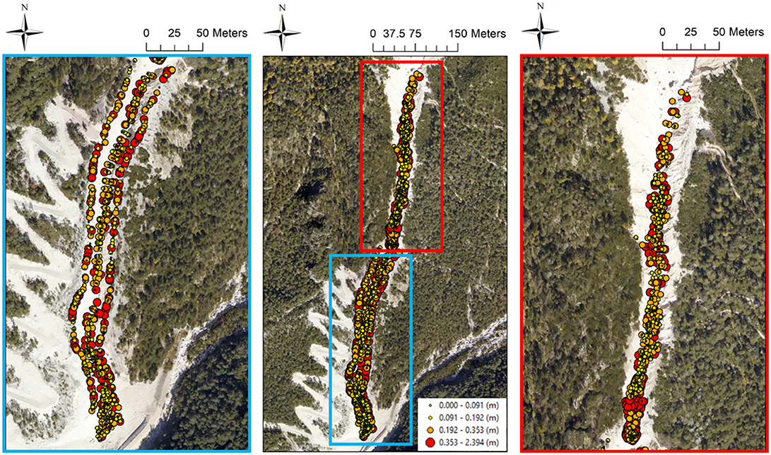
Figure 5. Choropleth symbol map of the thin-plate spline function absolute errors (spatial resolution of 1.00 m). Note that the greatest absolute errors mainly occur at the top of the banks and in the rough upper part of the study area. Within the channel the spatial pattern of errors appears to be “random”.

FIGURE 6

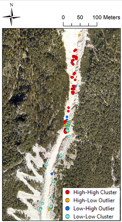
Figure 6. Local Moran's I index map of the thin-plate spline function absolute errors (spatial resolution of 1.00 m). Note the local clusters of high and low errors values mainly located along the upper part of the channel where the topographic roughness is higher due to the presence of boulders and bank failures. Furthermore, local outliers concentrate near the rock step at an altitude of about 1,500 m a.s.l.

The results of the interpolation algorithms robustness analysis in terms of NMAD and median of the vertical errors values variation on the basis of the sample density are summarized in Figure 7. The graphs of Figures 7A,B can be divided in two distinct regions. The first region (continuous border line) includes the interpolation algorithms which are stable (or robust) in relation to the sample density (i.e., the NMAD value does not change as the number of points used in the interpolation procedure decreases). Conversely, the second one (dotted border line) includes the routines whose prediction accuracy changes according to the sample density (the only exception is the ANUDEM algorithm, which provides consistent NMAD values). Furthermore, in the two delineated regions the spread of the NMAD values for each sample density differs. As a matter of fact, in the first region the spread of the values is smaller than that of the values in the second one, meaning that the interpolators within the first region yield similar accuracy values at each sample density. For both the chosen spatial resolutions, the thin-plate spline and multi-quadratic basis functions yield the more consistent NMAD values, which are also the lowest for each sample density. They are followed by the TIN-based interpolation algorithms and the Inverse Distance to a Power method. Conversely, at both the grid cell sizes, the ordinary kriging algorithm and the inverse multi-quadratic radial basis function are the least robust interpolation algorithms, along with the completely regularized spline function (only at the spatial resolution of 0.50 m). Furthermore, the graphs of Figures 7C,D highlight that all the tested gridding methods yield consistent vertical biases (i.e., the median of the vertical errors does not significantly change according to the sample density). The only exception is the ordinary kriging algorithm, which also provides positive median values (up to 0.10 m at a sample density equal to 50%). It is worth noting out that at the lowest sample densities (i.e., 75 and 50%) the kriging algorithm performs worst in terms of both systematic and random vertical error. This evidence is clearly in contrast with what reported in McDonnell and Lloyd (2015), who stated that for irregular spatial fields as the sample density decreases the kriging algorithm outperforms the deterministic interpolation methods.

FIGURE 7

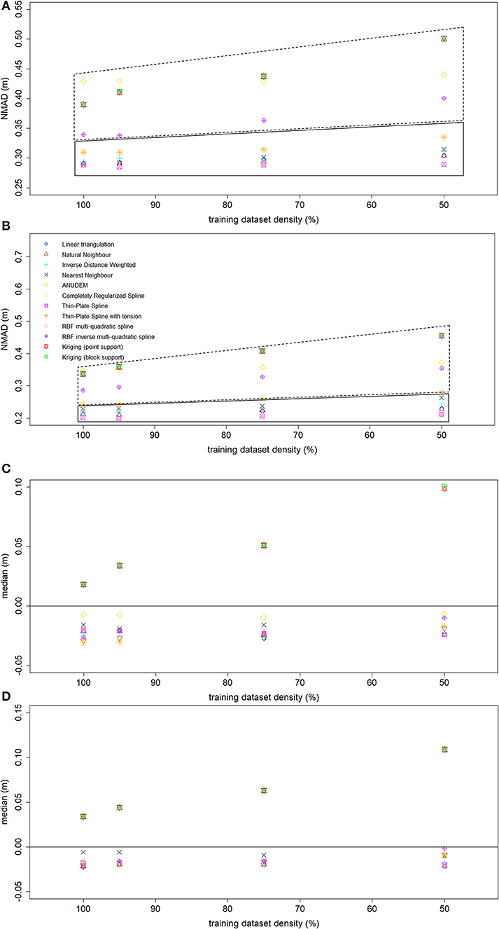
Figure 7. NMAD values variation as a function of the sample density (A, spatial resolution equal to 1.00 m, and B, spatial resolution equal to 0.50 m). Median values variation as a function of the sample density (C, spatial resolution equal to 1.00 m, and D, spatial resolution equal to 0.50 m).

The visual inspection carried out on the DEMs derivatives highlights that all the generated gridded surfaces contain noticeable interpolation artifacts (e.g., triangular facets; spiky features; striping effect; undulating, noisy, or over-smoothed relief; and discontinuos spatial pattern of slope and curvature), regardless of both the points density of the dataset used during the interpolation procedure and the chosen raster grid cell size (Figure 8). However, for the linear triangulation, natural neighbor, ANUDEM, completely regularized spline, thin-plate spline plus tension, and ordinary kriging algorithms, they do not prevent an overall satisfactory visual representation of the channel morphology. Conversely, the Inverse Distance to a Power, nearest neighbor, and inverse multi-quadratic basis function algorithms yield overly noisy DEMs. Furthermore, despite their excellent statistical performance, also the thin-plate spline and multi-quadratic radial basis functions do not ensure a realistic representation of the study site topography mainly due to function under- and over-shooting. As a consequence, relevant spiky features in correspondence of slope discontinuities are generated, both internally and externally to the channel area (Figure 8A). This finding endorses the importance of integrating statistical and qualitative techniques when an interpolation algorithm performance analysis is undertaken, as suggested by a number of earlier studies (e.g., Wood and Fisher, 1993; Declercq, 1996; Wood, 1996; Desmet, 1997; Yang and Hodler, 2000; Chaplot et al., 2006; Podobnikar, 2009; Setiawan et al., 2013). The multi-criteria morphological based comparison points out that the completely regularized spline and the thin-plate spline plus tension functions ensure the most realistic plano-altimetric representation of both longitudinal and transversal linear features, both channel bottom forms. Conversely, the ANUDEM and ordinary kriging methods prove the lowest shape reliability mainly due to surface over-smoothing, with slope discontinuities and channel bottom forms not well defined in the corresponding DEMs. Moreover, a meaningful striping effect perpendicular to the trend direction (i.e., along the considered variogram modeling direction) affecting the kriging-derived DEMs suggests that the methodology here followed to kridge the LiDAR points dataset does not represent a suitable procedure to interpolate DEMs for hydrological and hydraulic modeling (Figure 8C). The linear triangulation and the natural neighbor algorithm perform in an intermediate position, with an overall realistic representation of channel features although the contours in some cases appear irregular or with spurious shapes. The results of the residual analysis carried out on the full dataset-derived 0.50 meters-resolution DEMs are shown (as an example) in Figure 6S of the Supplementary Material. It turns out that the ANUDEM algorithm has the lowest ability to fulfill the topographic sampled data, followed by the ordinary kriging algorithm. On the other hand, no significant differences in the ability of honoring the sampled topographic data are detected among the remaining tested gridding methods.

FIGURE 8

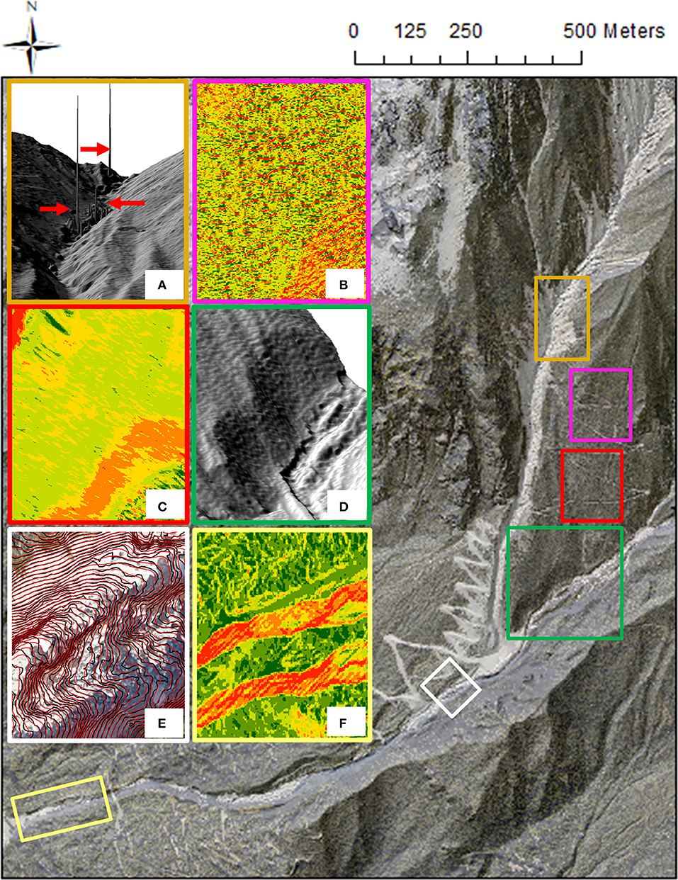
Figure 8. Overview of the detected interpolation artifacts: (A) spiky features in the upper part of the debris flow channel due to function under- and over-shooting in correspondence of slope discontinuities, (B) noisy relief with a discontinuos spatial pattern of slopes, (C) striping effect oriented according to the direction of variogram modeling, (D) undulating surface, (E) over-smoothed surface (red lines: 1-meter interval contour lines of the ANUDEM-derived DEM, black lines: 1-meter interval contour lines of the natural neighbor-derived DEM), (F) striping effect oriented according to the sampling direction.

Effects of the Gridding Techniques on Debris Flow Routing Modeling

For the two modeled event scenarios (i.e., 50 and 300-years return periods), the results of the global (i.e., at the channel extent) correlation analysis between the pixel-wise standard deviation of the twelve full dataset-derived 1-meter resolution DEMs heights and the pixel-wise standard deviation of the corresponding twelve simulated erosion/deposition depths are summarized in Figures 9A,B, respectively. For both the event scenarios, the Pearson's and the Spearman's rank correlation coefficient approach similar low values, respectively equal to 0.13 and 0.21 (i.e., about 15–20% of the perfect positive correlation between the two analyzed variables). Only a slight improvement in the correlation strength is gained by using the 50% thinning-derived 1-meter resolution DEMs in the model runs (Figures 9C,D). Furthermore, also the moving windows correlation analysis does not emphasize a strong spatial link between the cells with high uncertainty in the simulated erosion/deposition depths and those with high uncertainty in the input topographic data (Figure 10), regardless of both the magnitude of the modeled event scenario and the points density of the dataset used during the interpolation procedure.

FIGURE 9

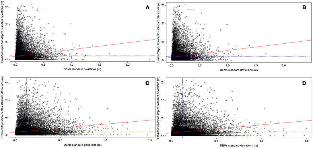
Figure 9. Scatterplot of the pixel-wise standard deviations of the twelve 1-meter resolution DEMs heights and the pixel-wise standard deviation of the corresponding twelve simulated erosion/deposition depths: (A) full dataset-derived DEMs and 300-years return period (rho Pearson = 0.126, rho Spearman = 0.205), (B) full dataset-derived DEMs and 50-years return period (rho Pearson = 0.129, rho Spearman = 0.208), (C) 50% thinning-derived DEMs and 300-years return period (rho Pearson = 0.167, rho Spearman = 0.252), and (D) 50% thinning-derived DEMs and 50-years return period (rho Pearson = 0.172, rho Spearman = 0.256). The continuous red line corresponds to the linear regression line, whereas the dotted blue lines correspond to the marginal mean of the two correlated variables.

FIGURE 10

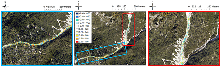
Figure 10. 5 × 5 moving windows Pearson's correlation coefficient between the pixel-wise standard deviations of the twelve 50% thinning-derived 1-meter resolution DEMs heights and the pixel-wise standard deviation of the corresponding twelve 50-years return period simulated erosion/deposition depths.

For the 50% thinning-derived 1-meter resolution DEMs, we report (as an example) the 50-years return period run results in terms of: simulated erosion/deposition areas and volumes (Table 4), solid-liquid discharges (Figure 11), and channel morphology after the event (Figure 12). Overall, the results do not highlight a noteworthy change in the routing model behavior depending on the used topographic surface, regardless of both the magnitude of the modeled event scenario and the points density of the dataset used during the interpolation procedure. In detail, in Table 4 the spread of the simulated flooded area values is smaller than 2,000 m² (i.e., smaller than 10% of the mean of all the simulated flooded area values), whereas for the simulated erosion and deposition areas it corresponds to 854 m² (i.e., 7% of the mean of all the simulated erosion area values) and 1,191 m² (i.e., 6% of the mean of all the simulated deposition area values), respectively. Similarly, the spread of the simulated erosion and deposition volume values is equal to 6,166 m³ (i.e., 14% of the mean of all the simulated erosion volume values) and 3,217 m³ (i.e., 13% of the mean of all the simulated deposition volume values), respectively. Clearly, these differences can be regarded as negligible when the cell routing model is used at forecasting purposes, or to identify the areas mainly subjected to large erosion and deposition phenomena. The solid-liquid hydrographs shown in Figure 11 relate to two cross-sections located in the upper part of the channel, just downstream the triggering area of the Rovina di Cancia debris flow. All the hydrographs show a comparable well-defined triangular shape with similar values of peak discharge, time to peak, and duration. It means that the dynamic of the simulated flow is not strongly influenced by the topographic uncertainty due to the different tested interpolation algorithms. This finding is also confirmed by the cross-section profiles of the pre- (continuous line) and post-event (dotted lines) DEMs shown in Figure 12. The reported cross-section profiles are representative of a channel reach mainly subject to erosion processes (Figure 12A), deposition processes (Figure 12B), and mixed erosion and deposition processes (Figure 12C). For all the cross-sections, the DEMs profiles do not highlight meaningful differences in the channel morphology after the event. Even more important, the detected differences in the erosion and deposition profiles do not appear to be linked to the profiles variability of the input DEMs.

TABLE 4

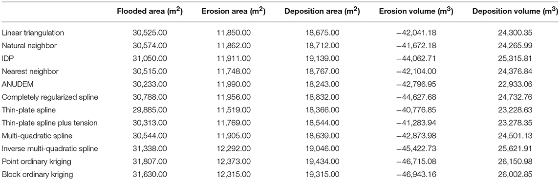
Table 4. 50% thinning-derived 1-meter resolution DEMs model run results (50-years return period).

FIGURE 11

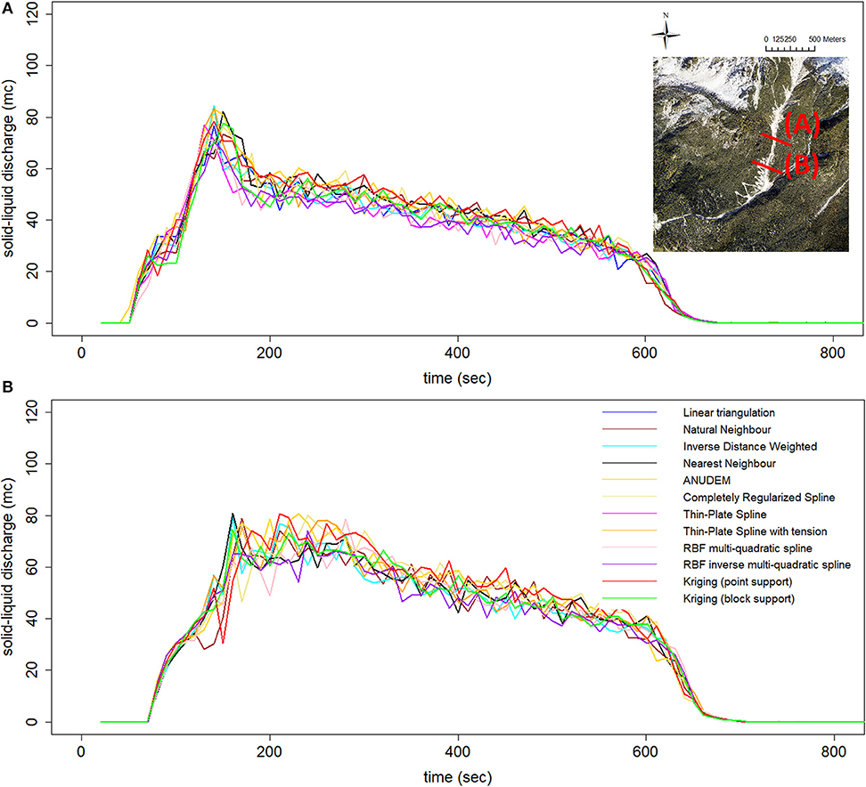
Figure 11. Comparison of the simulated debris flow solid-liquid hydrographs (A, upstream section, and B, downstream section).

FIGURE 12

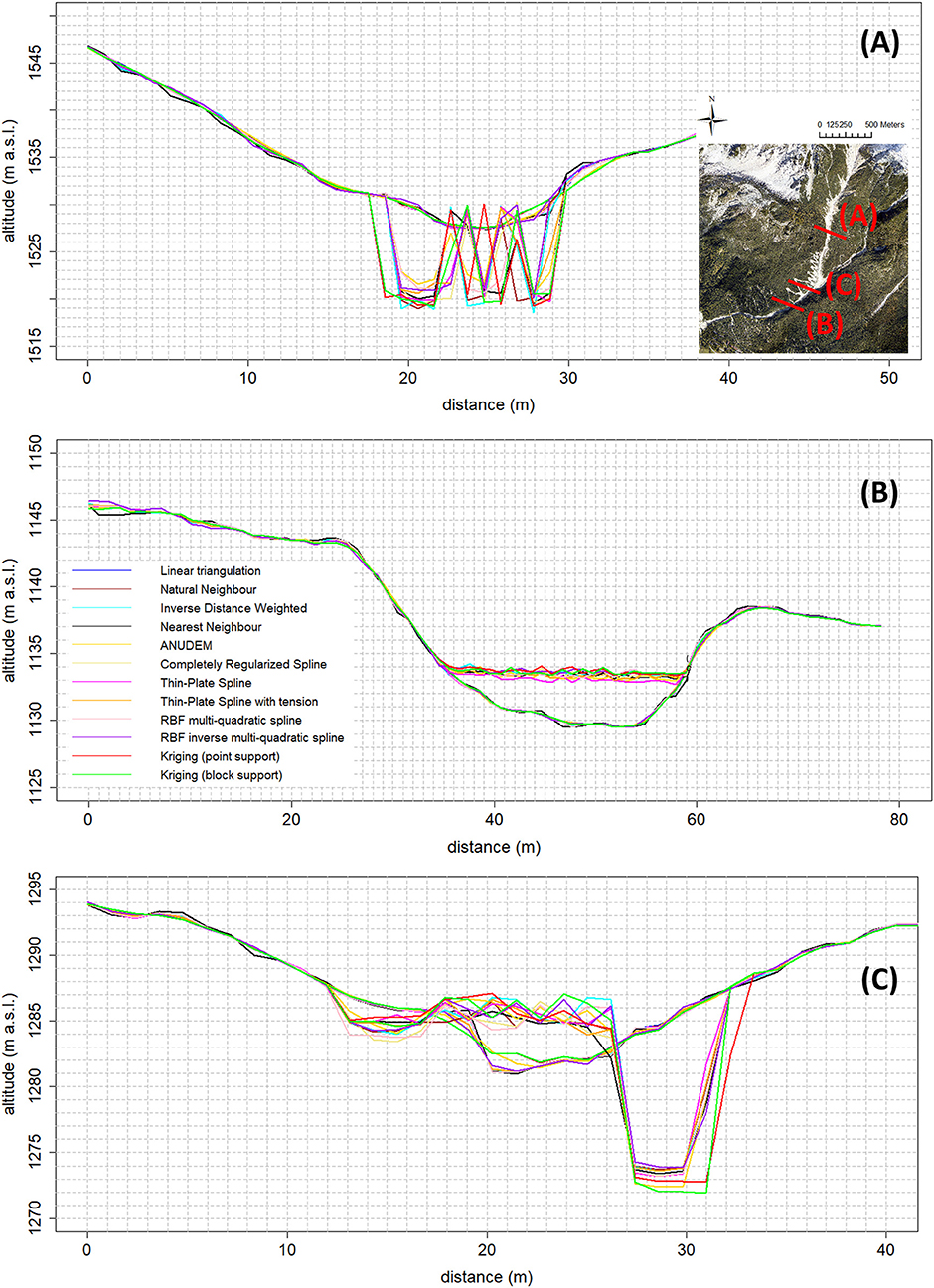
Figure 12. Comparison of the pre- (continuous lines) and post-event (dotted lines) DEMs cross-section profiles (erosional (A), depositional (B), and mixed erosional-depositional reach (C) of the Rovina di Cancia debris flow channel).

Conclusions

In this study we compared the performance of twelve gridding algorithms (i.e., linear triangulation, natural neighbor, nearest neighbor, Inverse Distance to a Power, ANUDEM, completely regularize spline function, thin-plate spline function, thin-plate spline plus tension function, multi-quadratic function, inverse multi-quadratic function, point ordinary kriging, and block ordinary kriging) in building DEMs with the complex topography of a debris flow channel located in the Venetian Dolomites. After that, we paid special attention in assessing the relationship existing between the digital elevation uncertainty due to the use of the different tested interpolation methods and the uncertainty on the results of a GIS-based cell model for simulating stony debris flows routing.

The investigation carried out on the performance of the tested interpolation algorithms highlighted that the ordinary kriging algorithm, applied according to the followed methodology (i.e., employing a theoretical variogram model fitted on the directional empirical one computed perpendicularly to the linear global trend), is not suitable for reproducing the complex topography of the debris flow channel. As a matter of fact, it has demonstrated an overall unsatisfactory statistical performance, a low robustness, and a poor shape reliability. Also the ANUDEM algorithm has exhibited an overall unsatisfactory performance (from both the quantitative and qualitative point of view), despite it represents the only tested interpolation method specifically intended for digital terrain modeling. Conversely, the thin-plate spline function proved to be the most accurate and stable interpolation algorithm, along with the multi-quadratic radial basis function. However, they have demonstrated a low ability in faithfully representing the shape of the channel, mainly due to function under- and over-shooting causing relevant spiky features in correspondence of slope discontinuities. This lead to the conclusion that when the absolute accuracy of the elevation values is the most important feature, these algorithms could represent the best choice also in natural landscapes featuring a high morphological complexity. On the other hand, when also the realistic representation of surface shape is important, the linear triangulation, the natural neighbor algorithm, and the thin-plate spline plus tension and completely regularized spline basis functions could represent a better choice, since they ensure a proper trade-off among accuracy and shape reliability.

The evaluation of the effects of the gridding techniques on debris flows routing modeling revealed that the correlation between the uncertainty in the cell elevations due to the different tested interpolation methods and the uncertainty in the corresponding simulated erosion/deposition depths was weak, regardless of both the magnitude of the modeled event scenario and the points density of the dataset used during the interpolation procedure. Also the results of the different model runs in terms of simulated areas, erosion and deposition volumes, solid-liquid discharges, and channel morphology after the event did not highlight a significant change in the model behavior depending on the used topographic surface. This leads to the conclusion that the choice of the interpolation algorithm does not represent a determining factor for debris flows routing modeling.

However, the extrapolation of the latter conclusion must be done with care at least for two reasons. In fact, the investigation was performed focusing on a channelized-debris flow, whose flow depths are larger than the DEMs height uncertainty resulting from the interpolation procedure. So, future researches have to be carried out in order to test the influence of the gridding algorithms on non-channelized debris flows, since in this case small interpolation errors might have a greater impact on the dynamic of the simulated flow, and thus on the resulting erosional/depositional pattern. Furthermore, also the use of different rheological models and/or sediments erosion and deposition process schematizations might lead to different conclusions. Therefore, in order to confirm the finding of this paper more work has to be done also by testing different debris flows routing models.

Author Contributions

MBo carried out the analysis on the topographic data, the interpolation of DEMs, the comparison among the different gridding routine, the numerical simulations, and the analysis on the obtained results. MBe carried out the hydrological simulations, performed the rtkGPS surveys, and helped building a code for GIS analysis. CG contributed to the triggering and hydraulic simulations. Furthermore, he, supervised, checked, and reviewed the work.

Conflict of Interest Statement

The authors declare that the research was conducted in the absence of any commercial or financial relationships that could be construed as a potential conflict of interest.

Acknowledgments

The authors wish to thank the Regional Civil Work Agency of Veneto for the ortho-photos and full-waveform LiDAR data. We also thank the Environmental Protection Agency of Veneto (ARPAV) for providing the meteorological data used in the hydrological modeling. Data are available under request to the corresponding author.

Supplementary Material

The Supplementary Material for this article can be found online at: https://www.frontiersin.org/articles/10.3389/feart.2018.00089/full#supplementary-material

Abbreviations

DEM(s), Digital Elevation Model(s); LiDAR, Light Detection And Ranging; GIS, Geographic Information Systems; TIN(s), Triangulated Irregular Network(s); IDP, Inverse Distance to a Power function; RBFs, Radial Basis Functions; ALS, Airborne Laser Scanner; GPS, Global Positioning System; RTK-GPS, Real-Time Kinematic GPS; ESDA, Exploratory Spatial Data Analysis; NMAD, Normalized Median of Absolute Deviations; RMSE, Root Mean Square Error; MAE, Mean Absolute Error.

Footnotes

1. ^Nominal conversion accuracy equal to ±0.035 m at 1σ.

2. ^Isenburg, M. (2017). LAStools - efficient LiDAR processing software (version 170608, unlicensed).

References

Aguilar, F. J., Agüera, F., Aguilar, M. A., and Carvajal, A. F. (2005). Effects of Terrain Morphology, Sampling Density, and Interpolation Methods on Grid DEM Accuracy. Photogram. Eng. Remote Sens. 71, 805–816. doi: 10.14358/PERS.71.7.805

CrossRef Full Text | Google Scholar

Armanini, A., Fraccarollo, L., and Rosatti, G. (2009). Two-dimensional simulation of debris flows in erodible channels. Comput. Geosci. 35, 993–1006. doi: 10.1016/j.cageo.2007.11.008

CrossRef Full Text | Google Scholar

Bater, C. W., and Coops, N. C. (2009). Evaluating error associated with lidar-derived DEM interpolation. Comput. Geosci. 35, 289–300. doi: 10.1016/j.cageo.2008.09.001

CrossRef Full Text | Google Scholar

Berger, C., McArdell, B. W., and Schlunegger, F. (2011). Direct measurement of channel erosion by debris flows, Illgraben, Switzerland. J. Geophys. Res. 116:F01002. doi: 10.1029/2010JF001722

CrossRef Full Text | Google Scholar

Berti, M., Genevois, R., Simoni, A., and Tecca, R. P. (1999). Field observations of a debris flow event in the Dolomites. Geomorphology 29, 265–274. doi: 10.1016/S0169-555X(99)00018-5

CrossRef Full Text | Google Scholar

Berti, M., and Simoni, A. (2005). Experimental evidences and numerical modeling of debris flow initiated by channel runoff. Landslides 2, 171–182. doi: 10.1007/s10346-005-0062-4

CrossRef Full Text | Google Scholar

Berti, M., and Simoni, A. (2014). DFLOWZ: a free program to evaluate the area potentially inundated by a debris flow. Comput. Geosci. 67, 14–23. doi: 10.1016/j.cageo.2014.02.002

CrossRef Full Text | Google Scholar

Blöschl, G., and Grayson, R. (2000). Spatial Observations and Interpolation. Spat. Patt. Catch. Hydrol. 113, 13–16.

Google Scholar

Bossi, G., Cavalli, M., Crema, S., Frigerio, S., Luna, B. Q., and Mantovani, M. (2014). Multi temporal LiDAR-DTMs as a tool for modeling a complex landslide: a case study in the Rotolon catchment (Eastern Italian Alps). Natl. Hazards Earth Syst. Sci. Discus. 2, 6453–6474. doi: 10.5194/nhessd-2-6453-2014

CrossRef Full Text | Google Scholar

Caroti, G., and Piemonte, A. (2010). Analisi Dei Dati Altimetrici Disponibili Per Il Territorio Comunale Di Pisa, Geomatica le Radici Del Futuro. Pavia: Edizioni SIFET.

Carrara, A., Bitelli, G., and Carla, R. (1997). Comparison of techniques for generating digital terrain models from contour lines. Int. J.Geogr. Inform. Sci. 11, 451–472. doi: 10.1080/136588197242257

CrossRef Full Text | Google Scholar

Cavalli, M., and Marchi, L. (2008). The effectiveness of airborne LiDAR's data in the recognition of channel-bed morphology. Catena 75, 249–260. doi: 10.1016/j.catena.2007.11.001

CrossRef Full Text | Google Scholar

Chaplot, V., Darboux, F., Bourennane, H., Leguedois, S., Silvera, N., and Phachomphon, K. (2006). Accuracy of interpolation techniques for the derivation of digital elevation models in relation to landform types and data density. Geomorphology 77, 126–141. doi: 10.1016/j.geomorph.2005.12.010

CrossRef Full Text | Google Scholar

Chiles, J. P. (1984). “Simulation of a nickel deposit: problems encountered and practical solutions,” in Geostatistics for Natural Resources Charucterization, eds G. Verly, M. David, A. G. Journel, and A. Makchal. Dordrecht; Hollan: Reidel, Springer.

Google Scholar

Cilloccu, F., Dequal, S., Brovelli, M., Crespi, M., and Lingua, A. (2009). Ortoimmagini 1:10.000 e modelli altimetrici. Linee Guida. Roma: CISIS - Centro Interregionale per i Sistemi Informatici, Geografici e Statistici.

Google Scholar

Deangeli, C. (2008). Laboratory granular flows generated by slope failures. Rock Mech. Rock Eng. 41, 199–217. doi: 10.1007/s00603-007-0131-1

CrossRef Full Text | Google Scholar

Declercq, F. A. N. (1996). Interpolation methods for scattered sample data: accuracy, spatial patterns, processing time. Cartogr. Geogr. Inform. Sys. 23, 128–144. doi: 10.1559/152304096782438882

CrossRef Full Text | Google Scholar

Degetto, M., Gregoretti, C., and Bernard, M. (2015). Comparative analysis of the differences between using LiDAR and contour-based DEMs for hydrological modeling of runoff generating debris flows in the Dolomites. Front. Earth Sci. 3:21. doi: 10.3389/feart.2015.00021

CrossRef Full Text | Google Scholar

Desmet, P. J. J. (1997). Effects of interpolation errors on the analysis of DEMs. Earth Surf. Process. Landforms 22, 563–580. doi: 10.1002/(SICI)1096-9837(199706)22:6<563::AID-ESP713>3.0.CO;2-3

CrossRef Full Text | Google Scholar

Di Cristo, C., Iervolino, M., and Vacca, A. (2014). Applicability of kinematic, diffusion and quasi-steady dynamic wave models to shallow mud flows. J. Hydrol. Eng. 19, 956–965. doi: 10.1061/(ASCE)HE.1943-5584.0000881

CrossRef Full Text | Google Scholar

Easterling, D. R., Evans, J. L., Groisman, P. Y., Karl, T. R., Kunkel, K. E., and Ambenje, P. (2000). Observed variability and trends in extreme climate events: a brief review. Bull. Am. Meteorol. Soc. 81, 417–425. doi: 10.1175/1520-0477(2000)081<0417:OVATIE>2.3.CO;2

CrossRef Full Text | Google Scholar

Egashira, S., and Ashida, K. (1987). “Sediment transport in steep slope flumes,” in Proceedings of Roc Japan Joint Seminar on Water Resources.

Google Scholar

El-Sheimy, N., Valeo, C., and Habib, A. (2005). Digital Terrain Modeling Acquisition, Manipulation, and Applications; Artech House: Boston, MA.

Erdogan, S. (2009). A comparison of interpolation methods for producing digital elevation models at the field scale. Earth Surf. Proc. Land. 34, 366–376. doi: 10.1002/esp.1731

CrossRef Full Text | Google Scholar

Evans, J. S. (2017). SpatialEco. R package version 0.0.1-7. Available online at: https://CRAN.R-project.org/package=spatialEco

Floris, M., D'Alpaos, A., Squarzoni, C., Genevois, R., and Marani, M. (2010). Recent changes in rainfall characteristics and their influence on thresholds for debris flow triggering in the Dolomitic area of Cortina d'Ampezzo, north-eastern Italian Alps. Nat. Hazards Earth Syst. Sci. 10, 571–580. doi: 10.5194/nhess-10-571-2010

CrossRef Full Text | Google Scholar

Fonstad, M. A., Dietrich, J. T., Courville, B. C., Jensen, J. L., and Carbonneau, P. E. (2013). Topographic structure from motion: a new development in photogrammetric measurement. Earth Surface Proces. Landf. 38, 421–430. doi: 10.1002/esp.3366

CrossRef Full Text | Google Scholar

French, J. R. (2003). Airborne LiDAR in support of geomorphological and hydraulic modeling. Earth Surf. Process. Landf. 28, 321–335. doi: 10.1002/esp.484

CrossRef Full Text | Google Scholar

Gallay, M., Lloyd, C. D., McKinley, J., and Barry, L. (2013). Assessing modern ground survey methods and airborne laser scanning for digital terrain modeling: a case study from the Lake District, England. Comput. Geosci. 51, 216–227. doi: 10.1016/j.cageo.2012.08.015

CrossRef Full Text | Google Scholar

Garnero, G., and Godone, D. (2011). Accuratezza Nell'interpolazione dei DTM: Analisi dei fattori Determinanti. Colorno: Atti del XV Conferenza Nazionale ASITA.

Google Scholar

Ghilardi, P., Natale, L., and Savi, F. (2001). Modeling debris-flow propagation and deposition. Phys. Chem. Earth C 26, 651–656. doi: 10.1016/S1464-1917(01)00063-0

CrossRef Full Text | Google Scholar

Gregoretti, C., and Dalla Fontana, G. (2007). “Rainfall threshold for the initiation of debris flows by channel bed failure of the dolomites,” in Proceedings of the Fourth International Conference on Debris Flow Hazards Mitigation, eds C. L. Chen and J. J. Major (Chengdu: Balkema), 11–21.

Google Scholar

Gregoretti, C., and Dalla Fontana, G. (2008). The triggering of debris flow due to channel-bed failure in some alpine headwater basins of the Dolomites: analyses of critical runoff. Hydrol. Process. 22, 2248–2263. doi: 10.1002/hyp.6821

CrossRef Full Text | Google Scholar

Gregoretti, C., Degetto, M., Bernard, M., and Boreggio, M. (2018b). The debris flow occurred at Ru Secco Creek, Venetian Dolomites, on 4 August 2015: analysis of the phenomenon, its characteristics and reproduction by models. Front. Earth Sci. 6:367817. doi: 10.3389/feart.2018.00080

CrossRef Full Text | Google Scholar

Gregoretti, C., Degetto, M., Bernard, M., Crucil, G., Pimazzoni, A., De Vido, G., et al. (2016b). Runoff of small rocky headwater catchments: Field observations and hydrological modeling. Water Resour. Res. 52, 8138–8158. doi: 10.1002/2016WR018675

CrossRef Full Text | Google Scholar

Gregoretti, C., Degetto, M., and Boreggio, M. (2016a). GIS-based cell model for simulating debris flow runout on a fan. J. Hydrol. 534, 326–340. doi: 10.1016/j.jhydrol.2015.12.054

CrossRef Full Text | Google Scholar

Gregoretti, C., Stancanelli, L., Bernard, M., Degetto, M., Boreggio, M, and Lanzoni, S (2018a). Relevance of erosion processes when modelling in-channel gravel debris flows for efficient hazard assessment. J. Hydrol. doi: 10.1016/j.jhydrol.2018.10.001

CrossRef Full Text | Google Scholar

Hancock, G. R. (2006). The impact of different gridding methods on catchment geomorphology and soil erosion over long timescales using a landscape evolution model. Earth Surf. Process. Landforms 31, 1035–1050. doi: 10.1002/esp.1306

CrossRef Full Text | Google Scholar

Hengl, T. (2006). Finding the right pixel size. Comput. Geosci. 32, 1283–1298. doi: 10.1016/j.cageo.2005.11.008

CrossRef Full Text | Google Scholar

Hengl, T., and Reuter, H. I.(eds.). (2009). Geomorphometry: Concepts, Software, Applications. Developments in Soil Science, Vol. 33. Amsterdam; Oxford, UK: Elsevier.

Google Scholar

Heritage, G. L., and Large, A. R. G. (2009). Laser Scanning for the Environmental Sciences. London: Wiley-Blackwell.

Google Scholar

Heritage, G. L., Milan, D. J., Large, A. R. G., and Fuller, I. (2009). Influence of survey strategy and interpolation model upon DEM quality. Geomorphology 112, 334–344. doi: 10.1016/j.geomorph.2009.06.024

CrossRef Full Text | Google Scholar

Hodgson, M. E., and Bresnahan, P. (2004). Accuracy of Airborne Lidar-Derived Elevation. Photogram. Eng. Remote Sens.70, 331–339. doi: 10.14358/PERS.70.3.331

CrossRef Full Text | Google Scholar

Höhle, J., and Höhle, M. (2009). Accuracy assessment of digital elevation models by means of robust statistical methods. ISPRS J. Photogramm. Remote Sens. 64, 398–406. doi: 10.1016/j.isprsjprs.2009.02.003

CrossRef Full Text | Google Scholar

Höhle, J., and Potuckova, M. (2011). Assessment of the Quality of Digital Terrain Models. Amsterdam: European Spatial Data Research, Official Publication n. 60.

Hussin, H. Y., Quan Luna, B., van Westen, C. J., Christen, M., Malet, J. P., and van Asch Th, W. J (2012). Parameterization of a numerical 2-D debris flow model with entrainment: a case study of the Faucon catchment, Southern French Alps. Nat. Hazards Earth Syst. Sci. 12, 3075–3090. doi: 10.5194/nhess-12-3075-2012

CrossRef Full Text | Google Scholar

Hutchinson, M. F. (1996). “A locally adaptive approach to the interpolation of digital elevation models,” in Proceedings, Third International Conference/Workshop on Integrating GIS and Environmental Modeling, Santa Fe, NM, January 21-26, 1996 (Santa Barbara, CA: National Center for Geographic Information and Analysis).

Google Scholar

Isaaks, E. H., and Srivastava, R. M. (1989). An Introduction to Applied Geostatistics. Oxford: Oxford University Press.

Google Scholar

Iverson, R. M. (2005). “Debris-flow mechanics,” in Debris-Flow Hazards and Related Phenomena, eds M. Jakob and O. Hungr (Berlin; Heidelberg: Springer-Praxis), 105–134.

Google Scholar

Jaboyedoff, M., Oppikofer, T., Abellán, A., Derron, M. H., Loye, A., Metzger, R., et al. (2012). Use of LIDAR in landslide investigations: a review. Natl. Hazards 61, 5–28. doi: 10.1007/s11069-010-9634-2

CrossRef Full Text | Google Scholar

Johnston, K., Ver Hoef, J., Krivoruchko, K., and Neil, L. (2001). Using Arcgis Geostatistical Analyst. Redlands, CA: ESRI Press.

Google Scholar

Krause, P., Boyle, D. P., and Bäse, F. (2005). Comparison of different efficiency criteria for hydrological model assessment. Adv. Geosci. 5, 89–97. doi: 10.5194/adgeo-5-89-2005

CrossRef Full Text | Google Scholar

Lenzi, M. A., D'Agostino, V., Gregoretti, C., and Sonda, D. (2003). “A simplified numerical model for debris-flow hazard assessment: DEFLIMO,” in Third International Conference On Debris Flow Hazard Mitigations: Mechanics, Prediction and Assessment (Davos), 10–12.

Google Scholar

Li, Z. (1993). Theoretical models of the accuracy of digital terrain models: an evaluation and some observations. Photogram. Record 14, 651–660. doi: 10.1111/j.1477-9730.1993.tb00775.x

CrossRef Full Text | Google Scholar

Mallet, C., and Bretar, F. (2009). Full-waveform topographic LiDAR: state-of-the-art. ISPRS J. Photogram. Remote Sensing 64, 1–16. doi: 10.1016/j.isprsjprs.2008.09.007

CrossRef Full Text | Google Scholar

Mattea, S., Franceschinis, C., Scarpa, R., and Thiene, M. (2016). Valuing landslide risk reduction programs in the Italian Alps: the effect of visual information on preference stability. Land Use Policy 59, 176–184. doi: 10.1016/j.landusepol.2016.08.032

CrossRef Full Text | Google Scholar

McDonnell, R. A., and Lloyd, C. D. (2015). Principles of Geographical Information Systems. Oxford, UK: Oxford University Press.

Google Scholar

Medina, V., Hurlimann, M., and Bateman, A. (2008). Application of FLATModel, a 2D finite volume code, to debris flows in the Northeastern part of Iberian Peninsula Experimental evidences and numerical modeling of debris flow initiated by channel runoff. Landslide 5, 127–142. doi: 10.1007/s10346-007-0102-3

CrossRef Full Text | Google Scholar

Milan, D. J., Heritage, G. L., Large, A. R. G., and Fuller, I. C. (2011). Filtering spatial error from DEMs: implications for morphological change estimation. Geomorphology 125, 160–171. doi: 10.1016/j.geomorph.2010.09.012

CrossRef Full Text | Google Scholar

Mitas, L., and Mitasova, H. (1999). Spatial interpolation. Geogr. Inf. Syst. Principles Tech. Manag. Appl. 1, 481–492.

Google Scholar

Moore, I. D., and Grayson, R. B. (1991). Terrain-based catchment partitioning and runoff prediction using vector elevation data. Water Resour. Res. 27, 1177–1191. doi: 10.1029/91WR00090

CrossRef Full Text | Google Scholar

Oliver, M. A., and Webster, R. (2014). Catena A tutorial guide to geostatistics: computing and modeling variograms and kriging. Catena 113, 56–69. doi: 10.1016/j.catena.2013.09.006

CrossRef Full Text | Google Scholar

Pfeifer, N. (2005). A subdivision algorithm for smooth 3D terrain models. ISPRS J. Photogram. Remote Sensing 59, 115–127. doi: 10.1016/j.isprsjprs.2004.09.002

CrossRef Full Text | Google Scholar

Podobnikar, T. (2009). Methods for visual quality assessment of Digital Terrain Model. J. SAPIENS 2, 15–24.

Google Scholar

Pourali, S., Arrowsmith, C., and Chrisman, N. (2014). “Vertical accuracy assessment of LiDAR ground points using minimum distance approach,” in Research at Locate'14, eds S. Winter and C. Rizos (Canberra, ACT: Rheinisch-Westfaelische Technische Hochschule Aache), 86–96.

Google Scholar

R Development Core Team (2008). R: A Language and Environment for Statistical Computing. Vienna: R Foundation for Statistical Computing.

Reutebuch, S. E., McGaughey, R. J., Andersen, H. E., and Carson, W. W. (2003). Accuracy of a high-resolution lidar terrain model under a conifer forest canopy. Can. J. Remote Sensing 29, 527–535. doi: 10.5589/m03-022

CrossRef Full Text | Google Scholar

Rickenmann, D., Laigle, B., McArdell, B. W., and Hubl, J. (2006). Comparison of 2D debris-flow simulation models with field events. Comput. Geosci. 10, 241–264 doi: 10.1007/s10596-005-9021-3

CrossRef Full Text | Google Scholar

Rosatti, G., and Begnudelli, L. (2013). Two-dimensional simulation of debris flows over mobile bed: enhancing the TRENT2D model by using a well-balanced generalized Roe-type solver. Comput. Fluids 71, 179–185. doi: 10.1016/j.compfluid.2012.10.006

CrossRef Full Text | Google Scholar

Saksena, S., and Merwade, V. (2015). Incorporating the effect of DEM resolution and accuracy for improved flood inundation mapping. J. Hydrol. 530, 180–194. doi: 10.1016/j.jhydrol.2015.09.069

CrossRef Full Text | Google Scholar

Scheidl, C., and Rickenmann, D. (2010). “TopFlowDF-A simple GIS based model to simulate debris-flow runout on the fan,” in Proceedings of the Fifth International Conference on Debris Flow Hazards Mitigation (Padova), 253–262.

Google Scholar

Scheidl, C., Rickenmann, D., and Chiari, M. (2008). The use of airborne LiDAR data for the analysis of debris flow events in Switzerland. Nat. Hazards Earth Syst. Sci. 8, 1113–1127. doi: 10.5194/nhess-8-1113-2008

CrossRef Full Text | Google Scholar

Schwendel, A. C., Fuller, I. C., and Death, R. G. (2012). Assessing DEM interpolation methods for effective representation of upland stream morphology for rapid appraisal of bed stability. River Res. Applic. 28, 567–584. doi: 10.1002/rra.1475

CrossRef Full Text | Google Scholar

Setiawan, M. A., Rutzinger, M., Wichmann, V., Stoetter, J., and Sartohadi, J. (2013). Evaluation of Methods for Digital Elevation Model Interpolation of Tillage Systems. J. Natl. Resour. Develop. 3, 1 28–139. doi: 10.5027/jnrd.v3i0.13

CrossRef Full Text | Google Scholar

Simoni, A., Bernard, M., Berti, M., Boreggio, M., Lanzoni, S., Stancanelli, L. M., et al. (2018). “Observation of initiation conditions and role of sediment availability in run-off generated debris flows at Cancia (North Eastern Italian Alps),” in Geographical Research Abstract. Vol. 20, EGU2018-9091 (Vienna: EGU General Assembly 2018).

Google Scholar

Smith, S., Holland, D., and Longley, P. (2005). “The importance of understanding error in LiDAR digital elevation models,” 20 th ISPRS Conference (Istanbul), 12–34.

Google Scholar

Sodnik, J., Podobnikar, T., and Mikoš, M. (2012). “Using LiDAR data for debris flow modeling,” in 12th Congress INTERPRAEVENT 2012 (Grenoble), 573–583.

Google Scholar

Takahashi, T. (1978). Mechanical characteristics of debris flow. J. Hydr. Div. ASCE 104, 1153–1169.

Google Scholar

Takahashi, T. (2007). Debris Flow Mechanics, Prediction and Countermeasures. London; Leiden: Taylor and Francis, Balkema.

Google Scholar

Tarolli, P. (2014). High-resolution topography for understanding Earth surface processes: opportunities and challenges. Geomorphology 216, 295–312, doi: 10.1016/j.geomorph.2014.03.008

CrossRef Full Text | Google Scholar

Theule, J. I., Liebault, F., Loye, A., Laigle, D., and Jaboyedoff, M. (2012). Sediment budget monitoring of debris flow and bedload transport in the Manival Torrent, SE France. Natl. Hazard Earth Sci. 12, 731–749. doi: 10.5194/nhess-12-731-2012

CrossRef Full Text | Google Scholar

Thiene, M., Shaw, W. D., and Scarpa, R (2017). Perceived risks of mountain landslides in Italy: stated choices for subjective risk reductions. Landslides 14, 1077–1089. doi: 10.1007/s10346-016-0741-3

CrossRef Full Text | Google Scholar

Tiranti, D., and Deangeli, C. (2015). Modeling of debris flow depositional patterns according to the catchment and sediment source area characteristics. Front. Earth Sci. 3:8. doi: 10.3389/feart.2015.00008

CrossRef Full Text | Google Scholar

Tsubaki (1972). “Keikoku taiseki dosha no ryndo,” in XXVII Japanese National Congress on Civil Engineering (in japanese).

Vosselman, G. V., and Maas, H. G.(eds.). (2010). Airborne and Terrestrial Laser Scanning. Scotland, UK: Whittles.

Google Scholar

Wagner, W., Ullrich, A., Ducic, V., Melzer, T., and Studnicka, N. (2006). Gaussian decomposition and calibration of a novel small-footprint full-waveform digitising airborne laser scanner. ISPRS J. Photogramm. Remote Sens. 60, 100–112. doi: 10.1016/j.isprsjprs.2005.12.001

CrossRef Full Text | Google Scholar

Webster, T. L., and Dias, G. (2006). An automated GIS procedure for comparing GPS and proximal LIDAR elevations. Comput. Geosci. 32, 713–726. doi: 10.1016/j.cageo.2005.08.009

CrossRef Full Text | Google Scholar

Weng, Q. (2006). “An evaluation of spatial interpolation accuracy of elevation data,” in Progress in Spatial Data Handling, eds A. Riedl, W. Kainz, G. A. Elmes (Berlin: Springer-Verlag), 805–824.

Google Scholar

Wilson, J. P., and Gallant, J. C. (2000). “Digital terrain analysis,” in Terrain Analysis: Principles and Applications, eds J. P. Wilson and J. C. Gallant (New York, NY: Wiley), 1–28.

Google Scholar

Wise, S. M. (2000). Assessing the quality for hydrological applications of digital elevation models derived from contours. Hydrol. Process. 14, 1909–1929. doi: 10.1002/1099-1085(20000815/30)14:11/12<1909::AID-HYP45>3.0.CO;2-6

CrossRef Full Text | Google Scholar

Wise, S. M. (2007). Effect of differing DEM creation methods on the results from a hydrological model. Comput. Geosci. 33, 1351–1365. doi: 10.1016/j.cageo.2007.05.003

CrossRef Full Text | Google Scholar

Wood, J. D. (1996). The Geomorphological Characterisation of Digital Elevation Models. Unpublished Doctoral Thesis, University of Leicester.

Wood, J. D., and Fisher, P. F. (1993). Assessing Interpolation Accuracy in Elevation Models. IEEE Comput. Graph. Applic. 13, 48–56. doi: 10.1109/38.204967

CrossRef Full Text | Google Scholar

Yang, X., and Hodler, T. (2000). Visual and statistical comparisons of surface modeling techniques for point-based environmental data. Cartogr. Geogr. Inform. Sci. 27, 165–175. doi: 10.1559/152304000783547911

CrossRef Full Text | Google Scholar