Identifying Spatial Variability in Greenland's Outlet Glacier Response to Ocean Heat

1. Introduction

How the large ice sheets will respond to climatic forcing is important for projections of future ice loss. Some recent studies have found widespread change of the ice sheets (Seale et al., 2011), while others reveal a high degree of spatial and temporal variability of outlet glacier change (e.g., McFadden et al., 2011; Moon et al., 2012; Csatho et al., 2014). These complex patterns are illustrated in glacier accelerations (Rignot and Kanagaratnam, 2006), terminus retreat (Walsh et al., 2012), ice discharge (Howat et al., 2007), and rates of ice surface elevation change (e.g., Pritchard et al., 2009; Khan et al., 2013). Moon et al. (2012) show that within a region that is thinning on the whole, individual glaciers can be changing very differently from their neighbors. In light of such variability, applying trends observed at well-studied, fast changing glaciers to the remaining outlet glaciers likely overestimates future ice loss from the Greenland ice sheet.

This variable glacier change in Greenland makes it difficult to discern coherent patterns and assess the effect of proposed driving mechanisms. Here we use spatial statistical methods first to ascertain the global and local degree of spatial variability of tidewater glacier change, and then to investigate potential drivers of these patterns. Spatial autocorrelation describes the propensity for geographically close observations to co-vary, thus providing the first quantitative estimates of spatial randomness of glacier change. These methods have been developed for the objective interpretation of phenomena with a significant spatial component, such as cholera outbreaks (Giebultowicz et al., 2011) or cancer incidence rates proximal to coal-fired power plants (Mueller et al., 2015). These statistical tools are necessary to separate local glacier-to-glacier controls from the broader regionally-coherent glacier thinning signal.

For marine-terminating glaciers, variable behavior observed at adjacent glaciers may arise from differing fjord and ice geometry (Howat et al., 2007; Enderlin et al., 2013), sea ice and mélange buttressing (Amundson et al., 2010; Shepherd et al., 2012), subglacial discharge (Rignot and Kanagaratnam, 2006; Xu et al., 2012), micro-climates (Shepherd et al., 2009; Walsh et al., 2012), and dynamic interactions with the global ocean current system (Murray et al., 2010). In this paper, we will focus on one of these potential drivers of spatially-variable glacier change: the differential exposure to warm subsurface water in the fjord (Pritchard et al., 2009; Khan et al., 2013; Porter et al., 2014).

A flow-line model of Helheim Glacier by Nick et al. (2009) illustrates how terminus forcing impacts glacier mass balance through dynamic coupling; increased calving leads to grounding line retreat, glacier acceleration, and eventually a surface lowering signal that propagates inland (Truffer and Motyka, 2016). For marine-terminating glaciers, it is the delivery of heat to the ice face that is the primary control on subsurface melting. In Greenlandic fjords, the water below ~100–150 m deep is often Atlantic Water (AW) (Straneo et al., 2012), with high salinity and temperatures several degrees higher than the freezing point of seawater (typically S≥34.5, 0≥θ≥4°C). This increases the susceptibility of ice melt at depth (O'Leary and Christoffersen, 2013; Straneo et al., 2013), suggesting that a deeper grounding line and greater exposure to AW may lead to enhanced mass loss through undercutting of the ice face (Rignot et al., 2015).

One example of this bathymetry effect is seen for a pair of ~5 km wide outlet glaciers in NW Greenland, Tracy and Heilprin Glaciers. These neighboring glaciers show different patterns of change since the 2000's (Rignot and Kanagaratnam, 2006; Moon et al., 2012). Tracy Glacier has accelerated and thinned at elevated rates compared to Heilprin Glacier despite experiencing similar surface mass balance and far-field ocean conditions. Porter et al. (2014) find that for these two glaciers, a deeper grounding line and increased exposure to warm AW as the cause of differential glacial change.

For complex problems involving many difficult to measure, highly interconnected variables, statistical techniques have the ability to reveal and quantify key relationships. Here we use a combination of spatial analysis and linear regression methods to elucidate the complex patterns of glacier change.

2. Data

2.1. Glaciological Change

Surface elevation data from NASA Operation IceBridge (OIB) Airborne Topographic Mapper (ATM) and Land, Vegetation and Ice Sensor (LVIS) and the NASA ICESat mission have been combined into a spatially and temporally consistent dataset using the Surface Elevation Reconstruction and Change detection (SERAC) method for 1993–2012 (Csatho et al., 2014). Ice thickness changes derived from the SERAC ice sheet elevation time series for the ICESat period (2003–2009) provide the most comprehensive spatial and temporal coverage and provides the most consistent sampling across the Greenland Ice Sheet. Some portion of the ice thickness change derived from laser altimetry measurements can be attributed to changes in the local surface mass balance (SMB) through variations in accumulation, ablation, and runoff and to changes in firn density. The effects of SMB changes are modeled by the Greenland version of the Regional Atmospheric Climate Model (RACMO/GR) (van den Broeke et al., 2009) and have been removed from the altimeter thickness change rates to produce an estimate of changes from ice dynamics alone (Csatho et al., 2014). The resulting dynamic surface elevation changes are influenced by a number of factors including ocean-driven changes, filling/hydrofracturing of crevasses (Cook et al., 2014), and subglacial hydrology (Sugiyama et al., 2011).

For both the spatial and regression analyses, we derive a single metric of glaciological change for each glacier for the period from 2003 to 2009. Mean annual ice dynamics-related thickness change rates from Csatho et al. (2014) are provided at hundreds of thousands of irregularly distributed locations. First, we average the time series of annual thinning rates and then interpolate these mean rates into a 2 km resolution grid. Then, we find the spatial maximum within each glacier's catchment (derived from a 90 m DEM (Howat et al., 2014) using the steepest-ascent method) below 2,000 m elevation. This limits the analysis to the region where terminus-induced changes will be greatest (Nick et al., 2009). Along with the original uncertainties of 0.5–2 m yr⁻¹ from the SERAC model (Csatho et al., 2014), we use the one-sided confidence interval at 99% of all thinning rates within each catchment. Aggregating the highest thinning rates in each catchment in this way quantifies the degree of localization of maximum thinning of each glacier. We limit our analysis to the 223 marine-terminating glaciers wider than 1 km at the terminus (Figure 1). The result is a single mean annual dynamic thinning rate value (i.e., in units of meters per year) for the period 2003–2009 for every glacier.

FIGURE 1

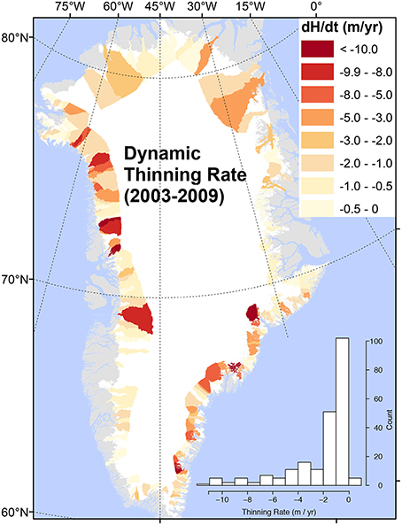
Figure 1. Maximum dynamic thinning rates within each catchment for the period 2003–2009. Shown at lower right is a histogram of the 223 tidewater glaciers with terminus widths greater than 1 km.

2.2. Grounding Line Depth and Glacier Width

This study utilizes the water depth at the grounding line as a measure of the amount of glacial ice exposed to the relatively warm Atlantic Water (AW). Grounding line depths are obtained from both ice penetrating radar and the inversion of airborne gravity measurements. For many glaciers, depth estimates from both radar and gravity inversions are available.

We use the ice base extracted from the Multichannel Coherent Radar Depth Sounder (MCoRDS) ice thickness measurements using both automated and manual techniques (L2 data accessed from https://nsidc.org/data/irmcr2/). The elevation of each ice base is aggregated from all Operation IceBridge (OIB) flights flown from 2009 through 2014. The uncertainty of ice thickness estimates throughout Greenland from the radar instrument is ~10 m (MacGregor et al., 2015), but several nearly-coincident gravity-derived grounding line depths for a single glacier can differ by over 50 m (Boghosian et al., 2015), suggesting substantial across-glacier ice base variability or an increase in radar ranging uncertainty at the grounding line.

Near the terminus of marine-terminating glaciers, radar power attenuates significantly in crevasses, melt water, and through more temperate ice, often preventing the radar from imaging the ice-rock interface. We therefore use gravity-derived bathymetry and sub-ice topography from Boghosian et al. (2015) exclusively for 12 glaciers and to extend radar-derived bathymetry seaward for another 60 glaciers. Using the full suite of geophysical data obtained from NASA OIB program flights between 2009 and 2012, 90 bathymetry models of 54 different fjords were generated by using gravity inversions. These models are available from the National Snow and Ice Data Center (http://nsidc.org/data/docs/daac/icebridge/igbth4/). The base uncertainty in the gravity-derived modeled bathymetry is 50 m (Boghosian et al., 2015). For any glacier with multiple estimates of grounding line depth, we average all estimates from both gravity and radar that are within 200 m across-glacier.

Other constrictions in a fjord such as shallow sills and lateral confinements can reduce the fjord heat flux and subsequently reduce the interaction between ocean and ice. Glacier widths in the linear regressions are from digitized satellite imagery (Howat and Eddy, 2011). Sills are not included in the main analysis as there exists limited evidence that sills significantly shallower than the grounding line are common around Greenland. OIB airborne gravity data rarely extends far enough seaward to reach areas mapped by shipboard echo-sounders (Boghosian et al., 2015). Though we cannot be certain from OIB observations alone whether this apparent lack of shallow sills is true or due to gaps in bathymetry data, the NASA Oceans Melting Greenland (OMG) Earth Ventures project (Fenty et al., 2016) has made significant strides in mapping the continental shelf with a combination of multi-beam echo sonar (MBES) and airborne gravity inversions.

Minimum depths from the combined OIB and OMG data are traced along the deepest pathway between the grounding line and the relatively shallow shelf that extends ~70 km outwards from the coast. We used the International Bathymetric Chart of the Arctic Ocean version 3 (IBCAO3) compilation along with new gravity and swath bathymetry from the NASA OMG mission (https://omg.jpl.nasa.gov/portal/). A continuous map of gravity is used to show the location of the deepest pathways, while depths themselves are taken from OMG swath bathymetry which provides discontinuous coverage across the shelf.

2.3. Using Modeled Ocean State to Estimate Ocean Heat Content

We use ocean model output to estimate the oceanic heat available for melting glaciers for which we have grounding line depths. In situ observations of Greenland's coastal waters are relatively sparse, as fjords are remote and often filled with mélange or sea ice, preventing direct observations. While some of the largest, most accessible fjords have been targeted for oceanographic measurements, short measurement intervals preclude their use in ice sheet-scale change detection studies. Processes governing the large and accessible fjords may not be dominant in other fjords (Straneo et al., 2013).

The ECCO2 project is a specialized branch of the MIT General Circulation Model (MITgcm) developed for Arctic simulations (Nguyen et al., 2011; Rignot et al., 2012). While sparse bathymetry data and the small width of fjords preclude their inclusion in global ocean models, several studies have demonstrated the ECCO2 model's utility for large-scale oceanographic studies around Greenland (Nguyen et al., 2012; Rignot et al., 2012; Porter et al., 2014).

We estimate the ocean heat content (OHC) in the fjord by combining seafloor depths and the ECCO2 ocean state near the mouths of the fjords. The heat nearby on the shelf is used here as a proxy for the potential heat available for glacier melt (Figure 2). For each of the 74 glaciers with a known grounding line depth, OHC is calculated using the closest and deepest column of water in the ECCO2 model. This trade-off between a nearby shallow model point and one that is distant yet deep is tuned to ensure model points are representative of water expected in the fjords from large-scale current patterns (Straneo et al., 2012). For glaciers with a shallow grounding line (less than 200 m), appropriate and nearby model cells are always identified due to the shallow bias of ECCO2 over the inner-shelf (Rignot et al., 2012). For glaciers with grounding lines deeper than this, model cells are selected through the minimization of a loss function with inverse-distance weighting and ECCO2 water column depth. Some fjords are forced to only search for candidate ECCO2 cells in specific cardinal directions to ensure basin continuity. An implicit assumption of this method is water mass homogeneity between the water in the fjord and on the proximal shelf. This similarity between fjord and shelf water is maintained by frequent renewal via buoyancy-driven and intermediary circulation (Straneo and Cenedese, 2015; Jackson et al., 2014) in fjords lacking sills shallower than the pycnocline (~150 m). In the absence of evidence for shallow sills around Greenland, we necessarily apply this assumption of homogeneity for all glaciers in this study.

FIGURE 2

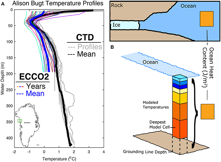
Figure 2. (A) Temperature profiles from both the ECCO2 model and a SeaBird SBE19 CTD for Alison Bugt (74.5828N, −57.0920E). ECCO2 model annual mean temperatures for years 1993–2009 (colored) with climatology in blue. CTD temperature profiles from July 2014, located along the fjord centerline between 18 and 45 km from the glacier terminus, are shown in gray (mean in black). (B) Schematic illustrating the calculation of ocean heat content. For each glacier, an ocean model column is chosen considering both horizontal distance and maximum water depth. OHC is the vertical integral of the difference between each layer's in situ temperature and the freezing point of seawater at that depth.

Ocean heat content is estimated following Martinson and McKee (2012) as:

$\begin{array}{rc}OHC={\displaystyle {\int }_H^{pwd}}\rho c_p\left[T(z)-T_f\right]dz& (1)\end{array}$

where OHC is ocean heat content in J m⁻², pwd is the top of the AW (i.e., the pycnocline), H is the water depth at the grounding line, ρ is the modeled seawater density, c_p is the specific heat capacity of seawater, T is the in situ temperature and T_f is the local freezing point of seawater in °C, and z is the depth of each integration layer. If the nearest ocean model point is shallower than the grounding line depth, the column is assumed isothermal from the seafloor to the deepest model layer (Figure 2).

OHC is calculated using modeled monthly mean temperature, pressure, and salinity from the cube92 version of the ECCO2 model, an observationally-constrained coupled sea ice-ocean-atmosphere model with 50 levels in the vertical and a nominal horizontal resolution of 18 km around Greenland. Monthly heat content estimates are further averaged into both annual and summertime-only means for the period 1993–2009. A comparison of simulated shelf water with ship-based observations near Alison Glacier in northwest Greenland is shown in Figure 2. The model simulates the depth and properties of shelf water with reasonable skill, but is often ≥1°C too cold below the pycnocline. This cold-bias in AW leads to an underestimation of OHC for Alison Glacier, likely a similar bias for any fjord with model bathymetry that is too shallow (Rignot et al., 2012). We calculate a range of ECCO2 OHC estimates for each site by varying the seafloor depth by the Boghosian et al. (2015) uncertainties. The same ECCO2 grid cell may be chosen for nearby glaciers (e.g., Tracy and Heilprin Glaciers in the Thule region), highlighting our assumption of similar far-field ocean forcing being modulated by local-scale factors.

3. Methods

3.1. Spatial Statistics

Spatial autocorrelation describes the propensity for geographically-close observations to co-vary. These spatial statistics are used here to provide insight into the degree of global variability, or spatial randomness of glacier change.

The first step in our spatial analysis is the construction of a spatial weights matrix that adequately captures the strength of connection between nearby observations of glacier thinning rates. Of the several methods that exist for determining the weights matrix for spatial data (Earnest et al., 2007), we use the inverse-distance threshold, where closer observations are weighted more strongly up until a pre-defined limit. The threshold distance used here is the distance which maximizes the global spatial autocorrelation, ~190 km (Figure S1). This criteria also ensures that even the most remote glacier (i.e., Humboldt Glacier in the North) has a minimum of four neighbors. Glaciers in Southeast Greenland have over 30 neighbors using this method. Other methods such as k-nearest neighbors sets the number of observations in each group regardless of spatial distribution. We argue that preserving similar geographical reach supersedes having a consistent number of neighbors for each glacier since thinning is mostly caused by external forcings which varies on a spatial scale.

Secondly, to gain insight into the spatial autocorrelation of glacier thinning we employ the LISA (Local Indicators of Spatial Association) framework. A primary objective of the LISA framework is that each observation gives an indication of the extent of significant spatial clustering of similar values around that observation. The LISA metric used here is the Local Moran's I, a statistic following the two operational objectives of localized spatial autocorrelation method laid out by Anselin (1995, p. 94). The Local Moran's I statistic is calculated as:

$\begin{array}{rc}{I}_i=z_i{\displaystyle \sum _j^{}}{w}_{ij}{z}_j& (2)\end{array}$

where z_i and z_j are standardized observations (mean of 0 and variance of 1), and w_ij are the weights for all locations contained in the defined neighborhood. The Local Moran's I_i is a measure of the spatial autocorrelation estimated for each individual glacier (i.e., the dynamic thinning rates at point i is highly correlated with local neighborhood thinning rates).

The LISA method quantifies correlated (“clustered”) and anti-correlated (“outliers”) glacier change as well as regions with no correlated change (i.e., a high degree of local spatial variability). Clustering indicates that a significant portion of a glacier's variability is shared by neighboring glaciers. The statistical significance of the Local Moran's I can be calculated through a randomization procedure similar to Monte Carlo experiments, using the spatial software package GeoDa (Anselin, 1995). We choose a cut-off for significance as a p < 0.01 after 99,999 spatial autocorrelation permutations using randomized glacier subsets. A glacier having a significant positive Local Moran's I suggests a cluster of similar behavior and therefore spatially coherent change. A grouping of similar Local I values indicates a dominant regional forcing mechanism, such as a change in the oceanic or atmospheric systems.

The LISA method can also classify glaciers as spatial outliers, where an individual catchment is changing differently from other glaciers in its neighborhood. Glaciers in this category have a significant negative Local Moran's I. We interpret these outliers as glaciers with significant localized controls of regional-scale forcing.

We also calculate the Global Moran's I statistic (Ranta et al., 1997) as a metric of the total degree of spatial autocorrelation of all Greenland glacier change. This Global Moran's I quantifies the degree of independence between observations and is proportional to the sum of LISAs for all observations. It is also the slope of the best-fit line when each glacier's neighborhood mean thinning rate is plotted against its own thinning rate. An I value is +1 when similar thinning rates cluster together perfectly and is −1 when dissimilar rates surround each observation (e.g., the colors on a checkerboard). I is 0 for data that are statistically random.

3.2. Exploring Forcing Mechanisms Through Linear Regression

After the quantification of spatial variability and the identification of either regional coherence or local variability, we employ regression analysis to investigate the role of one possible pathway leading to dynamic thinning; deeper grounding line depths and increased fjord heat as potential explanations of the observed patterns of change near the terminus.

The primary driver of change for glaciers in spatially-correlated groupings is likely some large-scale, regional forcing. For outliers and regions without significant clustering, we conjecture that local controls or internal mechanisms exert a large control on any regional forcing. Local controls fall into two categories; those related to internal dynamics of the ice itself (e.g., surge-type glaciers, glacier geometry) and those that modify external forcings (e.g., fjord geometry). For example, Porter et al. (2014) found that deep-grounded marine glaciers are more sensitive to change than those with shallow grounding lines. For the glaciers that do not belong to any cluster, local controls such as fjord geometry must be important and may be significant predictors of glacier change.

In addition to a global regression using all Greenland glaciers with a known grounding line depth, we also do a targeted regional analysis, separating glaciers according to the spatial clusters identified by the Local Moran's I. Climatic differences between the various regions around Greenland's long coastline are significant; from the cold, sea-ice dominated North to the stormy Southeast, with AW temperatures ranging from below 0.5°C to as warm as 8°C, respectively (Straneo et al., 2012). The aggregation of glaciers into these discrete regions is guided by both the Local Moran's I categories and ocean circulation patterns. Three groupings of models have been developed using: (1) the full set of tidewater glaciers, (2) regional subsets, and (3) the full set of tidewater glaciers but excluding those in a given region. A selection of these targeted ordinary least squares (OLS) regression models are presented in detail.

Outliers can exert disproportionate control over OLS regressions, and especially in models with few observations. Most regional models have fewer than a dozen glaciers and so may be particularly susceptible to influence by outliers. The ordinary nonparametric bootstrap method re-samples subsets of each population to quantify the effect of outliers on each model in a Monte-Carlo like approach. We chose a 95% bootstrap confidence interval for each R² based on 1000 iterations.

4. Results

4.1. Spatial Autocorrelation of Dynamic Thinning Rates

For 2003–2009 dynamic thinning rates, the Global Moran's I (the slope of the best-fit line of the scatterplot of each glacier's standardized thinning rate vs. its mean neighborhood thinning rate) is 0.18 (Figure 3B). This I value implies that 18% of the dynamic thinning signal is spatially correlated and that a majority of the observed change of Greenland's marine-terminating glaciers between 2003 and 2009 is spatially uncorrelated. This quantitative approach to estimating the degree of spatial variability in glacier thinning in Greenland confirms previous qualitative assessments (Howat and Eddy, 2011; Csatho et al., 2014; Moon et al., 2014).

FIGURE 3

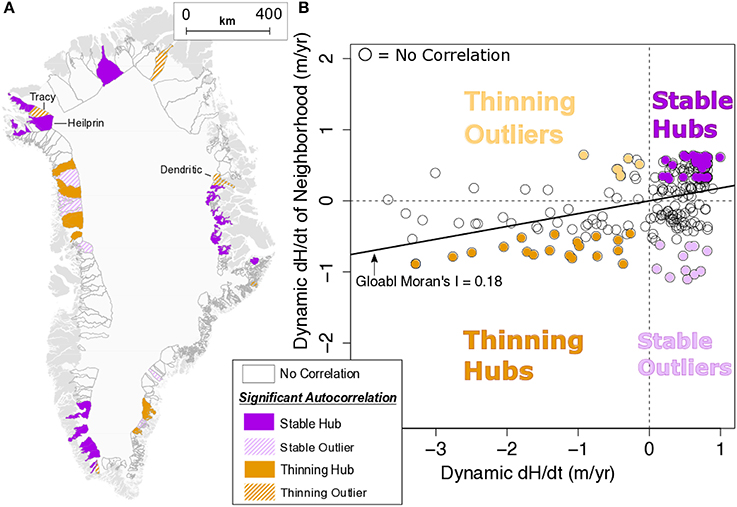
Figure 3. (A) Glacier catchments with significant spatial autocorrelation from the LISA technique based on dynamic thinning rates from 2003 to 2009 (shown in Figure 1). Categories include hubs (solid) and outliers (striped) of both thinning and stable glaciers. Empty catchments show no significant spatial correlation. (B) Global Moran's I scatterplot; standardized dynamic thinning rates for each glacier vs. their neighborhood's weighted-mean thinning rate. Colors are the same as catchments in (A).

The LISA technique identifies patterns of spatial autocorrelation at the glacier scale by categorizing each catchment into one of three groupings; (1) clusters of coherent glacier change, (2) outliers within regional clusters, and (3) glaciers that are not spatially autocorrelated (Anselin, 1995). Glaciers in the first category, which are centers of correlated change, contribute to the Global Moran's I of 0.18. Glaciers in the remaining LISA categories exhibit little or even anti-correlation with neighboring glaciers.

The majority of Greenland's 223 largest glaciers classified by the LISA technique have no significant spatial autocorrelation and exhibit high glacier-to-glacier variability. One hundred and forty-four marine-terminating glaciers fall into this category (Figure 3A). The dynamic thinning of these glaciers share no statistical relationship to nearby glaciers, from which we infer that regional forcing of these glaciers must be modulated by local, glacier-scale controls (Csatho et al., 2014; Moon et al., 2014). Single centers of spatial correlation also exist (e.g., Ryder in the north) but are less representative of a robust regional pattern as their neighbors are not themselves centers of coherence.

Several regions of coherent dynamic thinning are identified by the LISA analysis (Figure 3A). The Southwest, Thule, and Scoresby Sund all contain numerous glaciers that are identified as cluster centers. Because dynamic thinning in all of these regions is relatively small, this clustering is evidence of a lack of uniform large-scale change. In total there are 39 glaciers included in the LISA category of correlated stability and another 20 are centers of correlated thinning (Figure 3A).

The LISA technique also identifies 20 outliers, where the change of an individual glacier change is opposite that of neighboring glaciers (i.e., anti-correlated). Tracy and Dendritic glaciers in the Thule and Scoresby Sund regions, respectively, are identified as examples of these outlying glaciers (Figure 3A). Within their regions, which are dominated by stability, these glaciers are thinning significantly. This spatial statistical approach is consistent with the identification of Tracy as an outlier in the Thule region by Porter et al. (2014). They posited that Tracy is likely more sensitive to ocean forcing than its neighboring glacier, Heilprin, due to a difference in the area of ice exposed to deep and warm AW.

4.2. Regression Analysis

The results from the LISA analysis reveal that most regions around Greenland either (a) contain outliers or (b) lack any significant spatial correlation (i.e., exhibit high spatial variability). The findings of Porter et al. (2014) suggest that the water depth at the grounding line (a glacier-scale control that varies greatly from fjord to fjord) could be an important explanatory variable in OLS regressions. We investigate one of the potential drivers of this regionally-varying signal by constructing OLS models with grounding line depths and modeled OHC as independent variables, regressed against the maximum dynamic thinning rate within each glacier catchment (Figure 4).

FIGURE 4

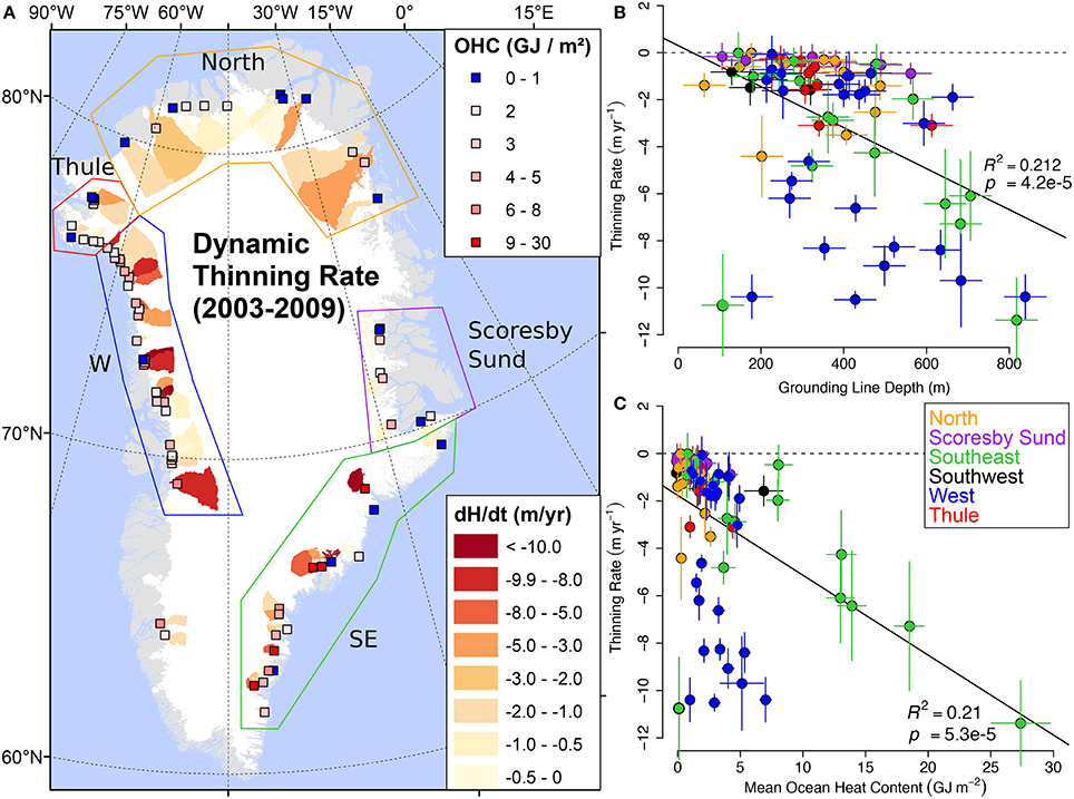
Figure 4. (A) Dynamic thinning rates (2003–2009) for all 74 glaciers with known grounding line depths are shown in Figure 1 along with OHC from ECCO2 model (colored boxes). OLS regression results for annualized dynamic thinning rates (m yr⁻¹) with (B) grounding line depths (m) and (C) mean OHC (GJ m⁻²) for all 74 tidewater glaciers. Also indicated is the global coefficient of determination. Regional regression groupings are annotated.

The dependent variable (the catchment-maximum dynamic thinning rate) is compared to two predictive variables: the water depth at the grounding line and the modeled mean OHC. For all 74 glaciers with known grounding line depths, the relationship between grounding line and thinning rate is modest, yet statistically significant, with a regression slope line of −0.0087 and an R² of 0.212 ± 0.12 and p of 4.2 × 10⁻⁵. One interpretation of this slope is that an extra 87 m of water depth at terminus is roughly equivalent to 1 m yr⁻¹ dynamic thinning. Two glaciers, Midgaard in the southeast and Upernavik NW in the northwest, have anomalously shallow grounding line depths for their maximum dynamic thinning rates (annotated in Figures 5, 7, respectively). For Midgaard, the grounding line depth estimate is obtained from a gravity-inversion with topography constraints from Helheim Glacier, over 70 km away (Boghosian et al., 2015). Inspection of more recent radargrams from Midgaard show bed horizons up to 300 m lower than predicted in Boghosian et al. (2015). This discrepancy suggests a significant horizontal density gradient between Helheim and Midgaard Glaciers that increases the uncertainty in the grounding line depth estimates obtained from gravity-inversions (Boghosian et al., 2015). Upernavik NW is a small glacier that was, until recently, a tributary of the main Upernavik N glacier, and may have temporarily high dynamic thinning rates unrelated to changes in ocean forcing (Khan et al., 2013).

FIGURE 5

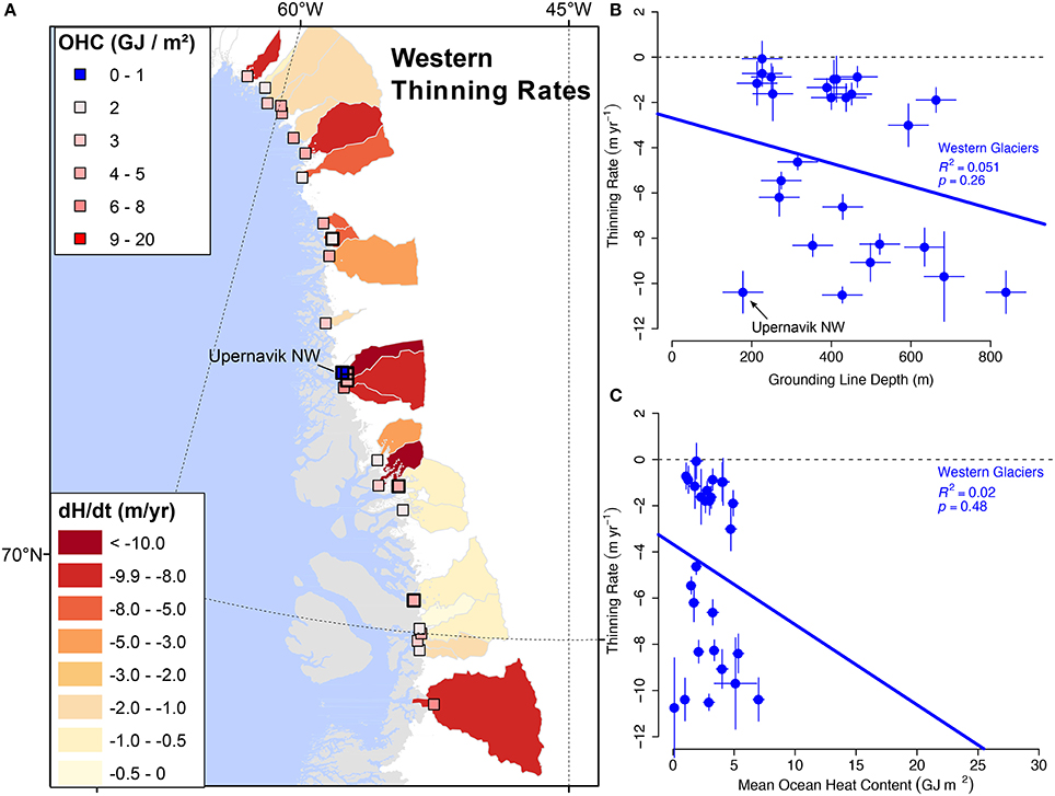
Figure 5. (A) Annualized dynamic thinning rates (dH/dt) and modeled OHC for the period 2003–2009 for Western tidewater glaciers. (B) OLS regression of grounding line depth (m) with the maximum dynamic thinning rate for each catchment (m yr⁻¹). Scatterplot shows Western glaciers as blue points. Same for (C) except with ocean heat content (OHC) in GJ m⁻² as the independent variable. The coefficient of determination R² shown for Western glaciers.

Beyond the modest correlation between grounding line depth and glacier dynamic thinning rate, the influence of warm water availability is explored using modeled OHC from ECCO2. In general, ocean heat content is higher in fjords with deeper grounded glaciers, but the relationship between OHC and grounding line depth is not linear because of regional variability in the ocean thermal structure. Regression models that incorporate ocean thermal state in the form of estimates of OHC (Figure 4C) are not improved (R² = 0.206 ± 0.10, p = 5.3 × 10⁻⁵).

Visual inspection of Figures 4B,C shows three distinct populations of glaciers. Broadly, these are (1) glaciers with small thinning rates and low OHC, (2) glaciers that thin as OHC increases, and (3) glaciers with the full range of thinning rates with a relatively low OHC (e.g., less than ~7 GJ m⁻²). This last set of glaciers are nearly entirely contained within the Western Region. The single exception to this geographic grouping is Midgaard Glacier of the Southeast Region.

To help understand the scattered appearance of the All Glacier regression shown in Figure 4, we separate each region into their own OLS regression model. In addition to those discussed in the following Regression Analysis sections, results from the remaining regions (i.e., the North, Thule, and Scoresby Sund regions) are presented and discussed in the Supplementary Material.

Regional Regressions: Western Greenland

We construct regional OLS models using both grounding line depth and OHC for Western glaciers (Figure 5A). There is little correlation between dynamic thinning rate and either grounding line depth or OHC in this region (Figures 5B,C). The R² for grounding line depth and thinning rate of 0.05 is insignificant (p = 0.26). The inclusion of the ocean thermal state through OHC does not improve the OLS model for these glaciers (R² = 0.02). These results indicate that although the West coast is thinning at a high rate as a whole (Csatho et al., 2014), there is no relationship between patterns of ocean heat and individual glacier change. The poor correlation with grounding line depth in this region is primarily a result of thinning rates that fall into two groups, above and below ~4 m yr⁻¹. There is little difference in the range of grounding line depths between these high and low thinning rate groups (Figure 5B). For example, some glaciers in the northern section of this region, such as Kong Oscar, have deep grounding lines but comparatively low dynamic thinning rates (Csatho et al., 2014). Incorporating ocean state estimates from the ECCO2 model does not improve the relationship (Figure 5C).

Regression models that include all glaciers except those in Western Greenland (Figures 6A,B) reveal a clear connection between dynamic thinning and both grounding line depth (R² = 0.47 ± 0.14) and OHC (R² = 0.74 ± 0.15). For this group of glaciers, including the ocean state does improve the correlation with dynamic thinning rate; ~74% of the variance in dynamic thinning rate of these marine-terminating glaciers can be explained by modeled mean OHC from nearby on the shelf.

FIGURE 6

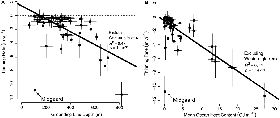
Figure 6. (A) OLS regression of grounding line depth (m) with the maximum dynamic thinning rate for each catchment (m yr⁻¹) for all glaciers except those in Western Greenland (as shown in Figure 5C). Panel (B) shows ocean heat content (OHC) in GJ m⁻² as the independent variable. The coefficient of determination R² shown for all remaining glaciers.

Regional Regressions: Southeast

With the exception of Midgaard, glaciers located on Greenland's East coast lie closest to the line-of-best-fit for both regression models that use the full glacier set (Figure 4). Glaciers with the most pronounced relationship between dynamic thinning rate and grounding line depth (i.e., those that fall very close to the line-of-best-fit) are in the Southeast and plotted separately in Figure 7. The OLS models for the Southeast region, with 15 glaciers, has a coefficient of determination of 0.71 ± 0.16 with a slope of 0.013. The relationship between ocean heat and glacier thinning is also strongest in the Southeast, with an R²=0.83 ± 0.15 and a slope of −38.1. Southeastern glaciers are more sensitive to grounding line depth and OHC than any other region. Subsurface AW in this region, the warmest in all of Greenland (Straneo et al., 2012), is likely the cause for this high correlation.

FIGURE 7

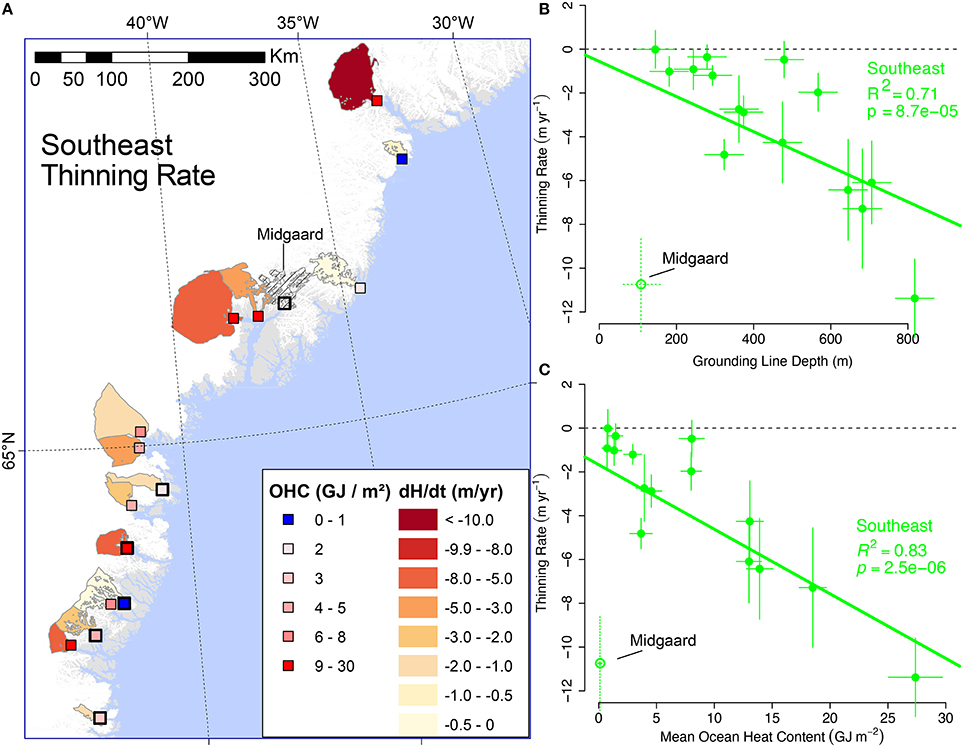
Figure 7. As in Figure 5: (A) annual dynamic thinning rates (m yr⁻¹) and modeled mean ocean heat content for the period 2003–2009, but instead for Southeast tidewater glaciers. (B) OLS regression of grounding line depth (m) with the maximum dynamic thinning rate for each catchment (m yr⁻¹). Scatterplot shows Southeast glaciers as green points. Same for (C) except with ocean heat content (OHC) as the independent variable. The coefficient of determination is shown for Southeast glaciers.

Midgaard Glacier clearly departs from the relationship between dynamic thinning and grounding line depth. As mentioned earlier, there is larger uncertainty in the gravity-derived grounding line depth of Midgaard Glacier. However, this increased uncertainty in seafloor depths (and therefore also OHC) is alone unlikely to fully account for Midgaard's apparent shallow and cold fjord Figures 7B,C. Errors in thinning rates can at most account for ± 3 m yr⁻¹ (Csatho et al., 2014) of surface elevation change. Alternatively, we can consider Midgaard as a true outlier; a glacier that is thinning at a rate comparable to nearby Kangerlussuaq and Helheim Glaciers but grounded in water only ~100 m deep. Given that the thermocline lies below this depth on the east coast (Straneo et al., 2012), there is little ocean heat available to melt the ice face, suggesting an alternative mechanism for Midgaard.

Accounting for Glacier Width and Sills

Two other major aspects of fjord geometry that could modulate ice-ocean interactions are the width of the fjord near the terminus (Seale et al., 2011; Carr et al., 2014) and the presence of sills. For glaciers terminating in wide fjords (≥~5 km), across-fjord hydrographic variability becomes more important due to the influence of Earth's rotation. In this way, any changes in ocean forcing on the continental shelf will be more easily transmitted toward the glacier front in wider fjords. In addition to affecting ice front ablation, wide termini can be more sensitive to change due to reduced sidewall buttressing. However, we find here that glacier width has no correlation with dynamic thinning rate for Greenland's marine-terminating glaciers (Figure 8A). In general, the widest glaciers are in the north where dynamic thinning is relatively low (e.g., Humboldt Glacier).

FIGURE 8

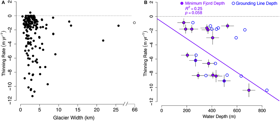
Figure 8. (A) Scatterplot of glacier width vs. maximum dynamic thinning rate (m yr⁻¹) for the total glacier set. Humboldt glacier has a width of over 66 km (outside the bounds of the plot) and is indicated as an open circle. (B) OLS regression for Northwest glaciers, as in Figure 5, instead for the minimum seafloor depths (m) along trough centerlines from the head of the fjord to the outer shelf using NASA OMG swath bathymetry and airborne gravity data. Grounding line depths (used in original analysis) are in open blue circles, minimum fjord depths for those glaciers are in solid purple.

Although very few sills were identified using the OIB gravity data (Boghosian et al., 2015), flight coverage down-fjord is not comprehensive and cannot rule out the presence of bathymetric constrictions. In Northwest Greenland, where the lack of correlation between OHC and glacier change is most stark, OMG has recently mapped many fjords and glacial troughs (Fenty et al., 2016), enabling the inclusion of sills and banks into a regional regression model. A total of 18 glaciers in the Northwest region are found to have local minima that are shallower than their grounding lines (Figure 8B). The average adjustment for these bathymetric minima is 66 m upward with some sills 200 m shallower than at the grounding line.

The Northwest Glaciers OLS regression model with minimum water depths shows an improved fit compared with the original regional regression with grounding line depths alone (Figure 5B). The modest increase in R² to 0.25 (p = 0.058) is a result of relatively larger sills in the more stable glaciers (less than 3 m yr⁻¹). For this population of six glaciers, all bathymetric troughs have shallower seafloor features than their grounding lines. These constrictions could act as additional barriers to the heat flux toward the ice face and possibly be responsible for the reduced thinning rates of this population (Straneo and Cenedese, 2015). Glaciers with higher thinning rates are also often shallower elsewhere along their lowest pathway across the shelf than at the grounding line, but by a smaller degree. There is no obvious geographical relationship (e.g., a latitudinal dependency) in the difference between grounding line depth and sill height.

5. Discussion

Possible explanations for the lack of correlation between grounding line depth and OHC with glacier change in the West include (1) OHC on the shelf may not be a good proxy for heat reaching the glacier termini in this region, (2) grounding line depth and/or ocean heat are not predictive of glacier change here, or (3) inadequate bathymetric data or inadequate observational constraints results in significant ocean model deficiencies along this stretch of Greenland's coast. The response timescale of glacier melt to ocean warming is poorly understood, leaving open the possibility that changes during the ICESat record are not adequately captured by the time period chosen for ECCO2 OHC estimates. Also, ECCO2 output are averaged over a period that predates ICESat by more than a decade, possibly underestimating OHC compared with the more recent period (Rignot et al., 2012). Besides grounding lines depth and OHC, other factors could have contributed more to glacier thinning variability in the West region. In addition to the thermal effects of liquid water at the ice-ocean interface, turbulence plays an important role in the efficiency of heat delivery to the ice (Straneo et al., 2016). This means that fjord current velocities and subglacial discharge rates, neither of which are expected to be uniform across this region, could be responsible for the observed thinning patterns.

One possibility is that any causal link between grounding line depth and dynamic glacier thinning in Western Greenland is quashed by other drivers of change. Additionally, a lagged response between ocean warming and dynamic thinning could also play a role, particularly in shallow-sill fjords characterized by episodic flushes between quiescent periods (Gladish et al., 2015). Large differences in the thermal structure of fjords between the ocean model and in situ hydrographic observations provides some evidence for shortcomings associated with the model solutions on the West coast. For Jakobshavn Isbrae (Gladish et al., 2015), Upernavik glaciers (Straneo et al., 2012), and near Alison Glacier (Figure 2A), a comparison of model annual means and CTD observations show that ECCO2 output underestimates AW temperatures near these fjord. This ECCO2 cold bias, combined with our assumption of an isothermal state below the deepest model level and the pressure dependency of the freezing point of seawater, likely leads to an underestimation of OHC, exacerbated for deeper glaciers.

The absence of strong correlations in many regions points toward the importance of glacier dynamics in controlling the patterns of variability in dynamic thinning identified by the LISA analysis. This reinforces (Gladish et al., 2015), who found it difficult to explain annual patterns of retreat of Jakobshavn Glacier with fjord water properties alone. Just as fjord geometry modulates ocean heat flux toward ice sheets, glacier geometry imparts a first-order control on perturbations at the terminus (Nick et al., 2009). In this way, geometry and internal dynamics can determine a glaciers response long after the initial change in forcing. In this way, glacier geometry would be a confounder in the regression analysis by influencing both grounding line depth and dynamic glacier thinning. Apart from the difficulty of capturing the geometric control on internal glacier dynamics with any single metric, confounding precludes its inclusion in the statistical approach used in this paper.

6. Conclusions

The regional patterns identified by the LISA analysis suggests that there are significant local, glacier-scale controls on the rates of glacier change in Greenland. The Thule, Scoresby Sund, and Southwest regions are consistently stable but with at least one outlying glacier that is thinning. The Northwest and Southeast regions are thinning overall but with several stable outliers, while the remaining glaciers show no spatial autocorrelation. For dynamic thinning rates, changes at the terminus, such as frontal ablation, will dominate any observed signal. We explore the relationship of termini forcing and glacier change by building OLS regression models for grounding line depth and fjord heat, previous identified as a driver of glacier melt in both models and in observations of individual fjords. We extend this analysis to 74 marine-terminating glaciers around Greenland and find that the co-variability of ocean heat content and dynamic thinning rate is highest in the Southeast and Scoreby Sund regions, though insignificant in Western glaciers.

Overall, dynamic thinning of Greenland's marine-terminating glaciers exhibit a high degree of spatial variability. Across 223 of Greenland's largest tidewater glaciers, only ~18% of the dynamic thinning rate is spatially correlated. Some regions exhibit spatially-coherent thinning, while those regions with little or no dynamic thinning exhibit spatially correlated behavior. Conversely, in regions undergoing widespread thinning, the patterns of glacier change develop in a spatially variable way, varying from glacier to glacier.

The local-scale variability in ocean heat content (estimated by combining grounding line depths and ocean model output) explains more of the variability in dynamic thinning rate than water depth alone. For all glaciers except those on the West coast, modeled OHC explains ~74% ± 0.15 of the variability in glacier thinning. This correlation increases to ~83% ± 0.15 for just Southeast glaciers, implying that deeply grounded termini in this region are most sensitive to ocean forcing.

Glaciers in the West are thinning from dynamic processes (Csatho et al., 2014), yet there is little correlation with grounding line depth and none with modeled ocean heat content. This lack of correlation is either a real phenomenon or possibly caused by ocean model deficiencies in this region. Regression models that include sill and bank heights are an improvement over grounding line depth alone, suggesting that all aspects of fjord geometry should be considered in assessing the sensitivity of a glacier to ocean forcing.

The spatial relationships revealed here have implications for research planning and trend extrapolation. Glaciers identified as outliers using either the LISA technique or OLS regression should be targeted for process based studies to better understand their driving processes. However, these same outliers should not be used individually to infer future ice sheet change. Conversely, glaciers identified as hubs of change represent regional coherence and therefore better targets for long-term monitoring.

Author Contributions

All authors contributed to the text. KT and AB were responsible for the gravity inversions and inclusion of OMG bathymetry. DP handled much of the statistical analysis. BC processed the dynamic thinning rate estimates.

Funding

This work was supported by NASA grants NNX12AB70G and NNX13AD25A.

Conflict of Interest Statement

The authors declare that the research was conducted in the absence of any commercial or financial relationships that could be construed as a potential conflict of interest.

Acknowledgments

We thank Ian Fenty and Dimitris Menemenlis for providing the ECCO2 model output. We thank the Associate Editor Alun Hubbard and two reviewers, including Martin Truffer, for greatly improving this paper.

Supplementary material

The Supplementary Material for this article can be found online at: https://www.frontiersin.org/articles/10.3389/feart.2018.00090/full#supplementary-material

References

Amundson, J. M., Fahnestock, M., Truffer, M., Brown, J., Lüthi, M. P., and Motyka, R. J. (2010). Ice mélange dynamics and implications for terminus stability, Jakobshavn Isbræ, Greenland. J. Geophys. Res. 115:F01005. doi: 10.1029/2009JF001405

CrossRef Full Text | Google Scholar

Anselin, L. (1995). Local indicators of spatial association—LISA. Geograph. Anal. 27, 93–115.

Google Scholar

Boghosian, A., Tinto, K., Cochran, J. R., Porter, D., Elieff, S., Burton, B. L., et al. (2015). Resolving bathymetry from airborne gravity along Greenland fjords. J. Geophys. Res. Solid Earth 120, 8516–8533. doi: 10.1002/2015JB012129

CrossRef Full Text | Google Scholar

Carr, J. R., Stokes, C., and Vieli, A. (2014). Recent retreat of major outlet glaciers on Novaya Zemlya, Russian Arctic, influenced by fjord geometry and sea-ice conditions. J. Glaciol. 60, 155–170. doi: 10.3189/2014JoG13J122

CrossRef Full Text | Google Scholar

Cook, S., Rutt, I. C., Murray, T., Luckman, A., Zwinger, T., Selmes, N., et al. (2014). Modelling environmental influences on calving at Helheim Glacier in eastern Greenland. Cryosphere 8, 827–841. doi: 10.5194/tc-8-827-2014

CrossRef Full Text | Google Scholar

Csatho, B. M., Schenk, A. F., van der Veen, C. J., Babonis, G., Duncan, K., Rezvanbehbahani, S., et al. (2014). Laser altimetry reveals complex pattern of Greenland Ice Sheet dynamics. Proc. Natl. Acad. Sci. U.S.A. 111, 18478–18483. doi: 10.1073/pnas.1411680112

PubMed Abstract | CrossRef Full Text | Google Scholar

Earnest, A., Morgan, G., Mengersen, K., Ryan, L., Summerhayes, R., and Beard, J. (2007). Evaluating the effect of neighbourhood weight matrices on smoothing properties of Conditional Autoregressive (CAR) models. Int. J. Health Geograph. 6:54. doi: 10.1186/1476-072X-6-54

PubMed Abstract | CrossRef Full Text | Google Scholar

Enderlin, E. M., Howat, I. M., and Vieli, A. (2013). High sensitivity of tidewater outlet glacier dynamics to shape. Cryosphere 7, 1007–1015. doi: 10.5194/tc-7-1007-2013

CrossRef Full Text | Google Scholar

Fenty, I., Willis, J., Khazendar, A., Dinardo, S., Forsberg, R., Fukumori, I., et al. (2016). Oceans melting Greenland: early results from NASA's ocean-ice mission in Greenland. Oceanography 29, 72–83. doi: 10.5670/oceanog.2016.100

CrossRef Full Text | Google Scholar

Giebultowicz, S., Ali, M., Yunus, M., and Emch, M. (2011). A comparison of spatial and social clustering of cholera in Matlab, Bangladesh. Health Place 17, 490–497. doi: 10.1016/j.healthplace.2010.12.004

PubMed Abstract | CrossRef Full Text | Google Scholar

Gladish, C. V., Holland, D. M., Rosing-Asvid, A., Behrens, J. W., and Boje, J. (2015). Oceanic boundary conditions for Jakobshavn Glacier. Part I: variability and renewal of ilulissat icefjord waters, 2001–14. J. Phys. Oceanogr. 45, 3–32. doi: 10.1175/JPO-D-14-0044.1

CrossRef Full Text | Google Scholar

Howat, I. M., and Eddy, A. (2011). Multi-decadal retreat of Greenland's marine-terminating glaciers. J. Glaciol. 57, 389–396. doi: 10.3189/002214311796905631

CrossRef Full Text | Google Scholar

Howat, I. M., Joughin, I., and Scambos, T. A. (2007). Rapid changes in ice discharge from Greenland outlet glaciers. Science 315, 1559–1561. doi: 10.1126/science.1138478

PubMed Abstract | CrossRef Full Text | Google Scholar

Howat, I. M., Negrete, A., and Smith, B. E. (2014). The Greenland Ice Mapping Project (GIMP) land classification and surface elevation data sets. Cryosphere 8, 1509–1518. doi: 10.5194/tc-8-1509-2014

CrossRef Full Text | Google Scholar

Jackson, R. H., Straneo, F., and Sutherland, D. A. (2014). Externally forced fluctuations in ocean temperature at Greenland glaciers in non-summer months. Nat. Geosci. 7, 503–508. doi: 10.1038/NGEO2186

CrossRef Full Text | Google Scholar

Khan, S. A., Kjær, K. H., Korsgaard, N. J., Wahr, J., Joughin, I. R., Timm, L. H., et al. (2013). Recurring dynamically induced thinning during 1985 to 2010 on Upernavik Isstrøm, West Greenland. J. Geophys. Res. Earth Surf. 118, 111–121. doi: 10.1029/2012JF002481

CrossRef Full Text | Google Scholar

MacGregor, J. A., Fahnestock, M. A., Catania, G. A., Paden, J. D., Gogineni, S. P., Young, S. K., et al. (2015). Radiostratigraphy and age structure of the Greenland Ice Sheet. J. Geophys. Res. Earth Surf. 120, 212–241. doi: 10.1002/2014JF003215

PubMed Abstract | CrossRef Full Text | Google Scholar

Martinson, D. G., and McKee, D. C. (2012). Transport of warm Upper Circumpolar Deep Water onto the western Antarctic Peninsula continental shelf. Ocean Sci. 8, 433–442. doi: 10.5194/os-8-433-2012

CrossRef Full Text | Google Scholar

McFadden, E. M., Howat, I. M., Joughin, I., Smith, B. E., and Ahn, Y. (2011). Changes in the dynamics of marine terminating outlet glaciers in west Greenland (2000-2009). J. Geophys. Res. 116:F02022. doi: 10.1029/2010JF001757

CrossRef Full Text | Google Scholar

Moon, T., Joughin, I., Smith, B., van den Broeke, M. R., van de Berg, J., Noël, B., et al. (2014). Distinct patterns of seasonal Greenland glacier velocity. Geophys. Res. Lett. 41, 7209–7216. doi: 10.1002/2014GL061836

PubMed Abstract | CrossRef Full Text | Google Scholar

Moon, T., Joughin, I., Smith, B. E., and Howat, I. (2012). 21st-century evolution of Greenland outlet glacier velocities. Science 336, 576–578. doi: 10.1126/science.1219985

PubMed Abstract | CrossRef Full Text | Google Scholar

Mueller, G. S., Clayton, A. L., Zahnd, W. E., Hollenbeck, K. M., Barrow, M. E., Jenkins, W. D., et al. (2015). Geospatial analysis of Cancer risk and residential proximity to coal mines in Illinois. Ecotoxicol. Environ. Saf. 120, 155–162. doi: 10.1016/j.ecoenv.2015.05.037

PubMed Abstract | CrossRef Full Text | Google Scholar

Murray, T., Scharrer, K., James, T. D., Dye, S. R., Hanna, E., Booth, A. D., et al. (2010). Ocean regulation hypothesis for glacier dynamics in southeast Greenland and implications for ice sheet mass changes. J. Geophys. Res. Earth Surf. 115:F03026. doi: 10.1029/2009JF001522

CrossRef Full Text | Google Scholar

Nguyen, A. T., Kwok, R., and Menemenlis, D. (2012). Source and pathway of the Western Arctic Upper Halocline in a data-constrained coupled ocean and sea ice model. J. Phys. Oceanogr. 42, 802–823. doi: 10.1175/JPO-D-11-040.1

CrossRef Full Text | Google Scholar

Nguyen, A. T., Menemenlis, D., and Kwok, R. (2011). Arctic ice-ocean simulation with optimized model parameters: approach and assessment. J. Geophys. Res. 116:C04025. doi: 10.1029/2010JC006573

CrossRef Full Text | Google Scholar

Nick, F. M., Vieli, A., Howat, I. M., and Joughin, I. (2009). Large-scale changes in Greenland outlet glacier dynamics triggered at the terminus. Nat. Geosci. 2, 110–114. doi: 10.1038/ngeo394

CrossRef Full Text | Google Scholar

O'Leary, M., and Christoffersen, P. (2013). Calving on tidewater glaciers amplified by submarine frontal melting. Cryosphere 7, 119–128. doi: 10.5194/tc-7-119-2013

CrossRef Full Text | Google Scholar

Porter, D. F., Tinto, K. J., Boghosian, A., Cochran, J. R., Bell, R. E., Manizade, S. S., et al. (2014). Bathymetric control of tidewater glacier mass loss in northwest Greenland. Earth Planet. Sci. Lett. 401, 40–46. doi: 10.1016/j.epsl.2014.05.058

CrossRef Full Text | Google Scholar

Pritchard, H. D., Arthern, R. J., Vaughan, D. G., and Edwards, L. A. (2009). Extensive dynamic thinning on the margins of the Greenland and Antarctic ice sheets. Nature 461, 971–975. doi: 10.1038/nature08471

PubMed Abstract | CrossRef Full Text | Google Scholar

Ranta, E., Kaitala, V., Lindström, J., and Helle, E. (1997). The moran effect and synchrony in population dynamics. Oikos 78:136. doi: 10.2307/3545809

CrossRef Full Text | Google Scholar

Rignot, E., Fenty, I., Menemenlis, D., and Xu, Y. (2012). Spreading of warm ocean waters around Greenland as a possible cause for glacier acceleration. Ann. Glaciol. 53, 257–266. doi: 10.3189/2012AoG60A136

CrossRef Full Text | Google Scholar

Rignot, E., Fenty, I., Xu, Y., Cai, C., and Kemp, C. (2015). Undercutting of marine-terminating glaciers in West Greenland. Geophys. Res. Lett. 42:5909–5917. doi: 10.1002/2015GL064236

CrossRef Full Text | Google Scholar

Rignot, E., and Kanagaratnam, P. (2006). Changes in the velocity structure of the Greenland ice sheet. Science 311, 986–990. doi: 10.1126/science.1121381

PubMed Abstract | CrossRef Full Text | Google Scholar

Seale, A., Christoffersen, P., Mugford, R. I., and O'Leary, M. (2011). Ocean forcing of the Greenland Ice Sheet: calving fronts and patterns of retreat identified by automatic satellite monitoring of eastern outlet glaciers. J. Geophys. Res. Earth Surf. 116:F03013. doi: 10.1029/2010JF001847

CrossRef Full Text | Google Scholar

Shepherd, A., Hubbard, A., Nienow, P., King, M., McMillan, M., and Joughin, I. (2009). Greenland ice sheet motion coupled with daily melting in late summer. Geophys. Res. Lett. 36:L01501. doi: 10.1029/2008GL035758

CrossRef Full Text | Google Scholar

Shepherd, A. P., Ivins, E. R., A. G. Barletta, V. R., Bentley, M. J., Bettadpur, S., Briggs, K. H., et al. (2012). A reconciled estimate of ice-sheet mass balance. Science 338, 1183–1189. doi: 10.1126/science.1228102

PubMed Abstract | CrossRef Full Text | Google Scholar

Straneo, F., and Cenedese, C. (2015). The dynamics of Greenland's Glacial Fjords and their role in climate. Annu. Rev. Mar. Sci. 7, 89–112.

PubMed Abstract | Google Scholar

Straneo, F., Hamilton, G., Stearns, L., and Sutherland, D. (2016). Connecting the Greenland ice sheet and the ocean: a case study of Helheim Glacier and Sermilik Fjord. Oceanography 29, 34–45. doi: 10.5670/oceanog.2016.97

CrossRef Full Text | Google Scholar

Straneo, F., Heimbach, P., Sergienko, O., Hamilton, G., Catania, G., Griffies, S., et al. (2013). Challenges to understanding the dynamic response of Greenland's marine terminating glaciers to oceanic and atmospheric forcing. Bull. Am. Meteorol. Soc. 94, 1131–1144. doi: 10.1175/BAMS-D-12-00100.1

CrossRef Full Text | Google Scholar

Straneo, F., Sutherland, D. A., Holland, D., Gladish, C., Hamilton, G. S., Johnson, H. L., et al. (2012). Characteristics of ocean waters reaching Greenland's glaciers. Ann. Glaciol. 53, 202–210. doi: 10.3189/2012AoG60A059

CrossRef Full Text | Google Scholar

Sugiyama, S., Skvarca, P., Naito, N., Enomoto, H., Tsutaki, S., Tone, K., et al. (2011). Ice speed of a calving glacier modulated by small fluctuations in basal water pressure. Nat. Geosci. 4, 597–600. doi: 10.1038/NGEO1218

CrossRef Full Text | Google Scholar

Truffer, M., and Motyka, R. J. (2016). Where glaciers meet water: subaqueous melt and its relevance to glaciers in various settings. Rev. Geophys. 54, 220–239. doi: 10.1002/2015RG000494

CrossRef Full Text | Google Scholar

van den Broeke, M., Bamber, J., Ettema, J., Rignot, E., Schrama, E., van de Berg, W. J., et al. (2009). Partitioning recent Greenland mass loss. Science 326, 984–986. doi: 10.1126/science.1178176

PubMed Abstract | CrossRef Full Text | Google Scholar

Walsh, K. M., Howat, I. M., Ahn, Y., and Enderlin, E. M. (2012). Changes in the marine-terminating glaciers of central east Greenland, 2000–2010. Cryosphere 6, 211–220. doi: 10.5194/tc-6-211-2012

CrossRef Full Text | Google Scholar

Xu, Y., Rignot, E., Menemenlis, D., and Koppes, M. (2012). Numerical experiments on subaqueous melting of Greenland tidewater glaciers in response to ocean warming and enhanced subglacial discharge. Ann. Glaciol. 53, 229–234. doi: 10.3189/2012AoG60A139

CrossRef Full Text | Google Scholar