Examining the Geologic Link of Arsenic Contamination in Groundwater in Orange County, North Carolina

Introduction

Arsenic is an extremely pervasive, naturally occurring, and potentially hazardous element that is found in air, soil, water, organisms, and rocks. While arsenic occurs in organic and inorganic forms, inorganic arsenic compounds are far more toxic than organic arsenic compounds (Brown and Ross, 2002). Inorganic arsenic, most commonly found as arsenite (As³⁺) or arsenate (As⁵⁺), is mainly consumed by humans through drinking water (Maascheleyn et al., 1991; Welch et al., 2000; Kim et al., 2011), but can still be consumed if contaminated water is used for food preparation or irrigation (McCarty et al., 2011; World Health Organization, 2016). Sources of inorganic arsenic include natural concentrations in certain minerals and anthropogenic sources from mining, industrial, and agricultural activities (Naujokas et al., 2013; Smedley and Kinniburgh, 2013; Biswas et al., 2016). Excessive and chronic low-level arsenic exposure is associated with numerous negative health effects including, but not limited to death, lung and skin cancer, blackfoot disease, vascular and heart disease, skin problems, diabetes, and many more (Brown and Ross, 2002; Tseng, 2005; Kim et al., 2011; McCarty et al., 2011; Naujokas et al., 2013). The evidence suggesting the toxic effects of arsenic ingestion, even at very low doses (low μg/L range), has given rise to new regulations and guidelines for drinking water quality in many countries. The World Health Organization (WHO) adopted a guideline of 10 μg/L of arsenic in drinking water in 1993. Currently in the United States, arsenic in drinking water is controlled by a US-EPA drinking water standard of 10 μg/L (USEPA, 2001). However, this standard is not enforced by the EPA for private wells in the United States (Private Drinking Water Wells, 2018), so unnoticed arsenic contamination in private wells has the potential to lead to arsenic poisoning.

In recent decades, high concentrations of naturally occurring arsenic in groundwater have been observed globally, including locations in Southeast Asia, South America, and the Western United States, which is of concern due to the potential health effects that people may experience in these places from high arsenic consumption (Nordstrom, 2002; Smedley and Kinniburgh, 2002; McCarty et al., 2011). Bangladesh is widely recognized as the most problematic area because of the high concentrations of arsenic observed in the region and the large population that rely on and use the groundwater there (Nordstrom, 2002; Smedley and Kinniburgh, 2002). In Bangladesh, reducing conditions have lead to the dissolution, desorption, and release of arsenic from metal oxide minerals into groundwater supplies. Concentrations as high as 3,200 μg/L have been observed and the population at risk of excessive arsenic exposure through groundwater is estimated at 57 million (Smedley and Kinniburgh, 2002; Yunus et al., 2016). Arid, oxidizing environments are also associated with groundwater arsenic contamination and problematic areas have been identified in some countries, such as Chile and Argentina. In oxidizing environments, arsenic is primarily released from sulfides and volcanic glass sediments and arsenate is the dominant speciation (Smedley and Kinniburgh, 2002; Nicolli et al., 2012; Murray et al., 2016). In addition to the two main regimes of arsenic mobilization (reducing and oxidizing), arsenic concentrations in groundwater have been found to be higher in closed basins, regions with geothermal water, and in some mining districts where sulfides in tailings have been oxidized and leached arsenic into surface and groundwater (Welch et al., 2000; Smedley and Kinniburgh, 2002; Biswas et al., 2016; Murray et al., 2016). Finding elevated levels of arsenic in these types of environments is typical and an increasing number of regions are reporting arsenic concentration exceedances in groundwater as testing and monitoring becomes more ubiquitous.

The Piedmont region in North Carolina has recently been recognized as an area with anomalous elevated arsenic concentrations in groundwater. These elevated concentrations of arsenic seem to coincide with a geologic formation known as the Carolina terrane, which trends northeast from Union County to Person County in North Carolina. Several studies conducted by North Carolina state geologists and researchers have examined the relationship between geologic units and arsenic concentrations in groundwater and also used geostatistical analysis to predict arsenic concentrations in groundwater. Previous studies conducted by Pippin (2005); Kim et al. (2011); Sanders et al. (2012), and Abraham (2009) have focused on geostatistically analyzing the arsenic distribution in North Carolina to assess the risk it poses to public health and find the geologic connection to the elevated concentrations.

Pippin (2005) and Sanders et al. (2012) focused on geostatistical analysis of groundwater data at the state level. Both studies found associations between counties in the Carolina Terrane and higher predicted arsenic concentrations. Additionally, the probability analysis produced by Pippin (2005) ranked Orange County among the top counties in North Carolina that could host water supply wells that produce groundwater with at least 1 μg/L of arsenic. Kim et al. (2011) used geostatistical modeling also, but examined arsenic concentrations specifically in Orange County in connection to geologic units and depth of wells. Their findings showed that deep wells located within welded tuff and quartz units and wells close to transition zones and faults were more likely to contain higher arsenic concentrations (Kim et al., 2011). Abraham (2009) expanded on the initial work done by Pippin (2005) by directly investigating the geologic source hypothesis between arsenic concentrations in groundwater and the bedrock aquifer at a study site in Union County, a hotspot of arsenic contamination recognized by Pippin (2005). By taking a petrologic, geochemical, and hydrogeologic approach in the study, Abraham (2009) suggested that arsenic in the groundwater of the study site was naturally sourced and that oxidation of iron-sulfide minerals and desorption of arsenic-bearing iron and manganese oxyhydroxides were the main release mechanisms of arsenic in the area.

The previous studies introduced above have found connections to arsenic and the Carolina terrane, but have only focused on the most affected counties of Union and Stanly or have used possibly inaccurate or incomplete data. This study aims to find the geological and geochemical connections that explain these elevated arsenic occurrences in Orange County, NC, by using an updated and complete geologic map, a larger well dataset containing arsenic and other water parameters, and arsenic concentration analysis of whole rock samples from each geologic unit. Approximately 40% of the population in Orange County rely primarily on groundwater (Cunningham and Daniel, 2001) and characterizing the geological and geochemical associations of arsenic contamination will contribute to management and treatment practices of private wells in the area.

Geologic Setting

The geology of Orange County, NC, is associated with the Carolina terrane and specifically the Hyco Formation unit of the terrane. The Hyco Formation is comprised of Proterozoic age metaintrusive, metavolcanic, and metamorphosed volcaniclastic sedimentary rocks that date around 630–613 Ma old. Rocks in the Hyco Formation from oldest to youngest include felsic and dacitic lavas and tuffs, granodiorites, andesitic to basaltic lavas and tuffs, mixed epiclastic-pyroclastic rocks, gabbro, and then more granodiorite. Intruding into the Hyco Formation are the Neoproterozoic age East and West Farrington Plutons which are comprised of both intermediate and felsic plutonic rocks. Also intruding the Hyco Formation is the Neoproterozoic to Cambrian age Prospect Hill Pluton comprised of mainly granodiorite. Small-scale dikes and intrusive bodies of Neoproterozoic to Mesozoic age spot the county until the deposition of Triassic age sandstone and siltstone that makes up part of the Durham Basin (Bradley et al., 2016). See Figure 1 for a geologic reference map of the Orange County, NC.

FIGURE 1

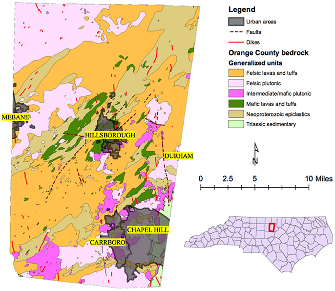
Figure 1. Map of Orange County, North Carolina showing the geology of the county and municipalities located in the county. Inset is a map of North Carolina with Orange County outlined in red.

The hydrogeologic units of Orange County, NC, are generally the same as the bedrock units and flow is dominated by fractures. The regolith layer, that sits atop the bedrock, varies in thickness from 0 to 150 feet and acts as the main reservoir for groundwater in the area due to high porosity and permeability and slowly feeds water down to the fractures in the bedrock aquifers. While some domestic supply wells only tap the regolith aquifer, the majority of wells extend to the bedrock aquifers for higher yields, due to a larger available drawdown area, and the average well depth is around 200 feet. The dominantly crystalline bedrock aquifers are most likely interconnected to some degree due to fracturing and faulting (Cunningham and Daniel, 2001).

Data and Methods

While the EPA does not monitor private wells, the NCDHHS (North Carolina Department of Health and Human Services) and local health departments began sampling private wells in 1999 (Pippin, 2005) under the statewide private well testing program¹. Most of the data used in this study included a database of well water arsenic concentrations in Orange County, a database of water quality characteristics for wells across North Carolina provided by the North Carolina Geological Survey (NCGS), and a detailed bedrock map of Orange County (Bradley et al., 2016). The Orange County data contained 1,335 arsenic concentration analyses of private wells that were geolocated to tax parcel centroids as described in Kim et al. (2011). The statewide well database contained 19,443 samples, but selecting samples only from Orange County reduced the sample size to 769 and these samples were then joined to the more accurately geocoded Orange County well data based on NC DHHS sample number. In these datasets, arsenic concentrations were in units of mg/L and sample concentrations that were below the detection limit of 0.001 mg/L were marked “<0.001”, so a new field was generated to express these values as 0 (zero), since their actual concentration could not be assessed. A new field was created converting the concentration to μg/L (ppb) for ease of examination. Other elemental concentrations and water quality parameters varied in units and detection level and any samples that had variables that were below their respective detection limits were replaced with 0 (zero). The well sample points were then spatially joined to the simplified geologic map. Ultimately, two datasets of private well water in Orange County were obtained. The first dataset contained 1,335 samples of only location and arsenic concentrations and the second dataset contained 769 samples with location, arsenic concentrations, and many more water quality variables.

In order to assess the geologic correlation between arsenic concentrations in groundwater and the bedrock, the geologic units in Orange County were simplified based on general rock type. These six general rock units were: (i) felsic lavas and tuffs, (ii) felsic plutonic, (iii) intermediate/mafic plutonic, (iv) mafic lavas and tuffs, (v) Neoproterozoic epiclastics, and (vi) Triassic sedimentary.

Interpolation Modeling and Pluton Proximity Analysis

Kriging is an advanced geostatistical procedure that can be used to create surfaces of estimated values and probabilities based on a set of scattered points and their values (Davis, 2002). Previous studies such as Pippin (2005) and Yang et al. (2009) have used indicator kriging methods to create probability maps of arsenic concentration ranges in groundwater and studies such as Kim et al. (2011) and Sanders et al. (2012) have used simple and Bayesian kriging methods to create probability and prediction maps. For this study, simple kriging modeling was used to create a prediction map of arsenic concentrations for Orange County using arsenic concentration data from 1,335 private wells to initially observe if an obvious spatial connection existed between certain rock groups and higher or lower concentration predictions. This method was used because it allowed for the transformation of the data to a normal distribution using normal score transformation. Normal score transformation works by ranking the dataset from lowest to highest values and matching these ranks to equivalent ranks from a normal distribution². A normal distribution of the data significantly helps the accuracy of the kriging method because outliers can incorrectly influence kriging interpolations. The various parameters of the prediction model were then subjectively adjusted until the semivariogram model appeared to best fit the averaged semivariogram values. See Figures S1A–C for images of the normal score transformation of the data and the semivariogram modeling and specifications. Geologic units that appeared to be in zones of high prediction values were added to the prediction map to show their possible spatial correlation. Statistics were calculated for arsenic concentration in each geologic unit using the “Summarize” tool.

In addition to the Kriging interpolation modeling, statistical analysis was performed to evaluate well distance to pluton boundaries as another factor in detecting arsenic. Pluton emplacement in Orange County occurred in a four main time periods: (1) Neoproterozoic (ca. 630 Ma); (2) Neoproterozoic (ca. 613–614 Ma); (3) Neoproterozoic (ca. 579 Ma); and (4) during the Cambrian/late Neoproterzoic (ca. 546 Ma). These emplacements occurred after the initial deposition of the felsic lavas and tuffs that occurred around ca. 629–633 Ma. It is possible and likely that these emplacements caused hydrothermal or diagenetic alterations to the surrounding and overlaying rocks and possibly created increased arsenic content at these boundaries. Moreover, Kim et al. (2011) found higher arsenic concentrations likely to occur in wells close to transition zones and faults in Orange County, NC. By using the near tool in ArcGIS, sample locations located within 500 m or less to the plutons were selected and put in a separate shapefile. The rest of the sample locations were also put into a separate shapefile for ease of analysis. A two-tailed Mann-Whitney-Wilcoxon nonparametric test was used to test differences between the arsenic concentrations in wells closer than 500 m to a pluton contact and arsenic concentrations in wells farther than 500 m away from a pluton contact.

Wholerock Sample Collection

Bedrock samples of each simplified geologic unit were collected in order to examine if a direct connection between the concentration of arsenic in bedrock and in groundwater existed. Twenty-six samples were collected in all from the six general units. Five of the 26 samples came from previous NCGS collection. Table S1 provides a summary of the number of samples and sample IDs from each unit.

Whole rock analyses on 49 samples conducted by the NCGS are used to supplement the collected samples (unpublished data from Philip Bradley of the NCGS). The detection limit for arsenic in these analyses was 3 ppm, which is high in comparison to the detection limit of the ICP-MS used in this study, meaning this data may not be as accurate and it is used cautiously to compare arsenic concentrations that were found in this study. Table S2 provides a summary of the number of samples located in each unit and the sample IDs.

Wholerock Sample Preparation/Analysis

Sample preparation for the whole rock analyses involved the use of a rock saw to carefully remove weathered parts of the samples so that a clean and unweathered piece was left. A Chipmunk Jaw Crusher was used to pulverize the unweathered pieces into smaller pieces, which were then powdered using a ball mill. The equipment used in the sample processing stage was meticulously cleaned using water and brushes so cross contamination between samples was minimal or non-existent. Given the high porosity of the Triassic sedimentary rocks, organic arsenic in organic material had the potential to significantly contribute to the overall arsenic content in samples from this unit. Two sets of samples for this unit were created for analyses: one with organic arsenic in the sample and one without organic arsenic in the sample. To incinerate possible organic material that could have been deposited through permeation and weathering, only one set of the Triassic sedimentary samples were put into an oven at 400°C for 3 h in aluminum foil trays. Based on the findings of Gray et al. (2001), the samples were heated to 400°C; this temperature is less than 522°C, the temperature at which inorganic arsenic volatilization was observed, but sufficiently high enough to burn off organic material. In case some inorganic arsenic volatilized during the heating process, both unheated and heated Triassic sedimentary samples were analyzed.

Approximately 50 milligrams of powder was weighed out per sample based on concentration calculations that assumed at least 0.1 ppm of arsenic in each of the samples. Dissolution of the rock powder was done using a step acid digestion method of concentrated hydrofluoric and concentrated nitric acid to initially dissolve the rock powder and then concentrated hydrochloric acid to dissolve the remaining fluoride crystals. In some samples, such as the USGS SBC-1 shale standard, aqua regia (1 part concentrated nitric acid: 3 parts concentrated hydrochloric acid) was used to dissolve the sample if the hydrofluoric and nitric acid mix did not dissolve it completely. During all stages of the acid digestion, the samples were sealed in beakers and placed on a hot plate at ~140°C and were dried down in between steps at approximately 80°C. After residual material and fluoride crystals were dissolved and the samples were dried down, the samples were prepped for analysis on an ICP-MS by diluting them in 5 ml of 2 v/v% nitric acid and then again by taking 1 ml of this solution and diluting it in another 4 ml of 2 v/v % nitric acid. This was done to reduce the matrix percentage and avoid interferences on the ICP-MS. Helium gas was also used in addition to the carrying argon gas to reduce plasma- and matrix-based polyatomic interferences in both iron and arsenic analysis as utilized by Dial et al. (2015). Standard calibration solutions were made for both arsenic and iron after an initial calibration run. Table S3 shows the calculated concentrations of each of the diluted standards after using a scale to initially weigh out the volume of standard used for dilution. Arsenic and iron concentration analysis of the samples and standards was done using an Agilent 7900 Q-ICP-MS at the Plasma Mass Spectrometry Laboratory at the University of North Carolina at Chapel Hill. Percentage accuracy of arsenic concentration was calculated using a USGS shale standard, SBC-1. The accuracy was determined to be 8.4% when compared to its certified value. Table S4 provides the calculated concentrations and percentage errors of the As and Fe analysis for the SBC-1 reference standard.

Multivariate Analysis

To further analyze the occurrence of arsenic in groundwater in Orange County, multivariate analysis was performed on a dataset of 21 variables from 769 wells in Orange County. These variables included 12 water chemical parameters, distances from each well sample point to the nearest rock unit for each of the six units, and the average arsenic concentrations from each rock type from this study's sample analysis, the NCGS sample analysis, and the mean of the two analyses. Due to the number of wells with undetectable arsenic, arsenic was not well correlated with any of the variables. Hierarchical cluster analysis (HCA) and principal component analysis (PCA) was used instead to reveal possible patterns in the dataset. Hierarchical cluster analysis and principal component analysis have previously been used to identify geochemical controls on groundwater and specifically in arsenic contamination studies such as Kouras et al. (2007), Sappa et al. (2014), and Jiang et al. (2015) by reducing datasets and identifying variables associated with groundwater arsenic. In this study, PCA was used to determine if relationships existed between arsenic and any of the other variables. By studying this relationship, a geochemical release mechanism could be found that explains the presence of arsenic in groundwater in Orange County, North Carolina.

Hierarchical clustering is a method of analysis that joins the most similar observations, then successively connects the next most similar observations to these. The analysis uses square (n × n) matrices to repeatedly calculate similarities between observations, and observations with the highest similarities are merged at each calculation step. The progression of these computations are displayed as a dendrogram that exhibit distinct clusters of similar observations (Davis, 2002). This analysis was used to initially reduce the number of variables for the dataset that would be used for the subsequent principal component analysis (PCA) and eliminated variables such as well distance from bedrock units and some chemical variables of the groundwater.

Principal component analysis (PCA) is an eigenvector-based multivariate analysis that works by orthogonally transforming datasets of potentially correlated variables into uncorrelated variables called principal components. Eigenvalues of these principal components reveal how much percentage of the variance in the original dataset each principal component explains. The first principal component explains the highest percentage of variance and the following components explain decreasing percentages (Davis, 2002). The eigenvectors, also known as loadings, of each principal component then reveal the relative contribution from each of the original variables to the principal component. Plots of the first two principal components, the components that explain the most variance, can then show groups of variables that are similar or positively correlated with one another (Sappa et al., 2014). This type of analysis can be very useful for determining rough associations between variables and predicting mobilization mechanisms of trace elements, such as arsenic.

When associations and groupings were determined using principal component analysis (PCA), statistical tests were performed to test differences between groups. Shapiro-Wilk tests were performed first to determine normality of the variables. If the variables were not normally distributed, nonparametric Mann-Whitney-Wilcoxon tests were performed to test if there were significant statistical differences between variables. All statistical tests were performed at the 95% confidence interval. Ultimately, the variables pH, F⁻, alkalinity, Mg²⁺, Ca²⁺, and hardness were selected to test mean differences between wells with no detected arsenic and wells with detected arsenic.

Results

Modeling and ICP-MS Analysis

Initial mapping of arsenic concentrations for each private well point from the 1,335 samples in Orange County (Figure 2) appears to show that clustering or directionality exists in wells with similar concentrations of arsenic. Generally, it appears that most of the wells in plutonic bodies have arsenic concentrations below detection limit (<1 μg/L) and that most of the wells with detectable arsenic reside in the felsic lavas and tuffs or Neoproterozoic epiclastics units. Table S5 provides a summary of the number of wells in each unit and the average arsenic concentrations per well in each unit. Through arsenic concentration prediction mapping using simple kriging, this relationship becomes more obvious. Figure 3 shows what appears to be a good spatial overlap of the higher arsenic concentration prediction contours and the Neoproterozoic epiclastics and that the general direction of arsenic contamination trends northeast with the Carolina Terrane. However, there are pockets of higher arsenic predictions in the Neoproterozoic epiclastics and a minor northwest direction to arsenic predictions.

FIGURE 2

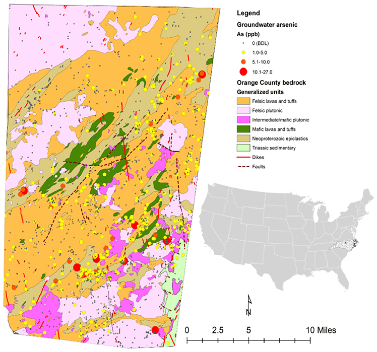
Figure 2. Generalized geologic map of Orange County with the well data of arsenic concentrations from groundwater sample data obtained through the NC DHHS. The red dot on the US map indicates the location of the Orange County.

FIGURE 3

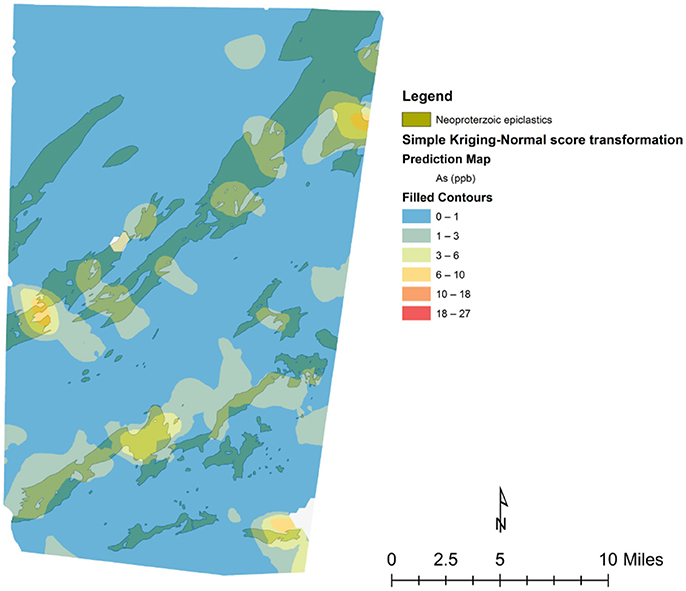
Figure 3. Neoproterozoic epiclastics unit underlying the arsenic concentration prediction map created with the simple kriging method.

This observed spatial connection between the Neoproterozoic epiclastics and high-predicted arsenic, as well as high average arsenic concentrations in groundwater in the mafic lavas and tuffs and Neoproterozoic epiclastics, could possibly mean that a relationship between the average arsenic concentration in rock and the average arsenic content in groundwater exists. By analyzing arsenic concentrations of whole rock samples from each rock type, mean arsenic concentrations for each rock type were calculated (Table 1). Previous whole rock analyses by the North Carolina Geological Survey (NCGS) of 49 samples were also examined (Table 2), but kept separate from the current dataset to see if there was a difference. Overall, higher variations exist in mean arsenic concentrations across rock types from the previous NCGS analyses compared to the analyses from this study (Figure 4).

TABLE 1

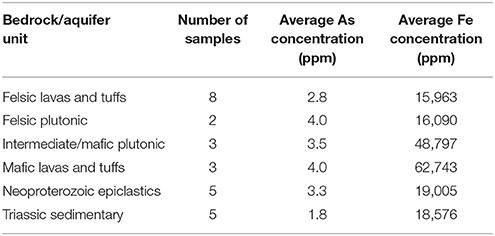
Table 1. The average arsenic and iron concentrations in the bedrock unit samples from this study.

TABLE 2

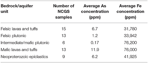
Table 2. The average arsenic and iron concentrations in the bedrock unit samples from the NCGS analyses.

FIGURE 4

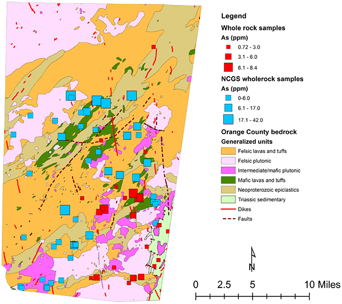
Figure 4. Generalized map of Orange County showing sampling locations from this study (red boxes) and previous NCGS whole rock analysis (blue boxes).

Iron and arsenic concentrations in samples analyzed in this study correlate positively in each generalized rock unit, meaning that arsenic is likely associated with iron in the mineralogy. This relationship is not as clear in the whole rock samples previously analyzed through the NCGS. Figures S2A,B show the raw data with no correlation lines for both sets of analyses.

Examining relationships between average groundwater arsenic concentration in each rock unit and the average arsenic whole rock content for each rock yields a strong relationship within the NCGS samples (R² = 0.7) and no relationship within samples analyzed from this study (R² = 0.2). Figures S3A,B show the plots for this data and the linear relationships between the variables.

Pluton Proximity Analysis

The two-tailed Mann-Whitney Wilcoxon test used to test differences between the arsenic concentrations in wells closer than 500 m to pluton boundaries and wells greater than 500 m away from pluton boundaries found a difference in the mean arsenic concentrations of the two groups. The results show that wells located greater than 500 m from pluton boundaries had a statistically greater mean at the 95% confidence interval. Figure S4 and Table S6 detail the wells selected and the statistical parameters used for the analysis.

Multivariate Analysis

From the ICP-MS analyses, it seemed that arsenic concentrations in the bedrock do not directly relate to arsenic concentrations in the groundwater meaning that some other factor must be influencing arsenic concentrations in the groundwater. By using hierarchical clustering analysis, 21 variables that could be affecting or associated with arsenic in groundwater from the wells were analyzed by creating a dendrogram with groupings of associated variables. This cluster analysis helped to reduce the 21 variables to only 6 variables that were more closely associated with arsenic. These variables were Mg²⁺ (mg/L), Ca²⁺ (mg/L), hardness, F⁻ (mg/L), alkalinity, and pH. Figure S5 shows the dendrogram created through the hierarchical clustering analysis.

Based on this new group, Q-mode principal component analysis was performed to look at patterns of similarity in the samples by the variables in the new group. This analysis showed that the first two principal components (1 and 2) explain approximately 64.8% of the variance in the dataset as shown in Figure S6. Bi-plots of the Q-mode analysis were created to plot variables and samples and to assess other groupings within the samples, such as rock grouping and arsenic detection in the sample. The sample points in the bi-plot are plotted by their scores in principal components 1 and 2 and the variable vectors are plotted by their loadings in principal component 1 and 2. Sample points that are close together correspond to observations that have similar scores on the components displayed in the plot and if the points fit the variables well then they will plot closer to it. Likewise, variable vectors that point in the same general direction have positive correlation and negative correlation if they point opposite to each other. In Figure 5, the variables Mg²⁺, Ca²⁺, and hardness all point in the same general direction and the variables As, pH, F⁻, and alkalinity all point in the same general direction with approximately the same length, indicating that these groups are more correlated to one another. Also in Figure 5, the sample points are distinguished by the bedrock unit in which they are located and ellipses containing 68% of samples of each bedrock type do not seem to create distinguishable groups based on the principal components; thus not much variability in these groups is explained by these variables. In Figure 6, a moderately distinct grouping is observed between wells with detected and non-detected arsenic. Although there is some overlap in the groups, the differences in these groups were examined for all 6 variables, especially pH, As, F⁻, and alkalinity, because the greatest shift in the groups is seen in the direction of those variables. Shapiro-Wilk tests concluded that most of the variables for each group were not normally distributed and Mann-Whitney-Wilcoxon tests for the paired variables from the two groups all showed that there was significant difference between the groups at the 95% confidence interval. Table S7 provides a summary of the means of each variable for each group and if there was significant difference.

FIGURE 5

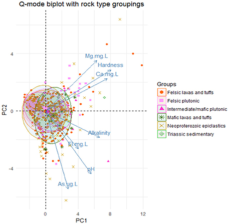
Figure 5. Q-mode PCA analysis biplot of the 1st two principal components. Ellipses were drawn around the points from each rock group encompassing 68% of the points in each group with each ellipse.

FIGURE 6

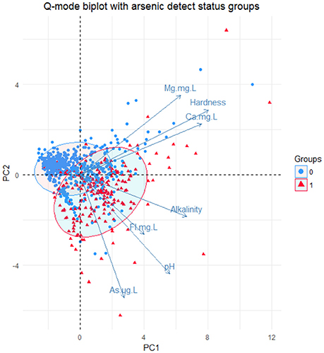
Figure 6. Q-mode PCA analysis biplot of the 1st two principal components. Ellipses were drawn around the points from each detect group encompassing 68% of the points in each group with each ellipse. Group = 0 = no detect, Group = 1 = detect.

Discussion

Simple kriging modeling indicates that a spatial connection exists between the Neoproterozoic epiclastics and areas of higher predicted arsenic. This connection suggests that this unit is likely the most responsible for natural arsenic contamination of groundwater in Orange County, NC. Figure 3 shows the simple kriging prediction model and generally, the areas with higher predicted arsenic concentrations in groundwater are within the Neoproterozoic epiclastics unit. Furthermore, the higher predicted zones trend mostly in a northeast-southwest direction, similar to the trend of the Carolina Terrane. This directionality was also noted by Kim et al. (2011). Also in support of this connection is the high average arsenic concentration for wells in the Neoproterozoic epiclastics found in Table S5. While the mafic lavas and tuffs and Triassic Sedimentary units have higher averages, they may not be as reliable given their small sample size. With over 300 well samples located in the Neoproterozoic epiclastics unit, the average of 1.25 μg/L is more reliable and much higher than most of the other units. In regards to potential error, there is a minor northwest directionality to the predicted values and the higher predicted arsenic zones are patchy and do not completely match the Neoproterozoic epiclastics unit. This could be explained by error produced from the simple kriging modeling through incorrect extrapolation of sample values if a single point has a high value or if there is an uneven distribution of points. In this prediction model, errors may come from uneven sampling and a highly non-normal sampling distribution. Other possibilities for error are that the hydrogeologic units do not directly match the bedrock that is mapped and other variables besides bedrock types are involved with arsenic concentrations in well water and are affecting its release in specific locations within the Neoproterozoic epiclastics unit. For example, fractures and preferential pathways of flow may spread arsenic from one type of bedrock to another, thus obscuring the origin of the arsenic. In addition to the kriging prediction model, the pluton proximity analysis revealed that wells located within 500 m to pluton contact zones do not have higher arsenic concentrations and average concentrations of arsenic are statistically higher 500 m or farther from pluton contacts. Our results suggest that arsenic concentrations in groundwater near pluton contact zones are not higher, in contrast with the findings of Kim et al. (2011) that showed wells close to transition zones and faults had a higher probability of containing detectible arsenic. Kim et al. (2011) also found that the welded tuff and hydrothermal quartz bodies were associated with higher concentrations of arsenic, which was not observed in this study. These discrepancies between results can possibly be explained by different sorting criteria for bedrock types, different well datasets, different modeling techniques, and different geologic maps. For instance, Kim et al. (2011) only had access to an incomplete and older geologic map of Orange County, only used 471 well points for their prediction model, and used different spatial modeling techniques. The differences in the data and techniques used between studies could easily influence differences in the prediction outcome. Future modeling efforts should be made using an updated dataset of well points to create a more accurate prediction model and reassess proximity concentrations near contacts and fault zones. Well depth would also be an important variable to consider in future modeling, as Kim et al. (2011) found increased concentrations of arsenic in deeper wells in Orange County, NC.

Neither the whole rock analyses from the NCGS nor this study revealed any results that would lead to the conclusion that a specific rock unit was responsible for the elevated arsenic concentrations in well water. This result agrees with Smedley and Kinniburgh (2002) who suggested there is not a direct relationship between arsenic concentrations in groundwater and in the bedrock aquifer, indicating high arsenic in bedrock does not mean high arsenic in groundwater within that bedrock unit and vice versa. Our whole rock analysis results contradict with the previous results from the NCGS. The NCGS sample data indicates a strong positive correlation between arsenic concentrations in rocks and groundwater (Figure S6A), while the sample data from this study shows no, or weak, correlation (Figure S6B). A number of factors could be influencing these discrepancies including inaccurate analysis of whole rock samples, lack of whole rock and water samples for some units leading to incorrect average assumptions, and the absence of Triassic sedimentary whole rock samples in the NCGS analysis. It may also be incorrect to directly compare groundwater arsenic concentrations and bedrock arsenic concentrations if hydrogeological and bedrock units in Orange County differ from one another and if other variables are responsible for preferential release of arsenic in certain rock types.

Our whole rock analysis reveals a correlation between iron and arsenic concentrations in these samples. In both analyses, arsenic concentrations increase as iron content increases, as seen in Figures S2A,B. This relationship was noted in Abraham (2009), suggesting that arsenic is associated with iron-bearing minerals such as arsenopyrite and iron oxyhydroxides. In support of this assumption, small pyrite crystals were observed in some of the samples from the felsic lavas and tuffs unit, although no analyses were done to confirm the existence of arsenic-bearing iron oxyhydroxides or arsenic-bearing pyrite in any unit. However, Abraham (2009) confirmed the existence of pyrite and Fe and Mn oxides along veins and fractures in cores of the bedrock from Union County, NC and observed increasing sulfide mineralogy as depth increased. Another key factor to consider when examining this relationship is the differing iron concentrations in each unit. For example, the intermediate/mafic plutonic and mafic lavas and tuffs units have much higher iron content than the other units due to mineralogy not associated with arsenic, but offsetting them from the rest of the units. More thorough analyses, including more samples and more elemental analysis, should be done in the future to correctly classify the dominant arsenic-bearing minerals in each unit. In addition, analysis of weathered and unweathered surfaces should be conducted to see if the dominant arsenic-bearing mineralogy changes.

Multivariate analyses of 769 wells and 21 variables (Figures 5, 6) indicate that arsenic is associated mostly with pH, alkalinity, and fluorine, and partially with hardness, magnesium, and calcium. All of these variables are statistically different between detect and non-detect arsenic wells when tested using a non-parametric test at the 95% confidence interval, and all show higher means in the arsenic-detected wells. These associations make sense from a geochemical perspective because the dominant factors influencing arsenic speciation and mobilization in water are pH, redox potential, alkalinity, and total dissolved solids. Increased pH and alkalinity in groundwater can lead to desorption of arsenic from metal oxyhydroxides (Hinkle and Polette, 1999; Welch et al., 2000) and are also correlated with arsenic in oxidizing environments (Bundschuh et al., 2004; Gomez et al., 2009). Release of arsenic through anion exchange processes between arsenic-bearing minerals and inorganic anions, such as F⁻ and bicarbonate, has been observed in volcanic rocks (Abraham, 2009; Casentini et al., 2010) also observed increased arsenic in groundwater with increased pH in Union County, NC.

Given the geochemical evidence, we suggest that arsenic being released from bedrock aquifers in Orange County, NC is primarily due to oxidation of arsenic-bearing sulfide minerals in the Neoproterozoic epiclastics unit and partially from the felsic lavas and tuffs unit. Characteristics of the groundwater in arsenic-contaminated oxidizing regions include neutral to high pH, high salinity, oxidizing conditions, low Fe and Mn, and correlation between anions and oxyanions such as F⁻ and ${\text{HCO}}_3^{-}$ and arsenic (Nicolli et al., 2012; Smedley and Kinniburgh, 2013). Most of these characteristics match the geochemical associations of groundwater arsenic observed in Orange County, NC. Furthermore, high arsenic has been shown to be associated with felsic volcanic rocks and volcanogenic sediments in oxidizing environments (Bundschuh et al., 2004; Gomez et al., 2009; Nicolli et al., 2012) and the geology of Orange County is dominated by felsic volcanic rocks and metamorphosed volcanogenic sediments, including the felsic lavas and tuffs and Neoproterozoic epiclastics units. It is therefore proposed that millions of years ago initial oxidation of arsenic-bearing sulfides occurred in felsic volcanic rocks, such as the felsic lavas and tuffs unit, due to weathering. The weathered volcanic material was then deposited and formed the Neoproterozoic epiclastics, simultaneously depositing arsenic in authigenic arsenic-bearing sulfides and secondary minerals, such as metal oxyhydroxides. It is also possible that post-depositional fluids emplaced sulfide minerals in the unit during the subsequent periods of volcanism and metamorphism. Today, this arsenic is most likely being released into groundwater primarily through oxidation of authigenic sulfide minerals in the Neoproterozoic epiclastics unit, although oxidation of primary sulfide minerals in the felsic lavas and tuffs unit may also contribute arsenic. Oxidation of sulfide minerals and mobilization of arsenic in these units may be aided by existing fractures and well boreholes as suggested by Schreiber et al. (2000); Abraham (2009), and Bondu et al. (2017). While the majority of bedrock in Orange County, NC is crystalline with low permeability and secondary porosity, the Neoproterozoic epiclastics unit likely has much higher permeability and porosity due to its depositional history and only low-grade metamorphism. This is consistent with the observation that the collected samples of the Neoproterozoic epiclastics unit were much more fractured than samples of the other crystalline units. In regards to oxidation from well boreholes, Abraham (2009) observed increasing sulfide mineral concentrations in deeper cores in Union County, NC, meaning deeper wells have the potential to oxidize a greater amount of arsenic-bearing sulfide minerals, leading to higher arsenic concentrations in groundwater from deeper wells. This may be the reason why Kim et al. (2011) observed and predicted higher arsenic concentrations from deeper wells. To clarify, groundwater in Orange County, NC does contain small concentrations of arsenic but does not exhibit the high arsenic concentrations that are observed in oxidizing environments with semi-arid climates, young volcanic or loess aquifers, and long residence times (Nicolli et al., 2012; Smedley and Kinniburgh, 2013). Instead, the subtropical climate of Orange County, NC most likely helps dilute arsenic concentrations and it is possible that most of the arsenic in the bedrock units has been oxidized already given the age of the bedrock. Desorption from arsenic adsorbed onto metal oxyhydroxides due to high alkalinity, increased F⁻, and increased pH may also contribute arsenic to groundwater (Nicolli et al., 2012; Smedley and Kinniburgh, 2013; Khair et al., 2014; Bondu et al., 2017). Desorption may not be the main mechanism of release because the characteristic features of arsenic contamination from reductive dissolution, such as high Fe and Mn and young, alluvial host aquifers (Smedley and Kinniburgh, 2013), are not observed in Orange County, NC.

Although the correlations between arsenic and these variables are weak and the multivariate analyses explain only 65% of the variance in the dataset, the analyses support arsenic is mainly introduced into groundwater by a geochemical release driven by oxidation of arsenic from arsenic-bearing sulfide minerals in the Neoproterozoic epiclastics unit and in some areas of the felsic lavas and tuffs unit in Orange County, NC. In order to clarify these assertions, future water quality analyses should be done on groundwater throughout Orange County comprising more analyses such as dissolved oxygen concentrations, redox potential, arsenic speciation, and better detection limits for arsenic and other trace elements, along with mineral identification.

Conclusion

This study found some potential mechanisms for natural arsenic release into groundwater in Orange County, NC involving an association of observed arsenic in wells and higher pH, alkalinity, F⁻, and hardness. Furthermore, simple kriging modeling has revealed a spatial relationship between the Neoproterozoic epiclastics unit and higher predicted arsenic. It is clear from the PCA analysis that higher pH, alkalinity, and F⁻ are mostly associated with arsenic in groundwater, whereas variables such as distance from each rock type and average whole rock arsenic concentration in each unit are not correlated to arsenic concentration in groundwater. The geochemical characteristics of groundwater in Orange County closely mimic the geochemical characteristics observed in semi-arid inland basins, but in a diminished way because of the climactic, hydrologic, and bedrock age differences. From this spatial and chemical relationship, this study proposes a connection between the Neoproterozoic epiclastics unit in Orange County, NC and higher arsenic concentrations in groundwater within and in close proximity to the unit. These elevated arsenic concentrations found within the unit are thought to be primarily due to oxidation of authigenic arsenic-bearing sulfide minerals in the unit and partly from desorption of arsenic from metal oxyhydroxides.

Author Contributions

ED and X-ML designed the study. ED collected the samples, analyzed samples, and data sets. ED wrote the manuscript with considerable input from X-ML.

Conflict of Interest Statement

The authors declare that the research was conducted in the absence of any commercial or financial relationships that could be construed as a potential conflict of interest.

The reviewer RF and handling editor declared their shared affiliation at the time of review.

Acknowledgments

This research was supported by a startup grant and a Junior Faculty Development Award awarded to X-ML by the University of North Carolina at Chapel Hill. Phil Bradley helped with the fieldwork. Ryan Mills is thanked for the help in the clean lab and Cheng Cao for her help with ICP-MS analysis. Heather Hanna and Clement Bataille provided useful discussion. We thank the editor and two reviewers for providing helpful comments to improve the paper.

Supplementary Material

The Supplementary Material for this article can be found online at: https://www.frontiersin.org/articles/10.3389/feart.2018.00111/full#supplementary-material

Footnotes

1. ^NCDEQ. Private Well Water Quality. Available online at: https://deq.nc.gov/about/divisions/water-resources/water-quality-regional-operations/groundwater-protection/ground-water-quality-monitoring/private-well-water-quality (Accessed December 2016).

2. ^ArcGIS Desktop Help 9.3. Normal Score Transformation. Available online at: http://webhelp.esri.com/arcgisdesktop/9.3/index.cfm?TopicName=Normal%20score%20transformation (Accessed April 2017).

References

Abraham, J. (2009). A Hydrogeological Assessment of Arsenic in the Carolina Terrane of Union County, North Carolina. North Carolina Division of Water Quality, Groundwater Circular 2009-01. 1–40.

Biswas, A., Hendry, M. J., and Essilfie-Dughan, J. (2016). Geochemistry of arsenic in low sulfide-high carbonate coal waste rock, Elk Valley, British Columbia, Canada. Sci. Total Environ. 579, 396–408. doi: 10.1016/j.scitotenv.2016.11.084

PubMed Abstract | CrossRef Full Text | Google Scholar

Bondu, R., Cloutier, V., Rosa, E., and Benzaazoua, M. (2017). Mobility and speciation of geogenic arsenic in bedrock groundwater from the Canadian Shield in western Quebec, Canada. Sci. Total Environ. 574, 509–519. doi: 10.1016/j.scitotenv.2016.08.210

PubMed Abstract | CrossRef Full Text | Google Scholar

Bradley, P. J., Hanna, H. D., Gay, N. K., Stoddard, E. F., Bechtel, R., Phillips, C. M., et al. (2016). Geologic Map of Orange County, North Carolina. North Carolina Geological Survey Open-file Report 2016-05, scale 1:50,000, in color.

Brown, K. G., and Ross, G. L. (2002). Arsenic, drinking water, and health: a position paper of the american council on science and health. Regul. Toxicol. Pharmacol. 36, 162–174. doi: 10.1006/rtph.2002.1573

PubMed Abstract | CrossRef Full Text | Google Scholar

Bundschuh, J., Farias, B., Martin, R., Storniolo, A., Bhattacharya, P., Cortes, J., et al. (2004). Groundwater arsenic in the Chaco-Pampean Plain, Argentina: Case study from Robles County, Santiago del Estero Province. Appl. Geochem. 19, 231–243. doi: 10.1016/j.apgeochem.2003.09.009

CrossRef Full Text | Google Scholar

Casentini, B., Pettine, M., and Millero, F. J. (2010). Release of arsenic from volcanic rocks through interactions with inorganic anions and organic ligands. Aquat. Geochem. 16, 373–393. doi: 10.1007/s10498-010-9090-3

CrossRef Full Text | Google Scholar

Cunningham, W. L., and Daniel, C. C. III. (2001). Investigation of Ground-Water Availability and Quality in Orange County, North Carolina. Available online at: https://nc.water.usgs.gov/reports/wri004286/pdf/report.pdf (Accessed December 2016).

Davis, J. C. (2002). Statistics and Data Analysis in Geology. New York, NY: John Wiley & Sons.

Dial, A. R., Misra, S., and Landing, W. M. (2015). Determination of low concentrations of iron, arsenic, selenium, cadmium, and other trace elements in natural samples using an octopole collision/reaction cell equipped quadrupole-inductively coupled plasma mass spectrometer. Rapid Commun. Mass Spectrom. 29, 707–718. doi: 10.1002/rcm.7152

PubMed Abstract | CrossRef Full Text | Google Scholar

Gomez, M. L., Blarasin, M. T., and Martínez, D. E. (2009). Arsenic and fluoride in a loess aquifer in the Central Area of Argentina. Environ. Geol. 57, 143–155. doi: 10.1007/s00254-008-1290-4

CrossRef Full Text | Google Scholar

Gray, D. B., Watts, F., and Overcamp, T. J. (2001). Volatility of arsenic in contaminated clay at high temperatures. Environ. Eng. Sci. 18, 1–7. doi: 10.1089/109287500750070216

CrossRef Full Text | Google Scholar

Hinkle, S. R., and Polette, D. J. (1999). Arsenic in Ground Water of the Willamette Basin, Oregon. USGS, Water-Resources Investigation Report 98–4205.

Jiang, Y., Guo, H., Jia, Y., Cao, Y., and Hu, C. (2015). Principal component analysis and hierarchical cluster analyses of arsenic groundwater geochemistry in the Hetao basin, Inner Mongolia. Chemie der Erde Geochem. 75, 197–205. doi: 10.1016/j.chemer.2014.12.002

CrossRef Full Text | Google Scholar

Khair, A. M., Li, C., Hu, Q., Gao, X., and Wanga, Y. (2014). Fluoride and arsenic hydrogeochemistry of groundwater at Yuncheng basin, Northern China. Geochem. Int. 52, 868–881. doi: 10.1134/S0016702914100024

CrossRef Full Text | Google Scholar

Kim, D., Miranda, M. L., Tootoo, J., Bradley, P., and Gelfand, A. E. (2011). Spatial modeling for groundwater arsenic levels in North Carolina. Environ Sci. Technol. 45, 4824–4831. doi: 10.1021/es103336s

PubMed Abstract | CrossRef Full Text | Google Scholar

Kouras, A., Katsoyiannis, I., and Voutsa, D. (2007). Distribution of arsenic in groundwater in the area of Chalkidiki, Northern Greece. J. Hazard. Mater. 147, 890–899. doi: 10.1016/j.jhazmat.2007.01.124

PubMed Abstract | CrossRef Full Text | Google Scholar

Maascheleyn, P. H., Delaune, R. D., and Patrick, W. H. (1991). Effect of redox potential and pH on arsenic speciation and solubility in a contaminated soil. Environ. Sci. Technol. 25, 1414–1419.

Google Scholar

McCarty, K. M., Hanh, H. T., and Kim, K. (2011). Arsenic geochemistry and human health in South East Asia. Rev. Environ. Health 26, 71–78. doi: 10.1515/reveh.2011.010

PubMed Abstract | CrossRef Full Text | Google Scholar

Murray, J., Nordstrom, D. K., Dold, B., and Kirschbaum, A. (2016). “Distinguishing potential sources for As in groundwater in Pozuelos Basin, Puna region Argentina,” in Arsenic Research and Global Sustainability, eds P. Bhattacharya, M. Vahter, J. Jarsjö, J. Kumpiene, A. Ahmad, C. Sparrenbom, G. Jacks, M. E. Donselaar, J. Bundschuh, and R. Naidu (London: Taylor and Francis Group), 94–96.

Google Scholar

Naujokas, M. F., Anderson, B., Ahsan, H., Aposhian, H. V., Graziano, J. H., Thompson, C., et al. (2013). The broad scope of health effects from chronic arsenic exposure: update on a worldwide public health problem. Environ. Health Persepect. 121, 295–302. doi: 10.1289/ehp.1205875

PubMed Abstract | CrossRef Full Text | Google Scholar

Nicolli, H. B., Bundschuh, J., Blanco, M. D. C., Tujchneider, O. C., Panarello, H. O., Dapeña, C., et al. (2012). Arsenic and associated trace-elements in groundwater from the Chaco-Pampean plain, Argentina: results from 100 years of research. Sci. Total Environ. 429, 36–56. doi: 10.1016/j.scitotenv.2012.04.048

PubMed Abstract | CrossRef Full Text | Google Scholar

Nordstrom, D. K. (2002). Worldwide occurrences of arsenic in ground water. Science 296, 2143–2145. doi: 10.1126/science.1072375

PubMed Abstract | CrossRef Full Text | Google Scholar

Pippin, C. G. (2005). “Distribution of total arsenic in groundwater in the North Carolina Piedmont,” in NWGA Naturally Occurring Contaminants Conference. Arsenic, Radium, Radon, and Uranium (Charleston, SC), 89–102.

Private Drinking Water Wells (2018). EPA. Available online at: https://www.epa.gov/privatewells (Accessed May 2018).

Sanders, A. P., Messier, K. P., Shehee, M., Rudo, K., Serre, M. L., and Fry, R. C. (2012). Arsenic in North Carolina: public health implications. Environ. Int. 38, 10–16. doi: 10.1016/j.envint.2011.08.005

PubMed Abstract | CrossRef Full Text | Google Scholar

Sappa, G., Ergul, S., and Ferranti, F. (2014). Geochemical modeling and multivariate statistical evaluation of trace elements in arsenic contaminated groundwater systems of Viterbo Area, (Central Italy). Springerplus 3:327. doi: 10.1186/2193-1801-3-237

PubMed Abstract | CrossRef Full Text | Google Scholar

Schreiber, M. E., Simo, J. A., and Freiberg, P. G. (2000). Stratigraphic and geochemical controls on naturally occurring arsenic in groundwater, eastern Wisconsin, USA. Hydrogeol. J. 8, 161–176. doi: 10.1007/s100400050003

CrossRef Full Text | Google Scholar

Smedley, P. L., and Kinniburgh, D. G. (2002). A review of the source, behavior and distribution of arsenic in natural waters. Appl. Geochem. 17, 517–568. doi: 10.1016/S0883-2927(02)00018-5

CrossRef Full Text | Google Scholar

Smedley, P. L., and Kinniburgh, D. G. (2013). “Arsenic in Groundwater and the Environment,” in Essentials of Medical Geology: Revised Edition, ed O. Selinus (Oxfordshire: British Geological Survey), 279–310.

Google Scholar

Tseng, C. H. (2005). Blackfoot disease and arsenic: a never-ending story. J. Environ. Sci. Health C Environ. Carcinog. Ecotoxicol. Rev. 23, 55–74. doi: 10.1081/GNC-200051860

PubMed Abstract | CrossRef Full Text | Google Scholar

USEPA (2001). Technical Fact Sheet: Final Rule for Arsenic in Drinking Water. Available online at: https://nepis.epa.gov/Exe/ZyPdf.cgi?Dockey$=$20001XXE.txt (Accessed December, 2016).

Welch, A. B., Westjohn, D. B., Helsel, D. R., and Wanty, R. B. (2000). Arsenic in groundwater of the United States: occurrence and geochemistry. Groundwater 38, 589–604. doi: 10.1111/j.1745-6584.2000.tb00251.x

CrossRef Full Text | Google Scholar

World Health Organization (2016). Arsenic: Fact Sheet. Available online at: http://www.who.int/mediacentre/factsheets/fs372/en/ (Accessed December 2016).

Yang, Q., Jung, H. B., Culberson, C. W., Marvinney, R. G., Loiselle, M. C., Locke, D. B., et al. (2009). Spatial pattern of groundwater arsenic occurrence and association with bedrock geology in Greater Augusta, Maine. Environ. Sci. Technol. 43, 2714–2719. doi: 10.1021/es803141m

PubMed Abstract | CrossRef Full Text | Google Scholar

Yunus, F. M., Khan, S., Chowdhury, P., Milton, A. H., Hussain, S., and Rahman, M. (2016). A review of groundwater arsenic contamination in Bangladesh: the millennium development goal era and beyond. Int. J. Environ. Res. Public Health 13:215. doi: 10.3390/ijerph13020215

PubMed Abstract | CrossRef Full Text | Google Scholar