Enhanced Core-Mantle Coupling Due to Stratification at the Top of the Core

1. Introduction

Stable stratification at the top of Earth's core suppresses radial motion in the vicinity of the core-mantle boundary (CMB). Weak radial motion may still be present due to magnetic waves that propagate with periods of 100 years or less (Bloxham, 1990; Braginsky, 1993). Detection of these waves in secular variation of the geomagnetic field offers a unique probe of the core near the CMB (Buffett, 2014). Several geomagnetic field models (Jackson et al., 2000; Gillet et al., 2009; Wardinski and Lesur, 2012) support the existence of waves and yield broadly consistent estimates for the strength and thickness of stratification (Buffett et al., 2016), although other interpretations are possible (More and Dumberry, 2018). A nominal value for the layer thickness is 140 km.

Stratification also affects the morphology of the geomagnetic field. Geodynamo models predict an increase in the amplitude of the dipole field relative to the non-dipole components in the presence of stratification (Sreenivasan and Gubbins, 2008; Olson et al., 2017). Stratification can also affect the equatorial symmetry of the geomagnetic field or the relative distribution of zonal and non-zonal field components (Christensen et al., 2010). Comparisons of model predictions with observations of the modern geomagnetic field suggest that stratification cannot exceed 400 km in thickness (Olson et al., 2017; Christensen, 2018).

A more stringent constraint on stratification comes from the time dependence of reversed flux patches at the CMB (i.e., local regions where the radial field is opposite to that expected for a dipole field). Growth of reversed flux patches has been attributed to the expulsion of magnetic field from the core by radial motion (Bloxham, 1986). The rate of growth is controlled by magnetic diffusion, and this process becomes prohibitively slow when radial motion is suppressed within 100 km of the CMB (Gubbins, 2007). While thicker layers are inferred from the detection of waves, these results are not strictly incompatible because both inferences are subject to large uncertainties. Moreover, the presence of waves can contribute to the rate of flux expulsion by allowing weak radial motion on timescales of 101 years to 102 years. The same radial motion may also contribute to other geomagnetic observations that favor limited radial motion near the CMB (Amit, 2014; Lesur et al., 2015).

Core-mantle coupling is also affected by stratification. Transfer of angular momentum across the CMB is commonly invoked to explain changes in LOD over periods of several decades (Gross, 2015). Possible mechanisms include topographic (Hide, 1969; Moffatt, 1977), electromagnetic (Bullard et al., 1950; Rochester, 1962) and gravitational (Jault et al., 1988; Buffett, 1996) torques. Topographic torques are ineffective when the flow around topography is geostrophic because the resulting fluid pressure is equal on the leading and trailing side of bumps (Jault and Finlay, 2015). As a result, the net horizontal force exerted on topography vanishes. Relaxing the condition of geostrophy, particularly by including the influences of a magnetic field, can restore the topographic torque (Anufriyev and Braginski, 1977), although plausible values for the magnetic field suggest that the resulting torques are small (Mound and Buffett, 2005).

Electromagnetic torques are a viable explanation for the LOD variations, as long as the conductance of the lower mantle exceeds 108 S (Holme, 1998). The origin of this conductive material on the mantle side of the boundary is not currently known. Suggestions include unusual mantle mineralogy (Ohta et al., 2010; Wicks et al., 2010), infiltration of core material (Buffett et al., 2000; Kanda and Stevenson, 2006; Otsuka and Karato, 2012) and partial melt (Lay et al., 1998; Miller et al., 2015).

Gravitational coupling between the mantle and fluid core is probably too weak to account for the LOD variations because density variations in the fluid core are expected to be very small (Stevenson, 1987). However, gravitational coupling between the mantle and the inner core can be effective (Buffett, 1996). One restriction on this particular form of gravitational coupling is that fluid motions must first transfer momentum to the inner core by electromagnetic coupling. This momentum is then transferred to the mantle by gravitational coupling to the inner core. Because fluid motion in the core tends to be nearly invariant in the direction of the rotation axis (Jault, 2008), there are large regions of the fluid core that do not directly couple to the inner core. Evidence for changes in length of day associated with torsional waves (Gillet et al., 2010) favor a more general process because waves that do not directly contact the inner core appear to transfer momentum to the mantle.

Stratification can alter core-mantle coupling by enabling a hybrid mechanism for momentum transport. Flow over topography at the CMB would normally require radial motion, but this motion is suppressed by stratification. Instead, the topography redirects or traps fluid in the vicinity of the boundary. Deeper horizontal flow in the core is unimpeded by the topography, allowing differential motion between the deeper and shallower fluid. A steep vertical gradient in the flow generates electromagnetic stresses in the presence of a radial magnetic field. These stresses alter the pressure field to produce a net horizontal force on the topography.

Such a mechanism is broadly similar to momentum transfer between the atmosphere and the solid Earth by gravity waves (Gill, 1982). However, there are several significant differences in the core. For example, fluid inertia in the core is probably too weak to generate internal gravity waves. Eliminating waves in the atmosphere would suppress any net stress on the boundary because otherwise there would be no mechanism for removing excess momentum due to a persistent boundary stress. In Earth's core the presence of a magnetic field allows low-frequency magnetic waves to transport excess momentum from the boundary region. The combination of waves and strong damping due to ohmic dissipation shift the phase of the pressure perturbation so that pressure on the leading and trailing sides of topography is different. A net horizontal force is produced on both the mantle and core. The goal of this study is to quantitatively assess the horizontal force due to a steady background flow and show that this force is capable of producing the observed changes in LOD.

A similar mechanism has previously been proposed to account for observations of coupling between the mantle and tidally driven flow in the core (Buffett, 2010). This previous application was restricted to tidal flow, where fluid inertia was expected to be important. Here the influence of fluid inertia is much smaller. A nominal flow of 0.5 mm s-1 over topography with wavelengths of 100 km to 1,000 km produces fluctuations with periods of roughly 101 years to 102 years. At such long periods the horizontal force balance is expected to involve a combination of buoyancy, Coriolis and magnetic forces (Jones, 2011), although we retain the effects of inertia for a more complete description of fluid motion. We begin our discussion in section 2 with the basic model setup. A simple quasi-analytical solution to the relevant governing equations shows how pressure is distributed over the topography. An estimate for the average tangential stress on the boundary is given in section 3 and we use this result to assess the consequences for changes in LOD. Broader implications are considered in section 4 before we conclude in section 5.

2. Model Setup and Results

We consider the problem of steady flow in the core past a solid mantle with undulations on the interface. We approximate the mean position of the CMB by a plane horizontal surface z = 0, which omits curvature terms in the governing equation. The relative errors are of order λ_x/R where λ_x is the wavelength associated to the undulations and R is the radius of the outer core. The topography is defined as positive when the boundary has a positive radial displacement from the mean position (see Figure 1). We allow the topography h(x, y) to be two dimensional in the horizontal plane and consider a single sinusoidal component

$\begin{array}{cc}\begin{array}{r}h(x,y)=\tilde{h}exp(\text{i}{k}_{x}x+\text{i}{k}_{y}y),\end{array}& (1)\end{array}$

FIGURE 1

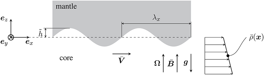
Figure 1. Schematic illustration of the core-mantle boundary region. Flow $\bar{\text{V}}$ of the core past the mantle is disturbed by topography h(x, y) on the core-mantle boundary. A stable density profile ρ(z) is assumed at the top of the core and a uniform vertical magnetic field $\bar{\text{B}}$ is imposed. Fluid motion perturbs the density profile and alters the magnetic field to produce a pressure field that exerts a net horizontal force on the mantle.

where $\tilde{h}$ is the amplitude, and k_x and k_y are the wavenumbers in the direction of the basis vectors e_x and e_y. A more general description of topography can be constructed from a linear superposition of sinusoidal components (Here we follow the convention of interpreting physical quantities as the real parts of complex expressions). The surface of the CMB is described by

$\begin{array}{cc}\begin{array}{r}f(x,y,z)=z-h(x,y)=0\end{array}& (2)\end{array}$

so the outward unit normal n to the fluid region is given by

$\begin{array}{cc}\begin{array}{r}\text{n}\equiv \frac{\nabla f}{|\nabla f|}=\frac{ez-\text{i}k\text{T}h(x,y)}{\sqrt{1+k_{\text{T}}^{2}Re{(\text{i}h)}^2}}\end{array}& (3)\end{array}$

where kT = k_xe_x + k_ye_y, k_T = |kT| and Re(•) denotes the real part. When the topography is small ($k_x\tilde{h}$ and $k_y\tilde{h}\ll 1$) we can set |∇f| ≈ 1 in the definition of n.

A uniform background flow $\bar{\text{V}}=\bar{V}ex$ is maintained in a frame that rotates with the mantle at constant angular velocity Ω = Ωe_z. The gravitational acceleration is g = −ge_z and we adopt a vertical background magnetic field $\bar{\text{B}}=\bar{B}ez$ because it has the largest influence on the dynamics once the flow is perturbed by boundary topography. We assume that the fluid is inviscid and the mantle is an electrical insulator, so the background magnetic field is not disturbed by $\bar{\text{V}}$ in the absence of topography. Thus the uniform (geostrophic) background flow is sustained by a horizontal pressure gradient $\nabla \bar{P}(y)$.

Stable stratification is imposed in the core by letting the density field vary linearly with depth

$\begin{array}{cc}\begin{array}{r}\bar{\rho }(z)={\rho }_0(1+\alpha z),\text{\hspace{1em} where }\alpha =\frac{1}{{\rho }_0}\frac{\partial \bar{\rho }}{\partial z}<0\end{array}& (4)\end{array}$

is required to ensure stable stratification in the region z < 0. We subsequently relate α to the buoyancy frequency N using α = −N²/g. Both α and N are treated as constants.

2.1. Linearized Governing Equations

Flow past topography alters the background flow and disturbs the magnetic field, pressure and density. We denote these perturbations using v for the velocity, b for the magnetic field, p for the pressure and ρ′ for the density. All of these fields are assumed to be small when the topography is small, so we can linearize the equations for the perturbations by neglecting products of small quantities. We expect these perturbations to become time invariant in the frame of the mantle after the passage of initial transients. Further simplifications are permitted by the low viscosity of the core liquid. Neglecting the viscous term in the linearized momentum equation yields

$\begin{array}{cc}\begin{array}{r}{\rho }_0\bar{\text{V}}·\nabla \text{v}+{\rho }_0\text{Ω}\times \text{v}=-\nabla p+{\rho }^{\prime }\text{g}+\frac{1}{\mu }\bar{\text{B}}·\nabla \text{b},\end{array}& (5)\end{array}$

where μ is the magnetic permeability. This particular form of the momentum equation accounts for the absence of a background electric current density, $\bar{\text{J}}=(\nabla \times \bar{\text{B}})/\mu =0$. The induction equation for a steady magnetic perturbation is

$\begin{array}{cc}\begin{array}{r}\bar{\text{B}}·\nabla \text{v}-\bar{\text{V}}·\nabla \text{b}+\eta {\nabla }^2\text{b}=\text{0},\end{array}& (6)\end{array}$

where η = 1/(μσ) is the magnetic diffusivity and σ is the electrical conductivity. Finally, conservation of mass requires

$\begin{array}{cc}\begin{array}{r}\bar{\text{V}}·\nabla {\rho }^{\prime }+\text{v}·\nabla \bar{\rho }=0.\end{array}& (7)\end{array}$

These three equations are supplemented by ∇ · b = 0, together with ∇ · v = 0 in the Boussinesq approximation.

Solutions for the perturbations are sought in the form

$\begin{array}{cc}\begin{array}{l}{\rho }^{\prime }={\tilde{\rho }}^{\prime }\exp (ik·x),v=\tilde{v}\exp (ik·x),\\ p=\tilde{p}\exp (ik·x),b=\tilde{b}\exp (ik·x),\end{array}& (8)\end{array}$

where k = k_xe_x + k_ye_y + k_ze_z is the wavenumber vector, x = xe_x + ye_y + ze_z is the position vector and ${\tilde{\rho }}^{\prime }$, $\tilde{\text{v}}$, etc. are the amplitude of the perturbations.

2.2. Boundary Conditions

Four boundary conditions are imposed at the CMB, in addition to the requirement that the perturbations vanish as z → −∞. An inviscid fluid requires a single boundary condition on the normal component of the total velocity

$\begin{array}{cc}\begin{array}{r}(\bar{\text{V}}+\text{v})·\text{n}=0.\end{array}& (9)\end{array}$

This condition is evaluated on the interface z = h(x, y), but it is customary to transfer the boundary condition to z = 0 by expanding $\bar{\text{V}}$ and v in Taylor series about the reference surface.

Three additional conditions are required to ensure that the magnetic perturbation in the core is continuous with the magnetic perturbation in the mantle, which can be represented as the gradient of a potential. A simpler treatment of the boundary condition on the magnetic field uses the so-called pseudo-vacuum condition (Jackson et al., 2014). In this case we have b_x = b_y = 0 at z = 0 to first-order in the perturbation. This approximation reduces the number of boundary conditions on the magnetic field from three to two, and eliminates the magnetic potential as an unknown in the problem. Even though both choices of magnetic boundary conditions yield quantitatively similar solutions (the relative difference in pressure is only 10-4) we adopt the potential-field condition

$\begin{array}{cc}\begin{array}{r}\begin{array}{ccccc}\hfill \text{b}(x,y,0)& ={\text{b}}_{\text{M}}(x,y,0)\hfill & \hfill & \mathrm{\text{with}}\hfill & \hfill {\text{b}}_{\text{M}}=-\nabla {\psi }_{\text{M}}(\text{x}).\end{array}\end{array}& (10)\end{array}$

for all solutions in this study. Here, b_M denotes the magnetic perturbation in the mantle and ψ_M is the associated scalar potential.

2.3. Solution for the Perturbation

In the Appendix, we show that Equations (5–7) can be reduced to a system of three linear equations for the amplitude of the magnetic perturbation $\tilde{\text{b}}$. Three independent solutions are found for $\tilde{\text{b}}$, each corresponding to a distinct value for the vertical wavenumber k_z. A linear combination of these three solutions are required to satisfy the boundary conditions at z = 0. For the case of a potential field in the mantle, we use four boundary conditions to determine the unknown amplitudes of the three solutions, as well as the amplitude of the magnetic potential. Once solutions are obtained for $k_z^{(i)}$ (i = 1, 2, 3), we use the linear combination of ṽ⁽ⁱ⁾ and ${\tilde{p}}^{(i)}$ to reconstruct the velocity and pressure perturbations everywhere in the fluid.

We adopt nominal values of the relevant parameters to illustrate the solution. We take the values specified in Table 1 to define the basic state of the core. A topography with a wavelength of 100 km in the e_x-direction yields the wave number stated in Table 1. The error due to omitted curvature terms is λ_x/R ≈ 0.03, which is small enough to neglect. The radial motion over this topography has a frequency $\omega =k_x\bar{V}=$3.1 × 10-8 s-1 for the background velocity chosen in Table 1, which corresponds to a timescale, 2π/ω, of roughly 6 years. We explore a range of values for the fluid stratification, starting with the case of strong stratification. Chemical stratification due to barodiffusion of light elements can produce a buoyancy frequency of N = 20Ω to 30Ω when the top of the core is not convectively mixed (Gubbins and Davies, 2013). Adopting N = 20Ω gives the following solution for the vertical wavenumbers:

$\begin{array}{cc}\begin{array}{lll}{k}_z^{(1)}& =& -1.56\times 10\text{-2}(1+\text{i})m\text{-1},k_z^{(2)}=1.40\times 10\text{-4}(1-\text{i})m\text{-1},\\ k_z^{(3)}& =& 5.42\times 10\text{-6}m\text{-1}.\end{array}& (11)\end{array}$

TABLE 1

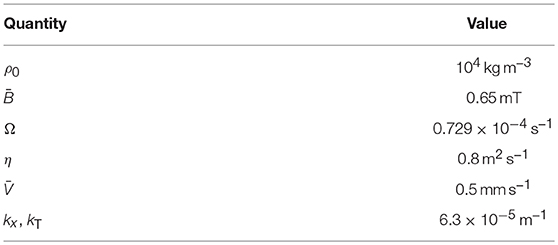
Table 1. Nominal values for the parameters of the model.

The first wave can be interpreted as a boundary-layer solution due to the short length scale in the vertical direction. The vertical length scale for this particular solution is dependent on the strength of stratification. We find that $k_z^{(1)}$ increases linearly with N, so the strongest stratification produces the thinnest boundary layer. The second wave has a larger vertical length scale, comparable to the wavelength of topography. The third wave has a much larger vertical length scale with a very small imaginary part due to the weak influence of magnetic diffusion at these larger scales. The first and third waves contribute most to the pressure field for our nominal values; the first wave sets the pressure at the boundary, and the third wave controls the broader background perturbation well below the boundary.

Figure 2 shows a vertical x-z cross-section for the pressure field using the nominal parameter values and a topography of $\tilde{h}=30m$. The pressure immediately adjacent to the boundary is asymmetric with respect to the topography. High pressure occurs mostly over the leading edge of the bump on the boundary, while low pressure prevails over the trailing edge. Both of these pressure perturbations exert a horizontal (tangential) stress on the boundary. A quantitative estimate for the average tangential stress is obtained by integrating the local traction over the surface of the CMB. Before turning to this question we assess the importance of stratification for producing an observable tangential stress. When the stratification is substantially reduced (say N = 0.1Ω) the thickness of the boundary-layer solution (first wave) increases and the resulting contribution to the pressure at the CMB is small. The second and third wave now contribute most to pressure perturbation. However, the distribution of pressure is symmetric relative to the topography, so the average tangential stress is vanishingly small.

FIGURE 2

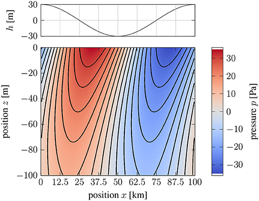
Figure 2. Vertical cross-section of pressure perturbation relative to the boundary topography. A positive pressure perturbation develops over the leading edge of topography and a negative pressure perturbation occurs over the trailing edge. The disturbance in the flow is confined to the top kilometer of the core for the nominal choice of model parameters (see text).

The velocity perturbation on a x-z cross-section is shown in Figure 3. Flow over the topography causes a vertical component of flow, but the magnitude of this flow is quite small relative to the horizontal flow. The peak vertical velocity is only 0.001 mm s-1 because the slope of the topography is very small (e.g., $k_x\tilde{h}\ll 1$). The largest horizontal flow occurs immediately below the CMB and it decays rapidly with depth. The peak horizontal velocity is 0.3 mm s-1, which is less than the background flow of 0.5 mm s-1, although not substantially less. A large velocity perturbation means that the linearized equations are less accurate. We revisit this question qualitatively in the discussion, but a more quantitative assessment must retain the nonlinear terms in the governing equations. We could reduce the velocity perturbation by reducing the topography. While this change would improve the validity of the linearized equations, it would also reduce the traction on the boundary. We show in the next section that the choice of $\tilde{h}=30m$ is sufficient to produce a torque on the mantle of roughly 1019 N m. Such a torque is probably more than enough to account for the LOD variations, although it does suggest that the flow is becoming nonlinear as we approach the conditions required to explain the observations.

FIGURE 3

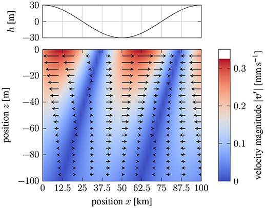
Figure 3. Vertical cross-section of horizontal velocity relative to the boundary topography. Arrows show the direction of flow and background color denotes the magnitude of the flow. Negative velocity perturbations under regions of positive topography implies that the total flow is decreasing.

Information about the nature of the nonlinearity can be gleaned from Figure 3. For example, the velocity perturbation on the leading side of the topography (x ≈ 0 km to 20 km) is directed in the negative e_x direction. This means that the total velocity, $\overline{V}+v$, in this region is decreasing. In effect, the fluid is becoming stagnant below regions of positive topography. This stagnant fluid prevents flow from following the boundary, reducing the forcing of vertical motion and lowering the amplitude of the perturbation. We might view the growth of stagnant regions as a reduction in the effective topography. We speculate that increasing stratification or increasing topography would cause the flow to become increasingly stagnant below positive topography. Deeper flow would be unimpeded by the topography, so magnetic stresses on the shallower stagnant fluid would transfer momentum to the mantle by the effects of pressure on the boundary. Such a coupling mechanism is qualitatively similar to electromagnetic coupling, where the thickness of the conducting layer is set by the amplitude of the topography. A topography of $\tilde{h}=$100 m would approximate a conducting layer with a conductance of G = hσ = 108 S, when the electrical conductivity is σ = 106 S m-1. This is the conductance required to account for LOD variations (Holme, 1998). Thus, we expect nonlinearities to reduce the effectiveness of the coupling mechanism. However, we can compensated by increasing the amplitude of the topography above the nominal value of $\tilde{h}=$30 m.

3. Average Tangential Stress on the Boundary

The local traction on the mantle is

$\begin{array}{cc}\begin{array}{r}\text{t}=p(x,y,0)\text{n},\end{array}& (12)\end{array}$

where n was previously defined in Equation (3) as the outward normal to the core. In general we can expect t to have both e_x and e_y components when the wavenumbers k_x and k_y are non-zero. Setting k_y = 0 produces topographic ridges that are perpendicular to the background flow, so the horizontal traction is entirely in the e_x direction. A local traction in the e_x direction also occurs for a linear superposition of topography with wavenumbers kT = k_xe_x ± k_ye_y. This particular choice of topography produces a checkerboard pattern of relief on the boundary, but it gives no net traction perpendicular to the direction of background flow. For the purpose of illustration, we consider the simple case where k_x = k_T and k_y = 0, so we confine our attention to tractions in the direction of flow.

Transfer of angular momentum to the mantle depends on the average of t_x over x. We compute the average traction from the real part of t_x in Equation (12), noting that Re(p) = (p+p*)/2, where (•)* denotes the complex conjugate. Similarly, we let Re(n) = (n + n*)/2. Only constant terms in the product pn contribute to the average stress, so we obtain:

$\begin{array}{cc}\begin{array}{r}\langle t_x\rangle =\frac{1}{4}(p{n}_x^{*}+p^{*}{n}_x).\end{array}& (13)\end{array}$

For our representative parameters values we obtain an average stress of 0.027 N m-2, which is comparable to the estimate required to account for fluctuations in LOD at periods of several decades (Hide, 1969). A rough estimate for the axial torque due to zonal flow with constant $\bar{V}$ is ${\pi }^2{R}^3\langle t_x\rangle$, where R = 3, 480 km is the radius of the core (details are given below). Thus the nominal value for the average stress predicts an axial torque of about 1.1 × 1019 N m.

Many of the parameters in 〈t_x〉 are uncertain, so it is useful to consider a range of possible parameter values. Figure 4 shows how 〈t_x〉 changes when a selected parameter is varied. In each case the other parameters are fixed at their nominal values. We consider variations in $\tilde{h}$, N, $\bar{V}$, Ω, and λ_x. The strongest dependence is due to topography $\tilde{h}$. Because p and n_x depend linearly on $\tilde{h}$, the product for the average stress varies as ${\tilde{h}}^2$. Increasing the topography to 100 m produces a tangential stress of 0.3 N m-2, which is much larger than the value required to account for LOD fluctuations. Independent estimates of boundary topography can exceed several kilometers (Colombi et al., 2014; Shen et al., 2016), although the corresponding wavelengths are comparable to the radius of the core. Increasing the wavelength from 100 km to 1,000 km decreases the magnitude of the stress to 0.02 N m-2 for $\tilde{h}=30m$. Restoring the stress to our nominal value of 0.027 N m-2 requires a modest increase in the topography to $\tilde{h}=42m$. Wavelengths larger than 1,000 km would likely require an explicit treatment of spherical geometry (Anufriyev and Braginski, 1977).

FIGURE 4

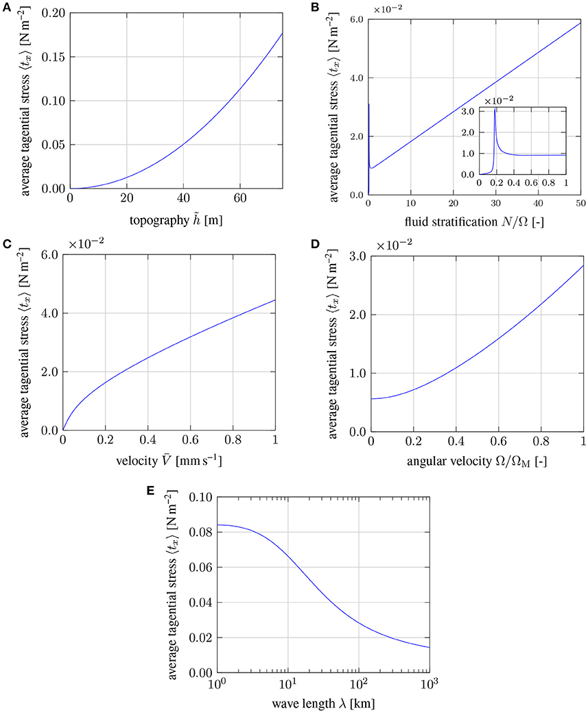
Figure 4. Dependence of the tangential stress 〈t_x〉 on (A) the amplitude of topography $\tilde{h}$, (B) the strength of stratification N/Ω, (C) on the velocity $\bar{V}$, (D) on the angular velocity Ω, and (E) the wavelength of topography λ = 2π/k.

Stratification is essential for producing a tangential traction. We find that 〈t_x〉 varies linearly with N over a large range of stratifications (see Figure 4B). A resonance is evident at low N (see the inset in Figure 4B), possibly due to a correspondence between the frequency of the boundary forcing and the natural frequency of internal gravity waves. Further reductions in stratification causes the average stress drop to zero. A wide range of values for N can sustain a viable coupling mechanism. Decreasing stratification to N = Ω lowers the stress to roughly 〈t_x〉 = 0.01 N m, although we can restore the stress to 0.027 N m-1 with a modest increase in the topography to $\tilde{h}=52m$ (The peak amplitude of the perturbed flow is still 0.3 mm s-1). Thus an intermediate stratification of N≈Ω, as reported in previous studies of geomagnetic secular variation (Buffett et al., 2016), is compatible with the coupling mechanism proposed here.

A broad (140 km) layer of stratification would allow barodiffusion to drive a flux of light elements toward the CMB. As light elements accumulate at the top of the core we can expect a 1 km layer of chemical stratification to develop within a few million years, given typical estimates for the diffusivity of light elements (Pozzo et al., 2012). A buoyancy frequency of N = 20Ω or more is feasible due to chemical stratification, which would put the core at the high end of stratifications considered in Figure 4. While it is not entirely clear how a thin layer of stratification would affect the average stress, we note that the perturbed flow due to the first wave would be largely contained within the chemical stratification. Recall that the first wave was principally responsible for the average boundary stress, so it is at least possible for a thin layer of stratification to be relevant for core-mantle coupling.

The amplitude of the background flow also affects the average tangential stress. Figure 4C shows that 〈t_x〉 varies at ${\bar{V}}^{1/2}$. This implies a relatively weak dependence on the background velocity. If the amplitude of the velocity variations associated to LOD fluctuations is roughly an order of magnitude smaller than 0.5 mm s-1, this would lower the fluctuating stress by a factor of 3. The strong dependence on $\tilde{h}$ means that only a modest increase in topography would be required to restore our nominal estimate for the stress. A nonlinear dependence of the stress on $\bar{V}$ also has interesting consequences for the nature of the coupling mechanism, which may produce detectable signatures in the frequency spectra of LOD variations. We explore this behavior in the next section.

One other feature of the solution for 〈t_x〉 should be noted. We have assumed that the rotation vector Ω is perpendicular to the surface. This is strictly true in polar regions. Elsewhere we might interpret Ω as the radial component of the planetary rotation rate. This is a common assumption when the flow is confined to a thin layer (Pedlosky, 1987, p. 715). Our boundary-layer solution (first wave) is confined to a thin layer, so it might be reasonable to replace the value of planetary rotation with the radial component at mid-latitudes, which would imply a 30 % reduction in the value of Ω. A direct calculation of 〈t_x〉 with the lower rotation rate is shown in Figure 4D. The average stress is found to vary quadratically with Ω, although the stress does not go to zero when the rotation rate vanishes. We use this result below to estimate the torque due to the boundary stress. To simplify the calculation of the torque we adopt a linear approximation for the average stress. It gives good agreement at mid to high latitudes (e.g., 0.7Ω to Ω), but underestimates the stress at the equator, where the usual assumption about retaining only the radial component of the rotation vector break down. It is likely that this approximation underestimates the torque on the mantle.

3.1. Torque Due to Boundary Stress

The axial torque on the mantle is evaluated using local estimates for 〈t_x〉 over the surface of the CMB. A detailed assessment should account for changes in the radial component of planetary rotation by letting Ω = ΩMantlecos(θ), where ΩMantle is the angular velocity of the mantle and θ is the colatitude. We also require knowledge of the zonal (eastward) flow of the core $\bar{\text{V}}=\bar{V}e\phi$ relative to the mantle. Here eφ denotes the unit vector in the azimuthal direction. As a first approximation, we might define the relative motion of the core in terms of an average angular velocity of the core ΩCore. Thus the relative motion can be expressed in the form

$\begin{array}{cc}\begin{array}{r}\bar{V}=R({\text{Ω}}_{\text{C}}-{\text{Ω}}_{\text{M}})sin(\theta ).\end{array}& (14)\end{array}$

Variations in $\bar{V}$ cause changes in 〈t_x〉, so we might define the average tangential stress (now defined in the eφ direction) in the form

$\begin{array}{cc}\begin{array}{r}\langle t_{\phi }\rangle =t_{\phi ,0}cos(\theta )\sqrt{\frac{R({\Omega }_{\text{C}}-{\Omega }_{\text{M}})sin(\theta )}{{\bar{V}}_0}}\end{array}& (15)\end{array}$

where t_{φ, 0} represents the nominal value for the average stress due to the nominal background velocity ${\bar{V}}_0$. If we set $\bar{V}={\bar{V}}_0$ at a particular co-latitude, θ, then the average stress at this location deviates from our nominal value, t_{φ, 0}, only due to the change in the radial component of Ω_M. However, if $\bar{V}$ also deviates from ${\bar{V}}_0$ then we want to account for the ${\bar{V}}^{1/2}$ dependence of the stress. For the purpose of illustration we let ${\bar{V}}_0=R(\Omega Core-\Omega Mantle)$, so the nominal background velocity occurs at the equator. Elsewhere the background velocity from Equation (14) is lower than ${\bar{V}}_0$. The resulting axial component of the torque on the mantle is given by

$\begin{array}{cc}\begin{array}{r}{\text{Γ}}_z={\displaystyle \underset{S}{\int }}ez·(\text{r}\times \langle t_{\phi }\rangle e\phi )\text{d}S=t_{\phi ,0}{\displaystyle \underset{S}{\int }}Rcos(\theta ){sin}^{\frac{3}{2}}(\theta )\text{d}S=\frac{8\pi }{7}{R}^3{t}_{\phi ,0}\end{array}& (16)\end{array}$

where r is the position vector relative to the center of the planet and S defines the surface of the CMB. The stress is symmetric about the equator, even though the direction of the Coriolis force changes sign in the Southern Hemisphere. Consequently, we restrict the surface integral to the North Hemisphere and exploit the symmetry to evaluate Γ_z. The net torque is about a factor of 3 lower than our earlier approximation because the background flow and rotation rate are lower over most of the CMB.

3.2. Dynamics of the Core-Mantle System

The weak (square-root) dependence of the average stress on the background velocity has several consequences for the transfer of angular momentum. Consider the case where Ω_C > Ω_M. According to Equation (16) the torque on the mantle is positive, while the torque on the core is negative. The negative torque on the core causes a decrease in Ω_C, which reduces the differential rotation. The angular velocity of the mantle is also altered, but this change is smaller due to the larger moment of inertia. For the hypothetical case of a torque that depends linearly on the differential rotation, the relaxation back to solid-body rotation occurs exponentially with time. By comparison, a square-root dependence of the torque on Ω_C − Ω_M means that the torque is smaller at large differential rotations; the initial adjustment occurs more slowly than the linear torque. However, at sufficiently small differential rotation the torque in Equation (16) must exceed the torque with a linear dependence on Ω_C − Ω_M. The larger torque drives the differential rotation to zero in finite time (unlike exponential decay).

Signatures of the coupling mechanism are potentially detectable in the dynamics of the core-mantle system. To explore this question we consider a toy problem in which the mantle is forced by an atmospheric torque ΓAtmos(t) with a period of one cycle per year (cpy). The actual problem is more complicated (Gross et al., 2004), but the goal here is to assess the influence of different functional forms for the torque at the CMB. When there are no other torques on the core, we can write the coupled system of angular momentum equations in the form

$\begin{array}{cc}\begin{array}{rc}{\text{C}}_{\text{M}}\frac{{\text{dΩ}}_{\text{M}}}{\text{d}t}& =\gamma sgn({\text{Ω}}_{\text{C}}-{\text{Ω}}_{\text{M}})\sqrt{|{\text{Ω}}_{\text{C}}-{\text{Ω}}_{\text{M}}|}+\text{Γ}A(t),\end{array}& (17)\end{array}$

$\begin{array}{cc}\begin{array}{rc}{\text{C}}_{\text{C}}\frac{{\text{dΩ}}_C}{\text{d}t}& =-\gamma sgn({\text{Ω}}_{\text{C}}-{\text{Ω}}_{\text{M}})\sqrt{|{\text{Ω}}_{\text{C}}-{\text{Ω}}_{\text{M}}|},\end{array}& (18)\end{array}$

where C_M and C_C are the polar moments of inertia of the mantle and core, γ characterizes the amplitude of core-mantle coupling and sgn(•) defines the sign of the torque according to the sign of the argument; the square-root dependence is applied to the absolute value of Ω_C − Ω_M. The moment of inertia of the mantle is about a factor of 10 larger than the moment of inertia of the core. Similarly, the atmospheric torque might be roughly 50 times larger than the torque at the CMB. We approximate these conditions by defining Γ_A(t) with unit amplitude and take CM = 1 kg m2, CC = 0.1 kg m2, and γ = 0.02 N m s1/2. We also consider a case in which core-mantle coupling is turned off (γ = 0). These results are compared with a third solution in which the torque at the CMB depends linearly on Ω_C−Ω_M. Each of these systems are integrated numerically in time using a solid-body rotation as the initial condition, i.e., Ω_M(0) = Ω_C(0) = Ω₀, where Ω₀ is the initial rate of rotation.

Figure 5 shows the power spectrum computed from the numerical solution for Ω_M(t). The solution with no coupling at the core-mantle boundary produces a single spectral peak at the frequency of the atmospheric torque. The spectrum produced with the linear coupling mechanism is indistinguishable from the one with γ = 0 and therefore not shown. This result indicates that the core has a small influence on the response of the mantle to atmospheric forcing. The coupling mechanism with nonlinear (square-root) dependence also reproduces the peak at 1 cpy, but adds several other peaks at 3, 5, 7, …cpy. These peaks are simply a consequence of the specific form of the nonlinearity in the coupling mechanism.

FIGURE 5

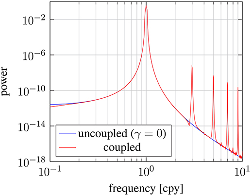
Figure 5. Power spectra for the angular velocity of the mantle Ω_M(t) in response to an imposed annual torque from the atmosphere. A reference model with no coupling to the core (γ = 0) is compared to a nonlinear model, based on the horizontal boundary stress 〈t_φ〉. The two results are nearly identical at the forcing frequency of 1 cycle per year, whereas the nonlinear model exhibits overtones due to the nonlinearity of the coupling mechanism. Low-amplitude fluctuations near the base of the spectra are a result of discretization errors in the numerical integration of Ω_M(t).

4. Discussion

The coupling mechanism proposed here involves a combination of pressure and electromagnetic forces. Momentum is transferred to the mantle by the influence of pressure on topography. However, the distribution of pressure over the boundary is strongly influenced by stratification and by electromagnetic forces. In fact, the coupling mechanism can be as dissipative as electromagnetic coupling. Steep gradients in the perturbed flow distort the radial magnetic field over a length scale of roughly 102 m to 103 m, depending on the strength of the stratification. This length scale is short compared with the skin depth, based on the temporal frequency of flow over the topography. Pervasive diffusion of the magnetic perturbation occurs in a magnetic boundary-layer (i.e., the first wave).

Other components of the background magnetic field can also contribute to the coupling mechanism, although they would likely have a smaller role. Distortion of a horizontal background magnetic field is due to lateral variations in the flow, which is controlled by the wavelength of topography. This length scale is typically long compared with the vertical wavelength. The study of Moffatt (1977) dealt exclusively with the influence of a horizontal magnetic field on flow over topography (in the absence of stratification) and found that topography in excess of 4 km was required to produce a stress comparable to our nominal value of 0.027 N m-2. By comparison, much smaller boundary topographies are sufficient to account for the amplitude of decadal fluctuations in LOD when we allow for fluid stratification. A small topography is also consistency with our method of solution because we use a Taylor series to transfer boundary conditions to the reference surface z = 0. When the boundary topography is small compared with the vertical length scale of the perturbation, a first-order Taylor series suffices to relate the conditions on z = h(x, y) to those on z = 0.

The amplitude of the topography is also important for determining the amplitude of the velocity perturbation. A nominal topography of $\tilde{h}=30m$ in Figure 3 produces a maximum velocity of 0.3 mm s-1 at the CMB (see Figure 3). Thus the perturbed flow is not substantially smaller than the background flow of 0.5 mm s-1. We expect nonlinearities to reduce the effectiveness of the coupling mechanism, so a modest increase topography above the nominal value of $\tilde{h}=30m$ is probably required to compensate. Our calculations show that disturbance in the background flow is confined to the top 100 m of the core. Such a shallow disturbance may not substantially alter the influence of deeper background flow on geomagnetic secular variation (It would be analogous to diffusing the geomagnetic field through a thin conducting layer). We also expect the vertical (radial) component of the magnetic perturbation to be small, so it would be difficult to detect at the surface, particularly if the wavelength of topography was on the order of 102 km. Other aspects of the dynamics could more significant. Enabling an effective means of momentum transfer alters the structure of waves in the core and may also account for the damping of torsional waves in the equatorial region (Gillet et al., 2010). Electromagnetic coupling has been proposed as a damping mechanism for torsional waves (Schaeffer and Jault, 2016), but the mechanism proposed here may work similarly without requiring a large electrical conductivity on the mantle-side of the boundary. A suitably modification of the proposed mechanism is also applicable to tidally driven flow in the core (Buffett, 2010). Observations of Earth's nutation require a source of dissipation at the CMB. Electromagnetic coupling is one interpretation, but the influence of topography in the presence of stratification offers an alternative explanation.

5. Conclusions

Steady flow of Earth's core over boundary topography can produce a large tangential stress on the mantle when the top of the core is stably stratified. This stress provides an effective means of transferring angular momentum across the CMB. A linearized model is developed using a planar approximation of the CMB. Topography on the boundary disturbs the velocity and magnetic fields, causing a pressure perturbation that exerts a net horizontal force on topographic features. Reasonable choices for the amplitude of the background flow and the strength of the initial magnetic field yield dynamically significant stresses on the mantle. A viable solution has a topography of 52 m and a fluid stratification specified by N≈Ω. Stronger stratification, possibly due to a thin layer of chemical stratification, increases the stress in proportion to the value of N and lowers the required topography. We also show that the stress has a quadratic dependence on the amplitude of topography, but varies more weakly with the square root of the fluid velocity. Incorporating this coupling mechanism into a simple model for angular momentum exchange yields a nonlinear system of equations, which produces odd overtones in the response to annual forcing by an imposed torque from the atmosphere. Spectral properties of the resulting changes in LOD may offer insights into the underlying coupling mechanisms.

Author Contributions

BB proposed the project and SG carried out the analysis. Both authors contributed to the writing of the paper.

Funding

This work is partially supported by the National Science Foundation (grant EAR-1430526).

Conflict of Interest Statement

The authors declare that the research was conducted in the absence of any commercial or financial relationships that could be construed as a potential conflict of interest.

Supplementary Material

The Supplementary Material for this article can be found online at: https://www.frontiersin.org/articles/10.3389/feart.2018.00171/full#supplementary-material

References

Amit, H. (2014). Can downwelling at the top of the earth's core be detected in the geomagnetic secular variation? Phys. Earth Planet. Inter. 229, 110–121. doi: 10.1016/j.pepi.2014.01.012

CrossRef Full Text | Google Scholar

Anufriyev, A. P., and Braginski, S. I. (1977). Effect of irregularities of the boundary of the earth's core on the speed of the fluid flow and on the magnetic field, iii. Geomag. Aeron. 17, 492–496.

Google Scholar

Bloxham, J. (1986). The expulsion of magnetic flux from the earth's core. Geophys. J. Int. 87, 669–678. doi: 10.1111/j.1365-246X.1986.tb06643.x

CrossRef Full Text | Google Scholar

Bloxham, J. (1990). On the consequences of strong stable stratification at the top of earth's outer core. Geophys. Res. Lett. 17, 2081–2084. doi: 10.1029/GL017i012p02081

CrossRef Full Text | Google Scholar

Braginsky, S. I. (1993). MAC-oscillations of the hidden ocean of the core. J. Geomagn. Geoelectr. 45, 1517–1538. doi: 10.5636/jgg.45.1517

CrossRef Full Text | Google Scholar

Buffett, B. A. (1996). Gravitational oscillations in the length of day. Geophys. Res. Lett. 23, 2279–2282. doi: 10.1029/96GL02083

CrossRef Full Text | Google Scholar

Buffett, B. A. (2010). Chemical stratification at the top of earth's core: constraints from observations of nutations. Earth Planet. Sci. Lett. 296, 367–372. doi: 10.1016/j.epsl.2010.05.020

CrossRef Full Text | Google Scholar

Buffett, B. A. (2014). Geomagnetic fluctuations reveal stable stratification at the top of the earth's core. Nature 507, 484–487. doi: 10.1038/nature13122

PubMed Abstract | CrossRef Full Text | Google Scholar

Buffett, B. A., Garnero, E. J., and Jeanloz, R. (2000). Sediments at the top of Earth's core. Science 290, 1338–1342. doi: 10.1126/science.290.5495.1338

PubMed Abstract | CrossRef Full Text | Google Scholar

Buffett, B. A., Knezek, N., and Holme, R. (2016). Evidence for MAC waves at the top of Earth's core and implications for variations in length of day. Geophys. J. Int. 204, 1789–1800. doi: 10.1093/gji/ggv552

CrossRef Full Text | Google Scholar

Bullard, E. C., Freeman, C., Gellman, H., and Jo, N. (1950). The westward drift of the earth's magnetic field. Philos. Trans. R. Soc. 243, 67–92. doi: 10.1098/rsta.1950.0014

CrossRef Full Text | Google Scholar

Christensen, U. R. (2018). Geodynamo models with a stable layer and heterogeneous heat flow at the top of the core. Geophys. J. Int. 215, 1338–1351. doi: 10.1093/gji/ggy352

CrossRef Full Text | Google Scholar

Christensen, U. R., Aubert, J., and Hulot, G. (2010). Conditions for Earth-like geodynamo models. Earth Planet. Sci. Lett. 296, 487–496. doi: 10.1016/j.epsl.2010.06.009

CrossRef Full Text | Google Scholar

Colombi, A., Nissen-Meyer, T., Boschi, L., and Giardini, D. (2014). Seismic waveform inversion for core–mantle boundary topography. Geophys. J. Int. 198, 55–71. doi: 10.1093/gji/ggu112

CrossRef Full Text | Google Scholar

Gill, A. E. (1982). Atmosphere-Ocean Dynamics Vol. 30 of International Geophysics Series, 1st Edn. San Diego, CA: Academic Press.

Google Scholar

Gillet, N., Jault, D., Canet, E., and Fournier, A. (2010). Fast torsional waves and strong magnetic field within the Earth's core. Nature 465, 74–77. doi: 10.1038/nature09010

PubMed Abstract | CrossRef Full Text | Google Scholar

Gillet, N., Pais, M. A., and Jault, D. (2009). “Ensemble inversion of time-dependent core flow models.” Geochem. Geophys. Geosys. 10:Q06004. doi: 10.1029/2008GC002290

CrossRef Full Text | Google Scholar

Gross, R. S. (2015). “Chapter 9: Earth rotation variations – long period,” in Treatise on Geophysics, Vol. 3, 2nd Edn, ed G. Schubert (Oxford: Elsevier), 215–261.

Google Scholar

Gross, R. S., Fukumori, I., Menemenlis, D., and Gegout, P. (2004). Atmospheric and oceanic excitation of length-of-day variations during 1980–2000. J. Geophys. Res. 109:B01406. doi: 10.1029/2003JB002432

CrossRef Full Text | Google Scholar

Gubbins, D. (2007). Geomagnetic constraints on stratification at the top of earth's core. Earth Planets Space 59, 661–664. doi: 10.1186/BF03352728

CrossRef Full Text | Google Scholar

Gubbins, D., and Davies, C. J. (2013). The stratified layer at the core-mantle boundary caused by barodiffusion of oxygen, sulphur and silicon. Phys. Earth Planet. Inter. 215, 21–28. doi: 10.1016/j.pepi.2012.11.001

CrossRef Full Text | Google Scholar

Hide, R. (1969). Interaction between the Earth's Liquid Core and Solid Mantle. Nature 222, 1055–1056. doi: 10.1038/2221055a0

CrossRef Full Text | Google Scholar

Holme, R. (1998). Electromagnetic core—mantle coupling—I. Explaining decadal changes in the length of day. Geophys. J. Int. 132, 167–180. doi: 10.1046/j.1365-246x.1998.00424.x

CrossRef Full Text | Google Scholar

Jackson, A., Jonkers, A. R. T., and Walker, M. R. (2000). Four centuries of geomagnetic secular variation from historical records. Philos. Trans. R. Soc. Lond. A 358, 957–990. doi: 10.1098/rsta.2000.0569

CrossRef Full Text | Google Scholar

Jackson, A., Sheyko, A., Marti, P., Tilgner, A., Cébron, D., Vantieghem, S., et al. (2014). A spherical shell numerical dynamo benchmark with pseudo-vacuum magnetic boundary conditions. Geophys. J. Int. 196, 712–723. doi: 10.1093/gji/ggt425

CrossRef Full Text | Google Scholar

Jault, D. (2008). Axial invariance of rapidly varying diffusionless motions in the earth's core interior. Phys. Earth Planet. Inter. 166, 67–76. doi: 10.1016/j.pepi.2007.11.001

CrossRef Full Text | Google Scholar

Jault, D., and Finlay, C. (2015). “Chapter 9: Waves in the core and mechanical core–mantle interactions,” in Treatise on Geophysics, Vol. 8, 2nd Edn., ed G. Schubert (Oxford: Elsevier), 225–244.

Google Scholar

Jault, D., Gire, C., and Le Mouel, J. L. (1988). Westward drift, core motions and exchanges of angular momentum between core and mantle. Nature 333, 353–356. doi: 10.1038/333353a0

CrossRef Full Text | Google Scholar

Jones, C. A. (2011). Planetary magnetic fields and fluid dynamos. Annu. Rev. Fluid Mech. 43, 583–614. doi: 10.1146/annurev-fluid-122109-160727

CrossRef Full Text | Google Scholar

Kanda, R. V. S., and Stevenson, D. J. (2006). Suction mechanism for iron entrainment into the lower mantle. Geophys. Res. Lett. 33:L02310. doi: 10.1029/2005GL025009

CrossRef Full Text | Google Scholar

Lay, T., Williams, Q., and Garnero, E. J. (1998). The core-mantle boundary layer and deep earth dynamics. Nature 392, 461–468. doi: 10.1038/33083

CrossRef Full Text | Google Scholar

Lesur, V., Whaler, K., and Wardinski, I. (2015). Are geomagnetic data consistent with stably stratified flow at the core-mantle boundary? Geophys. J. Int. 201, 929–946. doi: 10.1093/gji/ggv031

CrossRef Full Text | Google Scholar

Miller, K. J., Montési, L. G., and Zhu, W. -l. (2015). Estimates of olivine-basaltic melt electrical conductivity using a digital rock physics approach. Earth Planet. Sci. Lett. 432, 332–341. doi: 10.1016/j.epsl.2015.10.004

CrossRef Full Text | Google Scholar

Moffatt, H. K. (1977). Topographic coupling at the core-mantle interface. Geophys. Astrophys. Fluid Dyn. 9, 279–288. doi: 10.1080/03091927708242332

CrossRef Full Text | Google Scholar

More, C., and Dumberry, M. (2018). Convectively driven decadal zonal accelerations in earth's fluid core. Geophys. J. Int. 213, 434–446. doi: 10.1093/gji/ggx548

CrossRef Full Text | Google Scholar

Mound, J. E., and Buffett, B. A. (2005). Mechanisms of core-mantle angular momentum exchange and the observed spectral properties of torsional oscillations. J. Geophys. Res. 110:B08103. doi: 10.1029/2004JB003555

CrossRef Full Text | Google Scholar

Ohta, K., Hirose, K., Ichiki, M., Shimizu, K., Sata, N., and Ohishi, Y. (2010). Electrical conductivities of pyrolitic mantle and morb materials up to the lowermost mantle conditions. Earth Planet. Sc. Lett. 289, 497–502. doi: 10.1016/j.epsl.2009.11.042

CrossRef Full Text | Google Scholar

Olson, P., Landeau, M., and Reynolds, E. (2017). Dynamo tests for stratification below the core-mantle boundary. Phys. Earth Planet. Inter. 271, 1–18. doi: 10.1016/j.pepi.2017.07.003

CrossRef Full Text | Google Scholar

Otsuka, K., and Karato, S. (2012). Deep penetration of molten iron into the mantle caused by a morphological instability. Nature 492, 243–246. doi: 10.1038/nature11663

PubMed Abstract | CrossRef Full Text | Google Scholar

Pedlosky, J. (1987). Geophysical Fluid Dynamics, 2nd Edn. New York, NY: Springer.

Google Scholar

Pozzo, M., Davies, C., Gubbins, D., and Alfè, D. (2012). Thermal and electrical conductivity of iron at earth's core conditions. Nature 485, 355–358. doi: 10.1038/nature11031

PubMed Abstract | CrossRef Full Text | Google Scholar

Rochester, M. G. (1962). Geomagnetic core-mantle coupling. J. Geophys. Res. 67, 4833–4836. doi: 10.1029/JZ067i012p04833

CrossRef Full Text | Google Scholar

Schaeffer, N., and Jault, D. (2016). Electrical conductivity of the lowermost mantle explains absorption of core torsional waves at the equator. Geophys. Res. Lett. 43, 4922–4928. doi: 10.1002/2016GL068301

CrossRef Full Text | Google Scholar

Shen, Z., Ni, S., Wu, W., and Sun, D. (2016). Short period ScP phase amplitude calculations for core-mantle boundary with intermediate scale topography. Phys. Earth Planet. Inter. 253, 64–73. doi: 10.1016/j.pepi.2016.02.002

CrossRef Full Text | Google Scholar

Sreenivasan, B., and Gubbins, D. (2008). Dynamos with weakly convecting outer layers: implications for core-mantle boundary interaction. Geophys. Astrophys. Fluid Dyn. 102, 395–407. doi: 10.1080/03091920801900047

CrossRef Full Text | Google Scholar

Stevenson, D. J. (1987). Limits on lateral density and velocity variations in the earth's outer core. Geophys. J. R. Astron. Soc. 88, 311–319. doi: 10.1111/j.1365-246X.1987.tb01383.x

CrossRef Full Text | Google Scholar

Wardinski, I., and Lesur, V. (2012). An extended version of the C³FM geomagnetic field model: application of a continuous frozen-flux constraint. Geophys. J. Int. 189, 1409–1429. doi: 10.1111/j.1365-246X.2012.05384.x

CrossRef Full Text | Google Scholar

Wicks, J. K., Jackson, J. M., and Sturhahn, W. (2010). Very low sound velocities in iron-rich (Mg,Fe)O: implications for the core-mantle boundary region. Geophys. Res. Lett. 37:L15304. doi: 10.1029/2010GL043689

CrossRef Full Text | Google Scholar