The Definition of Bioregions in Palaeontological Studies of Diversity and Biogeography Affects Interpretations: Palaeozoic Tetrapods as a Case Study

Introduction

Ever since the seminal paper of Whittaker (1960), diversity has been discussed in terms of alpha, beta and gamma diversity. Gamma diversity (the total species richness of an assemblage or time bin) is a function of the species richness within each locality or habitat, or to use a more general term, “Bioregion” (alpha diversity), and the taxonomic differentiation between the bioregions (beta diversity).

When assessing either regional species richness or beta diversity, the definition of the bioregions can have a substantial effect on the results (Hausdorf, 2002; Ferrari, 2017). Unfortunately, the definition of bioregions in palaeontological studies of historical biogeography, beta diversity and regional species richness has been inconsistent and often extremely arbitrary. A wide range of scales has been employed, ranging from individual localities (Sahney et al., 2010; Vavrek and Larsson, 2010), to formations/basins (Sidor et al., 2013) to environmental/climatic zones (Sepkoski, 1988; Tougard, 2001; Qian and Ricklefs, 2007; Brocklehurst et al., 2017) to continents (Murray, 2001; Upchurch et al., 2002; Allwood et al., 2010; Benson et al., 2013, 2016; Upchurch P. et al., 2015; Dunhill et al., 2016; Silvestro et al., 2016). More recently, Button et al. (2017) attempted to remove the subjectivity, grouping localities based on their palaeocoordinates using k-means clustering. While less arbitrary, the bioregions resulting will be based on the spread and density of sampling rather than any biologically meaningful criteria.

The lack of a general framework for defining bioregions in paleontology has greater issues than simply their subjective nature. Not only are the results obtained when analyzing biogeographic patterns at such vastly different scales unlikely to be directly comparable (Welsh, 1994), but spatial patterns of diversity will be different at different scales (Palmer and White, 1994; Rosenweig, 1995; Whittaker et al., 2001; Field et al., 2009; Keil et al., 2012). Moreover, the spatial scale at which particular patterns are observed will be specific to the taxon of interest, influenced by size and dispersal capacity (Keil et al., 2012; Barton et al., 2013).

An illustration of how different definitions of bioregions can affect the results is provided by recent research into the biogeographic patterns in Palaeozoic tetrapods. Dunne et al. (2018) and Brocklehurst et al. (2018a) used different methods to examine changes in faunal provinciality and dispersal patterns and found conflicting signals across the Carboniferous/Permian boundary. Brocklehurst et al. (2018a), using a likelihood-based biogeographic modeling analysis to reconstruct ancestral areas over a phylogeny followed by a stochastic mapping approach to calculate dispersal rates through time, found a decrease in dispersal during the latest Carboniferous. However, Dunne et al. (2018), using phylogenetic biogeographic connectedness to assess the faunal overlap between the bioregions, found an increase in connectedness in the latest Carboniferous and earliest Permian, implying an increase in the dispersal of taxa between bioregions. Brocklehurst et al. (2018a) hypothesized that the different approaches to defining the bioregions might be responsible for the different signals. Their study divided the earth into continental-scale regions, while Dunne et al. (2018) had used a clustering approach which divided both North America and Europe into more numerous subregions. When Brocklehurst et al. (2018a). re-analyzed a subset of their data using their modeling approach but the Dunne et al. (2018) bioregions, they found a late Carboniferous increase in dispersal rate.

Such contradictory signals highlight the need for a more rigorous approach to defining bioregions in studies of historical biogeography and diversity. Here we discuss the theoretical principles that should underpin the definition of bioregions, before proposing a workflow for dividing a palaeontological dataset into bioregions. We also discuss the assessment of beta diversity in the fossil record, proposing a method to correct for heterogeneous geographic spread of sampling. We apply these methods to a study of beta diversity of Palaeozoic tetrapods, examining patterns of faunal provinciality at different spatial scales.

Materials and Methods

Theoretical Considerations

Why Define Bioregions?

In recent years there has been an increasing trend toward examining biogeography in a continuous geospace, rather than by dividing the earth into discrete bioregions (e.g., Lemmon and Lemmon, 2008; Brouckaert et al., 2012; Nylander et al., 2014; Lloyd and Soul, 2015; Quintero et al., 2015; O’Donovan et al., 2018). Many of these studies have sought to model dispersal as Brownian motion (a random walk) across geospace (Lemmon and Lemmon, 2008), with advances on this theme including the incorporation of variation in the rate of dispersal (O’Donovan et al., 2018). Others have endeavored to account for the fact that the organisms have ranges rather than being single points, by modeling the diffusion of multiple particles with their start location randomly drawn from the observed range (e.g., Brouckaert et al., 2012; Nylander et al., 2014; O’Donovan et al., 2018) or the infinitesimal number of particles represented by a likelihood surface representing the species’ population density across its range (Quintero et al., 2015).

While the methods used to examine biogeography across a continuous geospace have advanced considerably in their complexity and variety, there has been remarkably little discussion on whether the study of biogeography should actually be carried out in this way. The reasons put forward to justify the use of continuous geographic coordinates over discrete bioregions are generally based on criticism of the arbitrary a priori division of the earth into bioregions, and their poor resolution (e.g., Lloyd and Soul, 2015; Quintero et al., 2015; O’Donovan et al., 2018). While these reasons are valid in principle (as has been mentioned the definition of bioregions, particularly in the palaeontological literature, has been extremely subjective and inconsistent), they are not actually relevant to the biological reality. What is of relevance is whether the dispersal and distribution of organisms really follows a pattern well-represented by Brownian motion. Of course, one should not expect barriers to dispersal to be hard boundaries, and therefore the ranges of different taxa will not overlay each other perfectly (Hausdorf, 2002). Nevertheless, in this section it is argued that, while changes in species composition are not sharp breaks between adjacent areas (Peters, 1955; Kaiser et al., 1972), the division of earth into discrete regions better reflects how species are distributed through time and space than a random walk across continuous geospace.

The random walk is not necessarily an unreasonable starting point for examining changes in species ranges through time. Andow et al. (1990) demonstrated that the range expansion of invasive species followed the predictions of a population spreading by the Brownian motion of individuals. It is important, however, to make the distinction between such a model (where each individual is treated as a randomly walking particle) and models where Brownian motion is treated as a suitable model for the dispersal of an entire population or lineage [as in, for example, O’Donovan et al. (2018)]. Following on from the observation of Andow et al. (1990), Kirkpatrick and Barton (1997) asked the question: if individuals spread by Brownian motion, why does the range-size of a species not continue to increase indefinitely through time? While the obvious answer is that they are restricted by their adaptation to their local environment, Kirkpatrick and Barton (1997) continue by asking why individual populations cannot adapt to their local conditions as the individuals spread into new environments. Their answer, demonstrated in a simulated environment, was that peripheral populations are prevented from adapting to the local conditions by the fact that the greatest gene flow will come from the areas of highest population density. Therefore, peripheral populations will be kept maladapted to their local conditions, and their dispersal from the center of gene flow will be limited (Kirkpatrick and Barton, 1997). This may also prevent these peripheral populations from successfully competing with the incumbent fauna, thus further limiting dispersal.

What follows from these observations is that a population will continue to radiate out from its center of origin until it hits a barrier, either physical or environmental. The limits of range-expansion will be determined by the rate of gene flow and the strength of the selective pressures imposed by the heterogeneous environment (the topology of the adaptive landscape). But whatever these parameters, the species will eventually cover a discrete range with boundaries.

Given a model such as this, how might a lineage shift its location, i.e., disperse? There are four options, but only one produces a dispersal pattern akin to Brownian motion of the lineage.

• Option 1: A barrier to the diffusion of individuals breaks down, either due to climate or geographic changes. This would allow the species’ range to expand until it hits a new barrier. Rather than a shift in range that could be described by Brownian motion of a lineage, this option represents a range expansion.

• Option 2: Development of plastic responses to the environment. Phenotypic plasticity allows individuals’ phenotypes to vary in response to their environment independent of their genotype (Schlichting, 1986; West-Eberhard, 2003). This would allow peripheral populations to maintain their fitness unhampered by gene flow. Again, this option produces a range expansion, not well represented by Brownian motion of a lineage.

• Option 3: Speciation of a peripheral population. The reproductive isolation of one of the peripheral populations removes the influence of gene flow and allows the population to adapt and spread through a new environment. Polly et al. (2015), in a series of detailed simulations illustrating the phenotypic response of organisms to dispersal across a heterogeneous environment, demonstrated that such modes of speciation result in a rapid shift in a lineage’s phenotype as it is drawn to a new adaptive optimum. This effectively describes the mechanism behind the punctuated equilibrium model of evolution (Eldridge and Gould, 1972). Again, this mode of dispersal is not described by Brownian motion across continuous space. Two sister lineages are produced, with adjacent ranges. However, the ancestral area is not intermediate between the two, as would be inferred if one attempts to deduce it using Brownian motion. Instead the ancestral area is the range of one of the two species.

• Option 4: A shift in the adaptive landscape. This is the only mode of dispersal which can produce a lineage dispersal history that can be described using a walk across continuous geospace. If continents move, a lineage may move its range to keep itself within its preferred latitudinal range. Alternatively, if there is a trend in climate change, a lineage might shift its latitudinal range along with the change in temperature.

If we again consider the simulations of Polly et al. (2015), a common feature of the simulation results was that species are limited in the number of ecometric zones (areas with similar adaptive optima defined by the set of environmental parameters) they are able to occupy due to species sorting. In fact, if the rate of extirpation (local extinction) was high, the species would be limited to a single ecoregion. This bears out the results of the earlier simulations of Kirkpatrick and Barton (1997) and has long been observed in empirical data of species ranges: discrete areas of endemicity have been identified throughout the history of biogeographic study (von Humboldt, 1805, 1807; Sclater, 1858; Wallace, 1876; Udvardy, 1975; Pielou, 1979; Dinerstein et al., 1995; Olson et al., 2001). While the definition of such bioregions has been criticized as being arbitrary (Lloyd and Soul, 2015; Quintero et al., 2015; Button et al., 2017), as will be discussed below this does not need to be the case, and if a rigorous method of definition can be applied, the division into discrete regions bounded by environmental barriers better reflects the way species arrange themselves across the earth.

Principles Governing the Definition of Bioregions

While study of biogeography in the palaeontological literature has often used inconstant and arbitrary definitions of bioregions, ecologists and zoologists have been developing more rigorous methods to divide the Earth into bioregions using the ranges of extant taxa for more than 150 years. This long history of research and discussion has produced a consistent set of principles governing such methods.

An early example of such research is the work of Sclater (1858), who divided the earth into six biogeographic regions based on the similarity of faunal assemblages of passerine birds. This study inspired Alfred Russel Wallace to propose a similar scheme based on a wider range of taxa (Wallace, 1876), advancing on the themes put forward by Sclater. While maintaining the division of earth into six biogeographic “realms,” Wallace (1876) added a hierarchical element, with each realm subdivided into four subregions. In a later publication, Wallace clarified a definition of the biogeographic realms: “Zoological regions are those primary divisions of the earth’s surface of approximately continental extent, which are characterized by distinct assemblages of animal types.” (Wallace, 1894, p. 613), as well as suggesting that endemism should be examined above the level of the genus.

The schemes of Sclater and Wallace were updated in subsequent decades (Udvardy, 1975; Pielou, 1979; Dinerstein et al., 1995; Olson et al., 2001). Moreover, the methods used to define the bioregions have advanced, with a variety of quantitative approaches used to identify distinct assemblages (for summary see Table 1), including distance-based clustering (Linder, 2001; Kreft and Jetz, 2010), network algorithms (Dos Santos et al., 2008; Vilhena and Antonelli, 2015; Elder et al., 2017), quantification of range overlap (Oliveira et al., 2015), endemicity indices (Szumik et al., 2002) or parsimony analyses (Rosen, 1988; Wiley, 1988; Brooks, 1990; Morrone, 1994; Brooks et al., 2001). Nevertheless, despite disagreement surrounding the merits of the various methods, the basic principles espoused by Wallace (1894) still underlie these studies. To account for the different patterns observed at different spatial scales, the bioregions are still defined as a nested hierarchy e.g., the scheme of Olson et al. (2001), used by the World Wildlife Fund, divides the earth into eight realms, then 14 biomes, and finally 867 ecoregions. While some palaeontological studies of beta diversity have grouped the regions of study in a hierarchical manner (e.g., Layou, 2007; Patzkowsky and Holland, 2007), the majority have examined biogeographic patterns at a single spatial scale (see section “Introduction”). More importantly (and most neglected in the palaeontological literature), the bioregions are defined as areas of endemicity, based on the taxa under study (Morrone, 1994; Linder, 2001; Oliveira et al., 2015; Elder et al., 2017; Ferrari, 2017). Not only does this ensure that the boundaries between bioregions are biologically meaningful, reflecting the boundaries which limit the dispersal of the taxa, but using the taxa under study to define the regions ensures that the spatial scales employed are relevant to the organisms’ dispersal potential.

TABLE 1

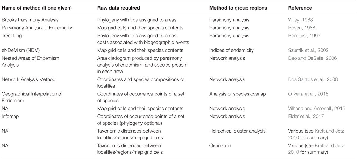
TABLE 1. Examples of quantitative methods for identifying areas of endemicity.

Defining Bioregions in Palaeodiversity Studies

Bringing these principals into a palaeontological framework is certainly possible, but there are a number of issues not impacting neontological data that must be taken into consideration. First, the majority of palaeontological datasets do not represent such fine sampling that bioregions may be defined at the resolution of mapping grid cells as in many modern neontological studies (Kreft and Jetz, 2010; Vilhena and Antonelli, 2015; Elder et al., 2017). Palaeontological datasets usually represent a “point cloud,” and it is individual localities which must be grouped together rather than adjacent grid cells. This precludes using methods such as constrained cluster analyses (e.g., Grimm, 1987) to ensure grid cells are only united with those adjacent to them. The solution is to use two hierarchical cluster analyses. The first one should group the localities or formations into clusters based on the palaeocoordinates in the manner of Button et al. (2017), thus ensuring that the bioregions defined form continuous, non-overlapping geographic areas. To ensure the areas being defined are areas of endemicity, the second cluster analysis should use taxonomic distances between the localities instead of geographic distances. A wide variety of taxonomic distance metrics exist (for summary see Koleff et al., 2003), but most work on same principle: comparing the number of taxa shared between pairs of localities to the numbers of taxa endemic to each.

The two cluster dendrograms are used to define the bioregions (see an example using the early Kungurian in Figures 1A,B; species occurrences and palaeocoordinates in Supplementary Data Sheet 1). We begin with each locality/formation representing a separate bioregion. Then, starting from the geographic dendrogram “tips,” one should work one’s way down the dendrogram toward the root, comparing each geographic cluster one by one to those in the taxonomic cluster dendrogram. If the localities grouped in the geographic clusters are also found to be grouped in a taxonomic cluster, then they represent a geographically continuous area of endemicity and may be grouped as a bioregion. A function has been written in R (Supplementary Data Sheet 1) to automate the comparison of geographic and taxonomic clusters, and also noting the geographic cluster node height of each defined bioregion (this will be of relevance below).

FIGURE 1

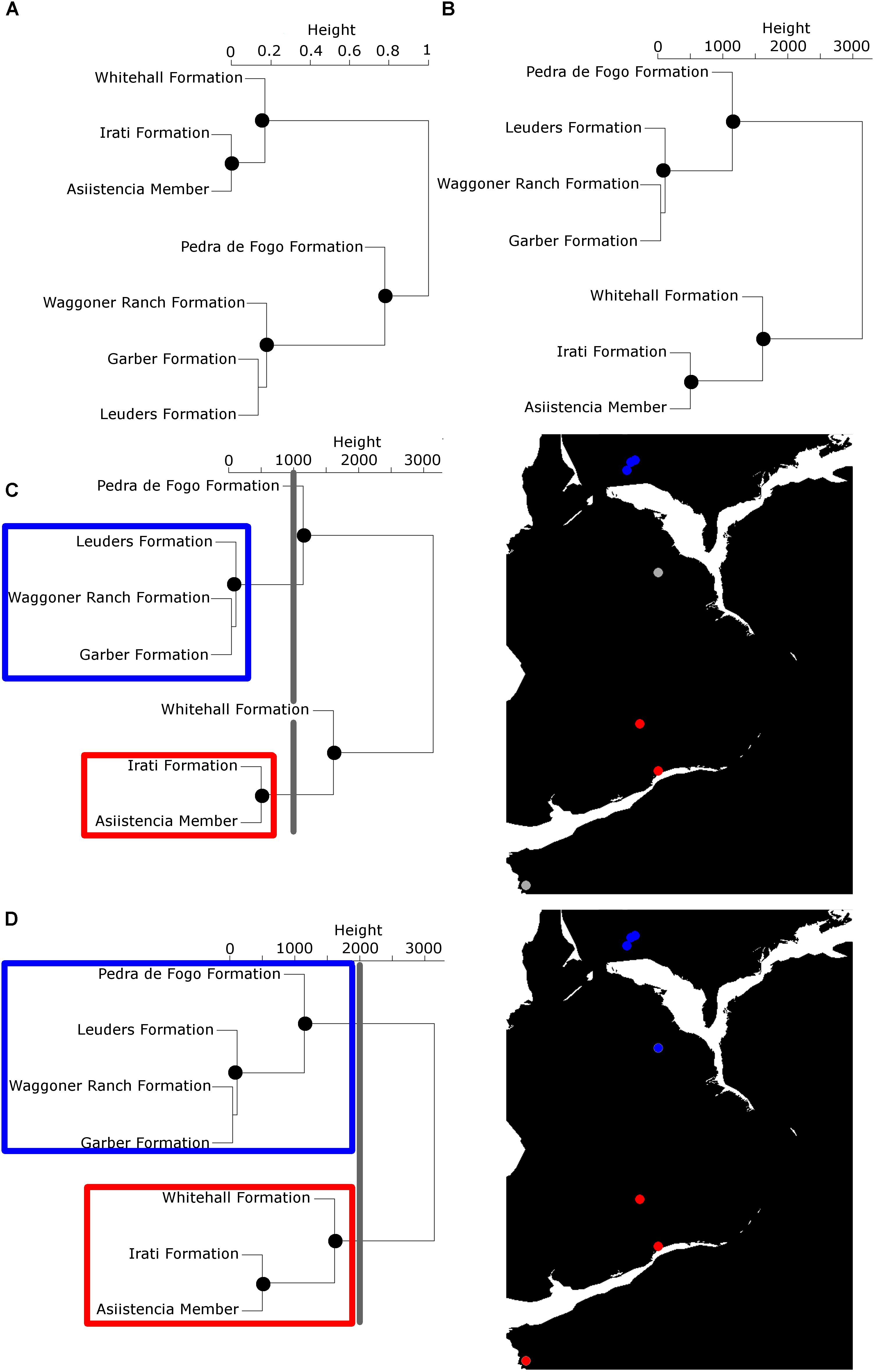
FIGURE 1. An illustration of the method used to define bioregions, using the early Kungurian tetrapod record as an example time bin. (A) UPGMA (“average”) Cluster dendrogram of formations based on taxonomic (Forbes^∗) distances (Alroy, 2015); (B) Cluster dendrogram of formations based on Euclidean geographic distances. Nodes illustrated with black dots in A and B are shared between the two and represent continuous geographic areas of endemicity (bioregions). (C,D) An illustration of how the spatial scale at which the bioregions are defined is controlled. (C) A geographic cluster node height of 1000 km is used, so all formations within 1000 km of each other are united in their bioregions. Four bioregions are defined: those in blue (palaeoequatorial North America), those in red (palaeotemperature South America), and two individual formations colored in gray on the map. (D) A geographic cluster node height of 2000 km is used. Two bioregions are defined: Those in blue (palaeoequatorial formations) and those in red (Southern palaeotemperature formations). Maps from the R package paleomap.

The second issue specific to palaeontological data is that the bioregions will change through time, as new barriers to dispersal develop and old barriers break down. It is therefore necessary that the procedure described above be applied to each time bin under study. This raises another consideration. Since the bioregions vary through time, when creating a curve of beta diversity (taxonomic differentiation between the bioregions) or regional diversity (species richness within the bioregions), one cannot standardize the bioregions themselves. One should instead ensure that the spatial scale of the diversity analyses is consistent in each time bin, by standardizing the geographic cluster node height at which the bioregions are grouped (Figures 1C,D). For example, if one chooses a geographic node height of 200, that means that all localities within 200 km of each other will be grouped into their bioregions (any localities that do not form taxonomic clusters with localities within that distance will be treated as their own bioregion). Multiple diversity curves should be created, each defining the bioregions at a different node height, to ensure that macroevolutionary patterns are examined at a range of spatial scales.

The final issue one must consider when applying this method to a palaeontological dataset is sampling heterogeneity. This issue is not absent from neontological datasets but is considerably more prevalent in the fossil record. Many of the issues surrounding the study of diversity in the fossil record have been discussed in the literature, and methods more robust to their influence have been suggested. When calculating both regional diversity within the bioregions, as well as taxonomic distance between bioregions (beta diversity), one must account for the fact that the bioregions have been sampled heterogeneously, preferably standardizing the sample size by coverage (Alroy, 2010; Chao and Jost, 2012; Close et al., 2018). Beta diversity estimates may be further biased by variations in the evenness of the relative abundance distribution when faunas are incompletely sampled (Beck et al., 2013; Brocklehurst et al., 2018b): with more uneven abundance distributions, where one or a few taxa are considerably more common than others, it is more likely that these taxa will be sampled in multiple bioregions and the beta diversity estimate will be lowered; on the other hand if the abundance distribution is more even it is more likely that different taxa will be sampled in different bioregions and the beta diversity estimates will be artificially raised. Brocklehurst et al. (2018b) suggested a method to correct for this issue by generating a null beta diversity expectation assuming a homogenous fauna sampled to the same extent as the observed fauna (the RAC beta diversity estimate).

Another issue specific to beta diversity study in the fossil record, particularly in a global context, is heterogeneous geographic spread of the sampling. While the geographic spread of sampling is quantifiable [Close et al. (2017) summarized the various metrics, ultimately favoring minimum spanning tree length], thus far no solution has been proposed to the impact this may have on beta diversity estimates. If one starts with a null expectation that greater geographic distance between bioregions will lead to greater taxonomic distance, then increasing the geographic spread of sampling will be expected to artificially increase the beta diversity estimate by adding larger taxonomic distances. Here it is proposed to mitigate this issue by restricting the taxonomic distances included in the calculation of beta diversity, removing the pairwise comparisons between bioregions separated by geographic distances outside an upper and lower bound (Figure 2). These bounds may be defined as the maximum and minimum geographic distance between bioregions observed in the time bin with the most restricted geographic spread of sampling (Figure 2A). Hereafter, this method will be described as geographic-spread-subsampling (GSS).

FIGURE 2

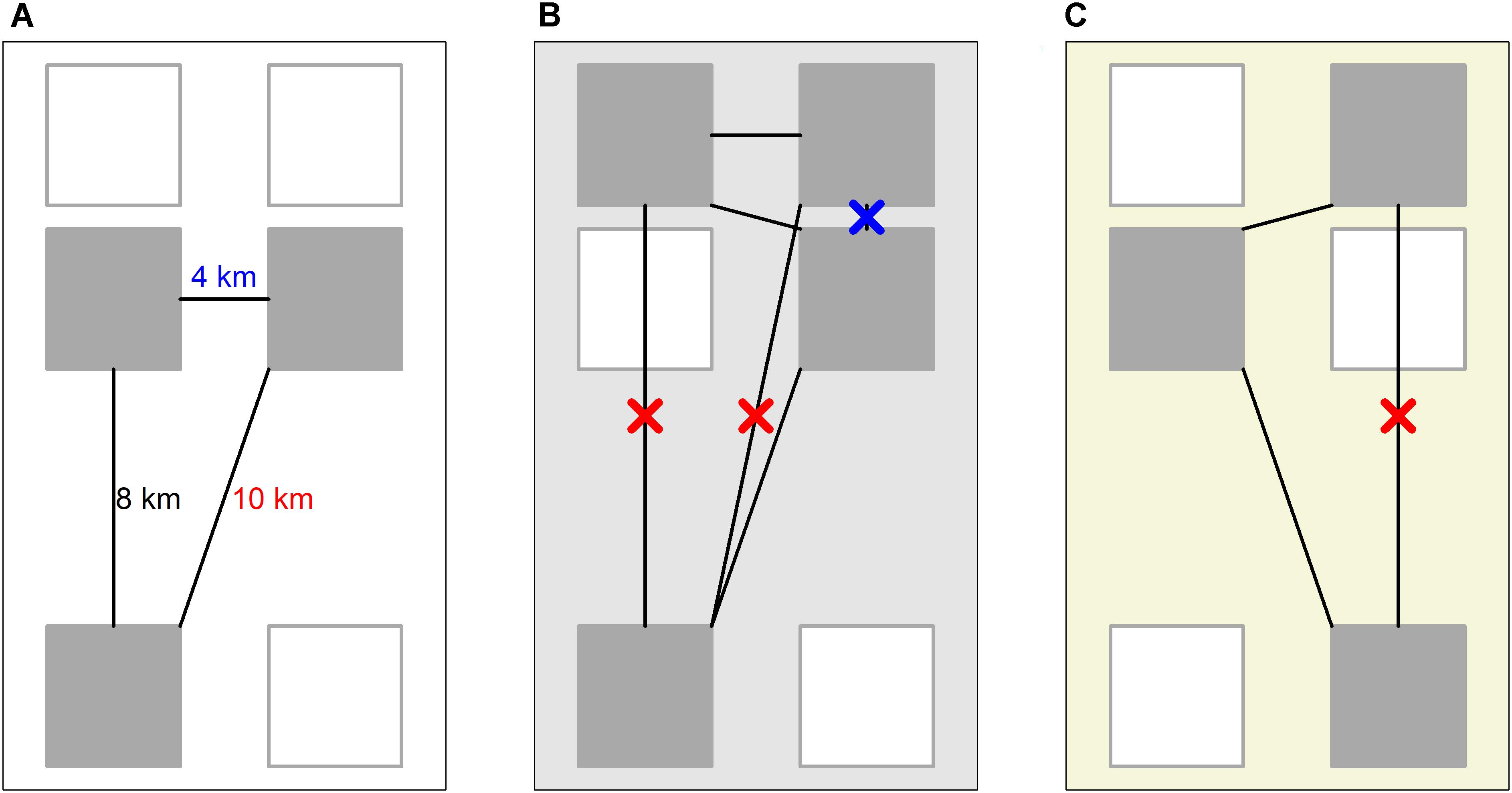
FIGURE 2. An illustration of Geographic Spread Subsampling. Each large colored rectangle (white, light gray, and yellow) represents the fossil record of a particular time bin. There are six localities available for sampling (gray rectangles), those unsampled filled white instead of gray. Time bin A is the bin with the lowest geographic spread of sampling. The largest (red) and smallest (blue) geographic distances between the localities define which pairs of localities will be included in beta diversity estimates of subsequent time bins. In B and C, those pairs of localities separated by greater (red crosses) or smaller (blue cross) geographic distances than the bounds defined by time bin A are not considered.

Workflow: Beta Diversity of Palaeozoic Tetrapods

The workflow described above was applied to an analysis of beta diversity of Carboniferous and Permian tetrapods. A dataset of tetrapod specimens present in each formation was compiled from a variety of sources, including the published literature, observations from museum specimens and the Paleobiology Database accessed from the fossilworks website¹. Formations were used as the minimum spatial scale in order to minimize the number of singletons; for better sampled records, one might be able to examine groupings at finer spatial scales, like localities, to compare individual habitats. Formations containing a single taxon were discarded. An attempt was made to incorporate specimens not yet assigned to species level. If there were named species of the higher taxon thought to be represented by the indeterminate specimen, the indeterminate specimen was assigned to the most abundant named species of that higher taxon in the same formation. If there were no other species assigned to that higher taxon in that formation, then the specimen would be assigned to the most abundant species of that higher taxon in the geographically nearest contemporary formation. If there are no named species of that higher taxon in that time bin, then the specimen will be assigned to “indeterminate [taxon].” These datasets are present in the Supplementary Data Sheet 1.

For each time bin (informal substages created by dividing the international stages in half), the pairwise taxonomic distances between each formation were calculated using the modified Forbes index (Alroy, 2015), applying the RAC correction (Brocklehurst et al., 2018b). This was done in R version 3.3.2 (R Core Team, 2016), using the functions provided by Brocklehurst et al. (2018b). The pairwise distance matrix was subjected to a hierarchical cluster analysis using the hclust function from the R package vegan (Oksanen et al., 2017), using UPGMA clustering following the recommendations of Kreft and Jetz (2010). The same function was used to perform the cluster analysis using Euclidean geographic distances.

The two cluster dendrograms were used to group the formations into bioregions using the procedure described above. The bioregions in each time bin were defined at three spatial scales: using geographic cluster node heights of 0 (each formation representing its own bioregion), 200 and 2000 km. This incorporated a range of spatial scales, from local to continental. Beta diversity was calculated as the mean pairwise taxonomic distance between the bioregions. Subsampling was incorporated to a coverage of 0.4, following the recommended minimum of Alroy (2010).

Two assessments of beta diversity were carried out at each node height, one incorporating geographic spread subsampling (GSS) and one not. For the assessment using GSS, after bioregions had been defined at each spatial scale, the minimum spanning tree connecting all bioregions was identified using the function spantree, also from the package vegan. The total length of the minimum spanning tree of each time bin was used to identify which bin had the smallest geographic spread of sampling (Figure 3). The maximum and minimum distances between bioregions in that time bin were used to identify which bioregion pairs would be included in the calculation of beta diversity. The upper and lower distance bounds used at each spatial scale are given in Table 2.

FIGURE 3

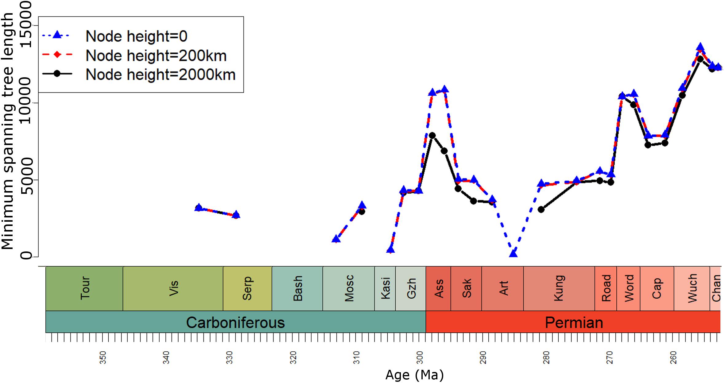
FIGURE 3. Geographic spread of sampling of tetrapods in each time bin, measured as the minimum spanning tree length between bioregions defined at three geographic cluster node heights.

TABLE 2

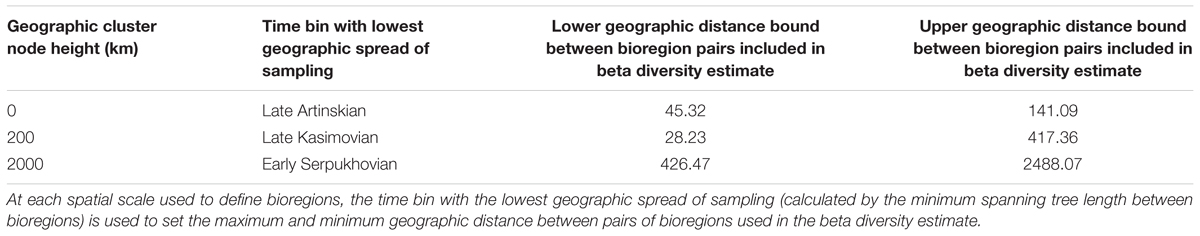
TABLE 2. Details of the time bins used to define the parameters of Geographic Spread Subsampling.

Results

Using the proposed workflow, very few time bins could be assessed for beta diversity during the first half of the Carboniferous. This is due to the necessity for at least three formations in each time bin to perform a cluster analysis. However, the data is of sufficient quality to provide results for most time bins from the Moscovian onward.

The raw RAC beta diversity estimates (correction by GSS not applied) produce similar results at different spatial scales during the Carboniferous (Figure 4A); not only are the curves showing similar trends, but the absolute values obtained are very similar. All three beta diversity estimates remain above 0.9 during the latest Carboniferous stages. However, during the Cisuralian (early Permian), there is a divergence between the curves. When bioregions are defined at cluster node heights of 0 and 200 km, the beta diversity estimates fall noticeably during the Asselian, Sakmarian and early Artinskian. However, at node heights of 2000 km, the estimates remain high. The late Artinskian does not allow bioregions to be defined at node heights of 200 or 2000 km as the greatest distance between formations is 141 km. Nevertheless, the early Kungurian results at these spatial scales are similar to those in the Asselian and Sakmarian.

FIGURE 4

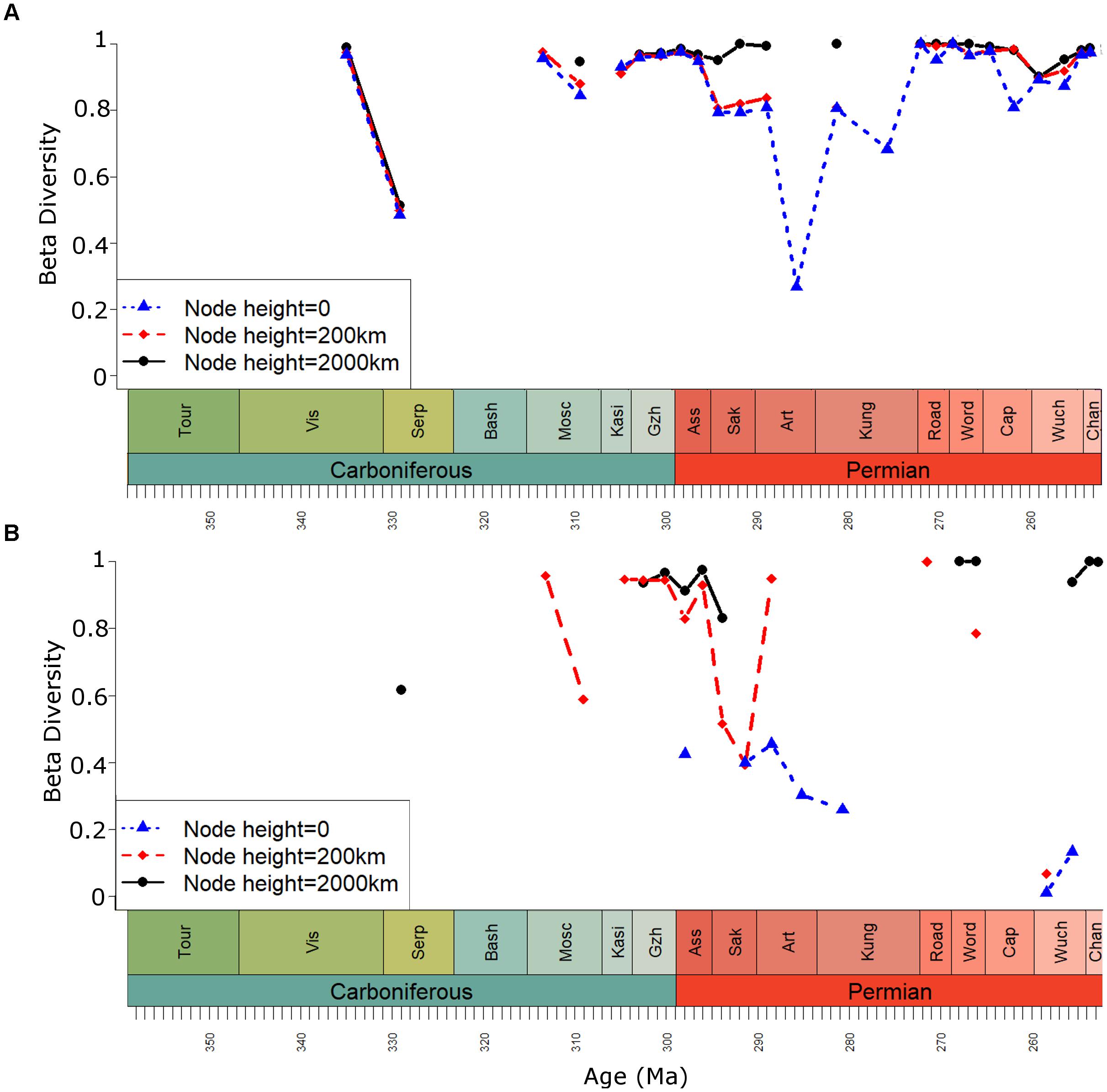
FIGURE 4. Beta diversity of Palaeozoic tetrapods (mean pairwise taxonomic distance between each bioregion). Bioregions defined at three geographic cluster node heights. (A) No geographic spread subsampling; (B) With geographic spread subsampling.

In the Guadalupian (middle Permian), beta diversity curves with bioregions defined at node heights 0 and 200 km rise to produce similar values to when the bioregions are defined at 2000 km. These values remain close to 1 for the rest of the Permian.

The curves produced by the analyses incorporating the GSS method (Figure 4B) to correct for variation in the geographic spread in sampling illustrate a potential pitfall of this method: in cases where the geographic sampling is particularly patchy, many time bins will have to be removed if none of their localities are separated by geographic distances between the upper and lower bounds used for that time series. The Palaeozoic tetrapod record has long been known to have a poor geographic spread in geographic sampling (Kemp, 2006; Benson et al., 2013; Brocklehurst et al., 2013, 2017), and beta diversity estimates calculated at all spatial scales contain substantial gaps. This is particularly problematic when bioregions are defined at a node height of 0 (when each formation represents a separate bioregion). At this node height, the upper and lower distance bounds used in the GSS method are defined by the late Artinskian: the minimum distance is 45 km and the maximum is only 141. This extremely narrow range greatly limits the number of time bins that can be included; no beta diversity estimates are available at this node height from the entire Carboniferous or the Guadalupian (middle Permian).

Nevertheless, the GSS curves calculated when bioregions are defined at node heights of 200 and 2000 km do cover the Carboniferous and Permian boundary, providing information on changes in faunal provinciality at this crucial time at both local and global spatial scales. The two beta diversity curves are both high during the latest Carboniferous. However, in the earliest Permian the two signals begin to diverge. When beta diversity is calculated at more local scales, a substantial decrease is noted during the Asselian and in particular the Sakmarian. However, when bioregions are defined on continental scales (node height of 2000 km) beta diversity remains high.

Discussion

The issue of spatial scale in the study of alpha and beta diversity has been extensively discussed in the ecological literature (Palmer and White, 1994; Rosenweig, 1995; Whittaker et al., 2001; Field et al., 2009; Keil et al., 2012; Barton et al., 2013). Its importance lies not only in the fact that different organisms have different dispersal capacity, but also in the fact that different factors, both environmental and organismal, will control the diversity observed within a particular scale of bioregion (for summary see Barton et al., 2013). Hypothetically, if one started at a particular locality and then slowly increased the sampling area, one would first expect to see a rapid increase in the number of species included in the sample, as new habitats will frequently be added to the dataset. Eventually, the rate of addition of new environments and niches will slow, as will the addition of new species to the pool. Once the sampling area begins to include areas covering multiple continents, isolation by large-scale physical barriers to dispersal, such as mountain ranges and oceans, combined with regional extinction and taxon replacement will again cause the number of species in the pool to increase rapidly with increased sampling area.

In historical diversity and biogeography studies using palaeontological data, the issue of spatial scale is even more critical. Not only will diversity estimates (whether alpha or beta) vary depending on the spatial scale at which the bioregion is defined, but patterns and trends through time will also vary. The dispersal ability of the organisms under study will change through time both due to phenotypic evolution changing locomotion methods and environmental tolerance, and due to geological and environmental changes. The degree of environmental heterogeneity will vary through time as well, meaning that environmental barriers will have varying importance relative to physical barriers e.g., in periods such as the late Cretaceous where latitudinal temperature gradients were reduced relative to today (Huber et al., 1995; Upchurch G. R. et al., 2015; Lunt et al., 2016), dispersal along latitudinal gradients might in theory have been easier and areas of endemicity might be expected to be larger. This is particularly the case for ectothermic vertebrates, whose ranges are heavily constrained by their thermal tolerances, but which during the late Cretaceous were able to occupy wider latitudinal ranges (Markwick, 1998; Amiot et al., 2004). As such, it is important that paleontologists study not only trends in alpha and beta diversity through time, but also study variation in the trends observed at different spatial scales, as this can provide vital information about the dispersal abilities of the organisms and the importance of regional- and continental-scale barriers. Analysis of biogeography where geography is treated as a continuous variable will miss such signals, as the only spatial grain size considered is the smallest possible.

The information that may be obtained from examining beta diversity at different spatial scales (with rigorously defined bioregions) is apparent in the Palaeozoic tetrapod dataset. Similar beta diversity values are obtained at very different spatial scales during the late Carboniferous. The fact that the taxonomic distances between individual formations, which are in some cases geographically very close, are almost identical to the taxonomic distances between bioregions uniting formations up to 2000 km apart, indicates that the principal barriers to tetrapod dispersal were operating at local scales, and presumably represent local environmental heterogeneity. However, during the Cisuralian, there is a divergence between the curves. When bioregions are defined at cluster node heights of 0 and 200 km, the beta diversity estimates fall noticeably during the Asselian and Sakmarian. However, at node heights of 2000 km, the estimates remain high. This divergence indicates a shift in the nature of tetrapod dispersal, with a reduced importance of the more local barriers (leading to the decrease in beta diversity when bioregions are defined at a node height of 200 km) and in increased importance of the large-scale physical/geographical barriers between continents.

These patterns may also be seen by examining the taxonomic cluster dendrograms. During the late Carboniferous there is no distinct separation between the European and North American formations; they do not form discrete clusters. While this is still the case during the Asselian (Figure 4), one interesting grouping is identified in both the geographic and taxonomic cluster dendrograms: a grouping of the formations from western North America (New Mexico, Colorado, Utah and Arizona). These formations are separated from the eastern formations by a shallow inland seaway known as the Hueco seaway (Lucas et al., 2011). This cluster is observed from the Asselian for as long as a record is available from this region (Figure 4). The early Sakmarian represents the first time that the European formations form discrete clusters separate from those of North America, a separation that again continues for as long as a European record is preserved (Figure 5). Again, this may be attributed to physical barriers between the continents: the Variscan orogeny experienced a period of increased uplift toward the end of the Carboniferous that continued through the Cisuralian (Badham, 1982; Dewey, 1982; Rowley et al., 1985; Cleal et al., 2009). The European formations mostly represent intermontane basins within the orogeny (Cleal et al., 2009), and the increased uplift has been suggested to have greatly limited dispersal between these basins and the North American formations during the early Permian. The North American formations do not from a discrete taxonomic cluster solely due to the Speiser Shale, which contains no species overlapping with contemporary formations. The large taxonomic distances between this formation and those geographically close does not appear to be a result of sampling; coverage has been standardized and formations not reaching the requisite levels of coverage would have been dropped. This might be due to taxonomic over-splitting, a problem noted as affected studies of Carboniferous and Permian tetrapods (Brocklehurst and Fröbisch, 2014); genera present in this formation, such as Brachydectes and Acroplous, are present elsewhere. This perhaps indicates that further exploration into methods incorporating phylogeny into the definition of bioregions is warranted.

FIGURE 5

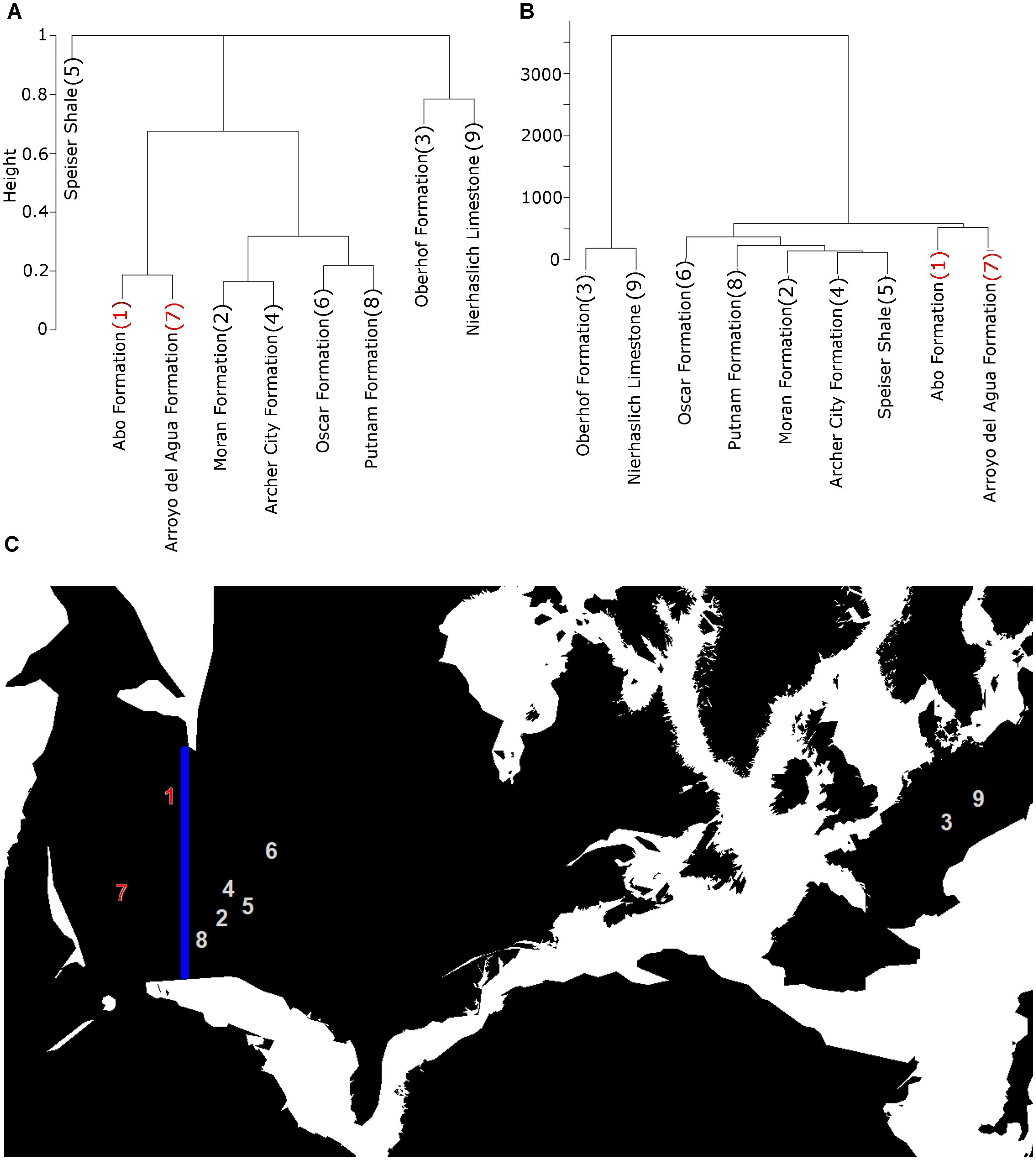
FIGURE 5. Illustration of the early Sakmarian formations, showing the taxonomic and geographic clustering of the European formations and those in North America west of the Hueco Seaway (seaway not visible on this map). (A) Cluster dendrogram based of taxonomic distances; (B) Cluster dendrogram based on geographic distances; (C) Location of the formations. The blue line represents the division between those west and east of the Hueco Seaway. Numbers on cluster dendrogram labels correspond to labels on the map. Maps from the R package paleomap.

The contradictions between the beta diversity estimates provide an explanation of the discrepancy between the results of Dunne et al. (2018) and Brocklehurst et al. (2018a). The former study, using k-means clustering based on geographic coordinates, grouped localities into smaller areas than the latter, which divided the earth into regions bounded by mountain ranges, inland seaways and latitudinal barriers, with the bioregions mostly being on the scale of continents. The Dunne et al. (2018). study identified the reduced provinciality caused by the breakdown of the more local environmental barriers, while the Brocklehurst et al. (2018a) study identified the increased importance of continental scale barriers, causing reduced dispersal between the bioregions used. Both these studies, and the results obtained here, reject the earlier work of Sahney et al. (2010), who suggested that faunal provinciality at this time was controlled by the rainforest collapse. The idea put forward was that the equatorial rainforests prevalent during the Carboniferous declined during the latest Carboniferous, leaving small islands of forest separated by more open environments, which represented barriers to dispersal and lead to increased beta diversity in the early Permian. This theory is not borne out by the data presented here. The more local environmental barriers are found to break down during the early Permian, and the principal barriers to tetrapod dispersal are found to operate on a more continental scale.

Interestingly, while an “island biogeography” effect, posited by Sahney et al. (2010) is not observed at the end of the Carboniferous, it is toward the end of the Cisuralian. The beta diversity estimates when bioregions are defined at local scales, (node heights of 0 and 200), which had been low throughout much of the Cisuralian, rise rapidly during the Kungruian and Roadian, reaching similar values to those obtained at node heights of 2000 km (Figure 4A). This shift coincides with a substantial turnover of tetrapods, with a fauna characterized by a diverse array of amphibians, pelycosaurian-grade synapsids, particularly carnivorous sphenacodontids and herbivorous edaphosaurids, and captorhinids, transitioning to one dominated by therapsid synapsids, with diversity of parareptiles increased and amphibian diversity substantially reduced (Olson, 1962, 1966; Kemp, 2006; Sahney and Benton, 2008; Ruta et al., 2011; Benton, 2012; Benson and Upchurch, 2013; Brocklehurst et al., 2013, 2017; Brocklehurst, 2018). A mass extinction is also thought to have occurred at this time (Olson, 1982; Sahney and Benton, 2008; Brocklehurst et al., 2017; Brocklehurst, 2018). The sediments of the latest Kungurian Clear Fork Group record an environmental shift toward seasonal dryness and ever-increasing aridity, with a reduction in the number of perennial water sources (Olson, 1958). The uppermost deposits formed almost entirely from anhydrites (Olson, 1958). During this aridification episode, tetrapods became more restricted in their distribution, with their fossils concentrating around the few permanent water sources rather than the intervening sediments. This may explain how the two Roadian formations of North American, the San Angelo (Texas) and Chickasha (Oklahoma), despite being close geographically and having a similar set of higher-level taxa present, in fact show no overlap at the species level (Olson, 1965; Brocklehurst et al., 2017).

Conclusion

As the use of “Big Data” in paleontology becomes more common, the importance of automation is increasing. However, certain analytical decisions have required more participation from the researcher, making such analyses more time consuming to apply to global datasets over large timescales. The procedure discussed here for defining bioregions in palaeontological datasets provides automation for a process that would previously have either required the increased input from the researcher, or the use of such arbitrary methods as using the continents as bioregions or treating geography as a continuous character. The data needed for defining the bioregions (taxonomic occurrences/abundances and palaeo-coordinates) are included in widely used sources such as the Paleobiology Database. The Geographic Spread Subsampling method, while perhaps not well suited to the overly patchily sampled Paleozoic tetrapod record studied here, would be better applied to “big data” analyses, and is also easily automated. It is important to remember that increased automation in paleontology does not have to be at the expense of rigor and biological realism.

Author Contributions

NB and JF conceived the project. NB developed the dataset, designed the method, and analyzed the data. NB wrote the manuscript with contributions from JF.

Funding

This study was financially supported by Deutsche Forschungsg-emeinschaft grant no. FR 2457/5-1 awarded to JF. The publication of this article was funded by the Open Access Fund of the Leibniz Association and the Museum für Naturkunde Berlin.

Conflict of Interest Statement

The authors declare that the research was conducted in the absence of any commercial or financial relationships that could be construed as a potential conflict of interest.

Acknowledgments

We would like to thank Roger Benson, Roger Close, Richard Butler, and Emma Dunne for helpful comments and discussion.

Supplementary Material

The Supplementary Material for this article can be found online at: https://www.frontiersin.org/articles/10.3389/feart.2018.00200/full#supplementary-material

DATA SHEET S1 | The custom R code used to group localities into bioregions, and the numbers of tetrapod specimens in each formation in each time bin.

Footnotes

1. ^http://fossilworks.org/

References

Allwood, J., Gleeson, D., Mayer, G., Daniels, S., Beggs, J. R., and Buckley, T. R. (2010). Support for vicariant origins of the New Zealand Onychophora. J. Biogeogr. 37, 669–681. doi: 10.1111/j.1365-2699.2009.02233.x

CrossRef Full Text | Google Scholar

Alroy, J. (2010). Geographical, environmental and intrinsic biotic controls on Phanerozoic marine diversification. Palaeontology 53, 1211–1235. doi: 10.1111/j.1475-4983.2010.01011.x

CrossRef Full Text | Google Scholar

Alroy, J. (2015). A new twist on a very old binary similarity coefficient. Ecology 96, 575–586. doi: 10.1890/14-0471.1

PubMed Abstract | CrossRef Full Text | Google Scholar

Amiot, R., Lécuyer, C., Buffetaut, E., Fluteau, F., Legendre, S., and Martineau, S. (2004). Latitudinal temperature gradient during the Cretaceous Upper Campanian- Middle Maastrichtian: δ18O record of continental vertebrates. Earth Planet. Sci. Lett. 226, 255–272. doi: 10.1016/j.epsl.2004.07.015

CrossRef Full Text | Google Scholar

Andow, D. A., Kareva, P. M., Levin, S. A., and Okubo, A. (1990). Spread of invading organisms. Landsc. Ecol. 4, 177–188. doi: 10.1007/BF00132860

CrossRef Full Text | Google Scholar

Badham, J. P. N. (1982). Strike-slip orogens—an explanation for the Hercynides. J. Geol. Soc. 139, 493–504. doi: 10.1144/gsjgs.139.4.0493

CrossRef Full Text | Google Scholar

Barton, P. S., Cunningham, S. A., Manning, A. D., Gibb, H., Lindenmayer, D. B., and Didham, R. K. (2013). The spatial scaling of beta diversity. Glob. Ecol. Biogeogr. 22, 639–647. doi: 10.1111/geb.12031

CrossRef Full Text | Google Scholar

Beck, J., Holloway, J. D., and Schwanghart, W. (2013). Undersampling and the measurement of beta diversity. Methods Ecol. Evol. 4, 370–382. doi: 10.1111/2041-210x.12023

CrossRef Full Text | Google Scholar

Benson, R. B., Butler, R. J., Alroy, J., Mannion, P. D., Carrano, M. T., and Lloyd, G. T. (2016). Near-stasis in the long-term diversification of Mesozoic tetrapods. PLoS Biol. 14:e1002359. doi: 10.1371/journal.pbio.1002359

PubMed Abstract | CrossRef Full Text | Google Scholar

Benson, R. B. J., Mannion, P. D., Butler, R. J., Upchurch, P., Goswami, A., and Evans, S. E. (2013). Cretaceous tetrapod fossil record sampling and faunal turnover: implications for biogeography and the rise of modern clades. Palaeogeogr. Palaeoclim. Paleoecol. 372, 88–107. doi: 10.1016/j.palaeo.2012.10.028

CrossRef Full Text | Google Scholar

Benson, R. B. J., and Upchurch, P. (2013). Diversity trends in the establishment of terrestrial vertebrate ecosystems: interactions between spatial and temporal sampling biases. Geology 41, 43–46. doi: 10.1130/G33543.1

Google Scholar

Benton, M. J. (2012). No gap in the Middle Permian record of terrestrial vertebrates. Geology 40, 339–342. doi: 10.1098/rspb.2011.0439

PubMed Abstract | CrossRef Full Text | Google Scholar

Brocklehurst, N. (2018). An examination of the impact of Olson’s extinction on tetrapods from Texas. PeerJ 6:e4767. doi: 10.7717/peerj.4767

PubMed Abstract | CrossRef Full Text | Google Scholar

Brocklehurst, N., Day, M. O., and Fröbisch, J. (2018a). Accounting for differences in species frequency distributions when calculating beta diversity in the fossil record. Methods Ecol. Evol. 9, 1409–1420. doi: 10.1111/2041-210X.13007

CrossRef Full Text | Google Scholar

Brocklehurst, N., Dunne, E. M., Cashmore, D. D., and Fröbisch, J. (2018b). Physical and environmental drivers of Palaeozoic tetrapod dispersal across Pangaea. Nat. Commun. (in press).

Brocklehurst, N., Day, M. O., Rubidge, B. R., and Fröbisch, J. (2017). Olson’s Extinction and the latitudinal biodiversity gradient of tetrapods in the Permian. Proc. R. Soc. B 284:20170231. doi: 10.1098/rspb.2017.0231

PubMed Abstract | CrossRef Full Text | Google Scholar

Brocklehurst, N., and Fröbisch, J. (2014). Current and historical perspectives on the completeness of the fossil record of pelycosaurian-grade synapsids. Palaeogeog. Palaeoclim. Palaeoecol. 399, 114–126. doi: 10.1016/j.palaeo.2014.02.006

CrossRef Full Text | Google Scholar

Brocklehurst, N., Kammerer, C. F., and Fröbisch, J. (2013). The early evolution of synapsids, and the influence of sampling on their fossil record. Paleobiology 39, 470–490. doi: 10.1666/12049

CrossRef Full Text | Google Scholar

Brooks, D. R. (1990). Parsimony analysis in historical biogeography and coevolution: methodological and theoretical update. Syst. Zool. 39, 14–30. doi: 10.2307/2992205

CrossRef Full Text | Google Scholar

Brooks, D. R., Van Veller, M. G. P., and McLennan, D. (2001). How to do BPA, really. J. Biogeogr. 28, 345–358. doi: 10.1046/j.1365-2699.2001.00545.x

CrossRef Full Text | Google Scholar

Brouckaert, R., Lemy, P., Dunn, M., Greenhill, S. J., Alekseyenko, A. V., Drummond, A. J., et al. (2012). Mapping the origins and expansion of the Indo-European language family. Science 377, 957–960. doi: 10.1126/science.1219669

PubMed Abstract

Button, D. J., Lloyd, G. T., Ezcurra, M. D., and Butler, R. J. (2017). Mass extinctions drove increased global faunal cosmopolitanism on the supercontinent Pangaea. Nat. Commun. 8:733. doi: 10.1038/s41467-017-00827-7

PubMed Abstract | CrossRef Full Text | Google Scholar

Chao, A., and Jost, L. (2012). Coverage-based rarefaction and extrapolation: standardising samples by completeness rather than size. Ecology 93, 2533–2547. doi: 10.1890/11-1952.1

CrossRef Full Text | Google Scholar

Cleal, C. J., Opluštil, B. A., Tenchov, T. Y., Abbink, O. A., Bek, K., Bimitrova, T., et al. (2009). Late Moscovian terrestrial biotas and palaeoenvironments of Variscan Euramerica. Neth. J. Geosci. 88, 181–278. doi: 10.1017/S0016774600000846

CrossRef Full Text | Google Scholar

Close, R. A., Benson, R. B. J., Upchurch, P., and Butler, R. J. (2017). Controlling for the species-area effect supports constrained long-term Mesozoic terrestrial vertebrate diversification. Nat. Commun. 8:15381. doi: 10.1038/ncomms15381

PubMed Abstract | CrossRef Full Text | Google Scholar

Close, R. A., Evers, S. W., Alroy, J., and Butler, R. J. (2018). How should we estimate diversity in the fossil record? Testing richness estimators using sampling standardised discovery curves. Methods Ecol. Evol. 9, 1386–1400. doi: 10.1111/2041-210X.12987

CrossRef Full Text | Google Scholar

Deo, A. J., and DeSalle, R. (2006). Nested areas of endemism analysis. J. Biogeogr. 33, 1511–1526. doi: 10.1111/j.1365-2699.2006.01559.x

CrossRef Full Text | Google Scholar

Dewey, J. F. (1982). Plate tectonics and the evolution of the British Isles. J. Geol. Soc. 139, 371–412. doi: 10.1073/pnas.0805607106

PubMed Abstract | CrossRef Full Text | Google Scholar

Dinerstein, E., Olson, D. M., Graham, D. J., Webster, A. L., Primm, S. A., Bookbinder, M. P., et al. (1995). A Conservation Assessment of the Terrestrial Ecoregions of Latin America and the Caribbean. Washington, DC: World Wildlife Fund and World Bank.

Google Scholar

Dos Santos, D. A., Fernández, H. R., Cuezzo, M. G., and Domínguez, E. (2008). Sympatry inference and network analysis in biogeography. Syst. Biol. 57, 432–448. doi: 10.1080/10635150802172192

Google Scholar

Dunhill, A. M., Bestwick, J., Narey, H., and Sciberras, J. (2016). Dinosaur biogeographical structure and Mesozoic continental fragmentation: a network-based approach. J. Biogeogr. 4, 1691–1704. doi: 10.1111/jbi.12766

CrossRef Full Text | Google Scholar

Dunne, E. M., Close, R. A., Button, D. J., Brocklehurst, N., Cashmore, D. D., Lloyd, G. T., et al. (2018). Diversity change during the rise of tetrapods and the impact of the ‘Carboniferous rainforest collapse’. Proc. R. Soc. B 285:20172730. doi: 10.1098/rspb.2017.2730

PubMed Abstract | CrossRef Full Text | Google Scholar

Elder, D., Guedes, T., Zizka, A., Rosvall, M., and Antonelli, A. (2017). Infomap Bioregions: interactive mapping of biogeographical regions from species distributions. Syst. Biol. 66, 197–204. doi: 10.1093/sysbio/syw087

PubMed Abstract | CrossRef Full Text | Google Scholar

Eldridge, N., and Gould, S. J. (1972). “Punctuated equilibrium, an alternative to phyletic gradualism,” in Models in Palaeobiology, ed. T. J. M. Schopf (San Francisco, CA: Freedman Cooper), 540–547.

Ferrari, A. (2017). Biogeographical units matter. Aust. Syst. Bot. 30, 391–402. doi: 10.1071/SB16054

CrossRef Full Text | Google Scholar

Field, R., Hawkins, B. A., Cornell, H. V., Currie, D. J., Diniz-Filho, J. A. F., Guégan, J. F., et al. (2009). Spatial species-richness gradients across scales: a meta-analysis. J. Biogeogr. 36, 132–147. doi: 10.1111/ele.12277

PubMed Abstract | CrossRef Full Text | Google Scholar

Grimm, E. C. (1987). CONISS: a FORTRAN 77 program for stratigraphically constrained cluster analysis by the method of incremental sum of squares. Comput. Geosci. 13, 13–35. doi: 10.1016/0098-3004(87)90022-7

CrossRef Full Text | Google Scholar

Hausdorf, B. (2002). Units in biogeography. Syst. Biol. 51, 648–652. doi: 10.1080/10635150290102320

PubMed Abstract | CrossRef Full Text | Google Scholar

Huber, B. T., Hodell, D. A., and Hamilton, C. P. (1995). Middle-Late Cretaceous climate of the southern high latitudes: stable isotopic evidence for minimal equator-to-pole thermal gradients. Geol. Soc. Am. Bull. 107, 1164–1191. doi: 10.1130/0016-7606(1995)107<1164:MLCCOT>2.3.CO;2

CrossRef Full Text

Kaiser, G. W., Lefkovitch, L. P., and Howden, H. F. (1972). Faunal provinces in Canada as exemplified by mammals and birds: a mathematical consideration. Can. J. Zool. 50, 1087–1104. doi: 10.1139/z72-146

Google Scholar

Keil, P., Schweiger, O., Kühn, I., Kunin, W. E., Kuussaari, M., Settele, J., et al. (2012). Patterns of beta diversity in Europe: the role of climate, land cover and distance across scales. J. Biogeogr. 39, 1473–1486. doi: 10.1111/j.1365-2699.2012.02701.x

CrossRef Full Text | Google Scholar

Kemp, T. S. (2006). The origin and early radiation of the therapsid mammal-like reptiles: a palaeobiological hypothesis. J. Evol. Biol. 19, 1231–1247. doi: 10.1111/j.1420-9101.2005.01076.x

PubMed Abstract | CrossRef Full Text | Google Scholar

Kirkpatrick, M., and Barton, N. H. (1997). Evolution of a species’ range. Am. Nat. 150, 1–23. doi: 10.1086/286054

PubMed Abstract | CrossRef Full Text | Google Scholar

Koleff, P., Gaston, K. J., and Lennon, J. J. (2003). Measuring beta diversity for presence-absence data. J. Anim. Ecol. 72, 367–382. doi: 10.1046/j.1365-2656.2003.00710.x

CrossRef Full Text | Google Scholar

Kreft, H., and Jetz, W. (2010). A framework for delineating biogeographical regions based on species distributions. J. Biogeogr. 37, 2029–2053. doi: 10.1111/j.1365-2699.2010.02375.x

CrossRef Full Text | Google Scholar

Layou, K. M. (2007). A quantitative null model of additive diversity partitioning: examining the response of beta diversity to extinction. Paleobiology 33, 116–124. doi: 10.1666/06025.1

CrossRef Full Text | Google Scholar

Lemmon, A. R., and Lemmon, E. M. (2008). A likelihood framework for estimating phylogeographic history on a continuous landscape. Syst. Biol. 57, 544–561. doi: 10.1080/10635150802304761

PubMed Abstract | CrossRef Full Text | Google Scholar

Linder, H. P. (2001). On areas of endemism, with an example from the African Restionaceae. Syst. Biol. 50, 892–912. doi: 10.1080/106351501753462867

PubMed Abstract | CrossRef Full Text | Google Scholar

Lloyd, G. T., and Soul, L. (2015). Detecting phylogenetic signals of endemism and dispersal: the effects of Pangaean breakup and avian flight on Mesozoic Dinosaurs. J. Vert. Paleontol. Program Abstr. 2015, 165–166.

Lucas, S. G. (2011). Traces of a Permian Seacoast: Prehistoric Trackways National Monument. New Mexico: New Mexico Museum of Natural History and Science.

Google Scholar

Lunt, D. J., Farnsworth, A., Loptson, C., Foster, G. L., Markwick, P., O’Brien, C. L., et al. (2016). Palaeogeographic controls on climate and proxy interpretation. Clim. Past 12, 1181–1198. doi: 10.5194/cp-12-1181-2016

CrossRef Full Text | Google Scholar

Markwick, P. J. (1998). Fossil crocodilians as indicators of Late Cretaceous and Cenozoic climates; implications for using palaeontological data in reconstructing palaeoclimate. Palaeogeogr. Palaeoclimatol. Palaeoecol. 137, 205–271. doi: 10.1016/S0031-0182(97)00108-9

CrossRef Full Text | Google Scholar

Morrone, J. J. (1994). On the identification of areas of endemism. Syst. Biol. 43, 438–441. doi: 10.1093/sysbio/43.3.438

CrossRef Full Text | Google Scholar

Murray, A. M. (2001). The fossil record and biogeography of the Cichlidae (Actinopterygii: Labroidei). Biol. J. Linn. Soc. 74, 517–532. doi: 10.1111/j.1095-8312.2001.tb01409.x

CrossRef Full Text | Google Scholar

Nylander, S., Lemy, P., Bruyn, M. D., Suchard, M. A., Pfeil, B. E., Walsh, N., et al. (2014). On the biogeography of Centipeda: a species-tree diffusion approach. Syst. Biol. 63, 178–191. doi: 10.1093/sysbio/syt102

PubMed Abstract | CrossRef Full Text | Google Scholar

O’Donovan, C., Meade, A., and Venditti, C. (2018). Dinosaurs reveal the geographical signature of an evolutionary radiation. Nat. Ecol. Evol. 2, 452–458. doi: 10.1038/s41559-017-0454-6

PubMed Abstract | CrossRef Full Text | Google Scholar

Oksanen, J., Blanchet, F. G., Friendly, M., Kindt, R., Legendre, P., McGlinn, D., et al. (2017). vegan: Community Ecology package. R package version 2.3–5.

Google Scholar

Oliveira, U., Brescoit, A. D., and Santos, A. J. (2015). Delimiting areas of endemism through kernel interpolation. PLoS One 10:e0116673. doi: 10.1371/journal.pone.0116673

PubMed Abstract | CrossRef Full Text | Google Scholar

Olson, D. M., Dinnerstein, E., Wikramanayake, E. F., Burgess, N. D., Powell, G. V., Underwood, E. C., et al. (2001). Terrestrial ecoregions of the world: a new map of life on earth. Bioscience 51, 933–938. doi: 10.1641/0006-3568(2001)051[0933:TEOTWA]2.0.CO;2

CrossRef Full Text

Olson, E. C. (1958). Fauna of the Vale and Choza: 14 summary, review, and integration of geology and the faunas. Fieldiana 10, 397–448.

Google Scholar

Olson, E. C. (1962). Late Permian terrestrial vertebrates, USA and USSR. Trans. Am. Philos. Soc. 52, 1–224. doi: 10.2307/1005904

CrossRef Full Text | Google Scholar

Olson, E. C. (1965). New Permian Vertebrates from the Chickasha Formation in Oklahoma. Oklahoma: University of Oklahoma.

Google Scholar

Olson, E. C. (1966). Community evolution and the origin of mammals. Ecology 47, 291–302. doi: 10.2307/1933776

CrossRef Full Text | Google Scholar

Olson, E. C. (1982). Extinctions of permian and Triassic nonmarine vertebrates. Geol. Soc. Am. Spec. Pap. 190, 501–512. doi: 10.1130/SPE190-p501

CrossRef Full Text | Google Scholar

Palmer, M. W., and White, P. S. (1994). Scale dependence and the species-area relationship. Am. Nat. 144, 717–740. doi: 10.1086/285704

CrossRef Full Text | Google Scholar

Patzkowsky, M. E., and Holland, S. M. (2007). Diversity partitioning of a late Ordovician marine biotic invasion: controls on diversity in regional ecosystems. Paleobiology 33, 295–309. doi: 10.1666/06078.1

CrossRef Full Text | Google Scholar

Peters, J. A. (1955). Use and misuse of the biotic province concept. Am. Nat. 89, 21–28. doi: 10.1086/281857

CrossRef Full Text | Google Scholar

Pielou, E. C. (1979). Biogeography. New York, NY: Wiley.

Google Scholar

Polly, P. D., Lawing, A. M., Eronen, J. T., and Schnitzler, J. (2015). Processes of ecometric patterning: modelling functional traits, environments, and clade dynamics in deep time. Biol. J. Linn. Soc. 118, 39–63.

Google Scholar

Qian, H., and Ricklefs, R. E. (2007). A latitudinal gradient in large-scale beta diversity for vascular plants in North America. Ecol. Lett. 10, 737–744. doi: 10.1111/j.1461-0248.2007.01066.x

PubMed Abstract | CrossRef Full Text | Google Scholar

Quintero, I., Keil, P., Jetz, W., and Crawford, F. W. (2015). Historical biogeography using species geographical ranges. Syst. Biol. 64, 1059–1073. doi: 10.1093/sysbio/syv057

Google Scholar

R Core Team (2016). R: A Language and Environment for Statistical Computing. Vienna: R Foundation for Statistical Computing.

Google Scholar

Ronquist, F. (1997). Phylogenetic approaches in coevolution and biogeography. Zool. Scripta 26, 313–322. doi: 10.1093/cz/zow018

PubMed Abstract | CrossRef Full Text | Google Scholar

Rosen, B. R. (1988). “From fossils to earth history: applied historical biogeography,” in Analytical Biogeography, eds J. J. Meyers and P. Giller (Dordrecht: Springer), 437–481.

Google Scholar

Rosenweig, M. L. (1995). Species Diversity in Space and Time. Cambridge: Cambridge University Press. doi: 10.1017/CBO9780511623387

CrossRef Full Text | Google Scholar

Rowley, D. B., Raymond, A., Parrish, J. T., Lottes, A. L., Scotese, C. R., and Ziegler, A. M. (1985). Carboniferous paleogeographic, phytogeographic, and paleoclimatic reconstructions. Int. J. Coal. Geol. 5, 7–42. doi: 10.1016/0166-5162(85)90009-6

CrossRef Full Text | Google Scholar

Ruta, M., Cisneros, J. C., Liebrecht, T., Tsuji, L. A., and Müller, J. (2011). Amniotes through major biological crises: faunal turnover among parareptiles and the end-Permian mass extinction. Palaeontology 54, 1117–1137. doi: 10.1111/j.1475-4983.2011.01051.x

CrossRef Full Text | Google Scholar

Sahney, S., and Benton, M. J. (2008). Recovery from the most profound mass extinction of all time. Proc. R. Soc. B 275, 759–765. doi: 10.1098/rspb.2007.1370

PubMed Abstract | CrossRef Full Text | Google Scholar

Sahney, S., Benton, M. J., and Falcon-Lang, H. J. (2010). Rainforest collapse triggered Carboniferous tetrapod diversification in Euramerica. Geology 38, 1079–1082. doi: 10.1130/G31182.1

CrossRef Full Text | Google Scholar

Schlichting, C. D. (1986). The evolution of phenotypic plasticity in plants. Ann. Rev. Ecol. Syst. 17, 667–693. doi: 10.1146/annurev.es.17.110186.003315

CrossRef Full Text | Google Scholar

Sclater, P. L. (1858). On the general geographical distribution of the members of the class Aves. J. Proc. Linn. Soc. Zool. 2, 130–145. doi: 10.1111/j.1096-3642.1858.tb02549.x

Google Scholar

Sepkoski, J. J. (1988). Alpha, beta, or gamma: where does all the diversity go? Paleobiology 14, 221–234.

Google Scholar

Sidor, C. A., Vilhena, D. A., Angielczyk, K. D., Huttenlocker, A. K., Nesbitt, S. J., Peecook, B. R., et al. (2013). Provincialization of terrestrial faunas following the end-Permian mass extinction. Proc. Natl. Acad. Sci. U.S.A. 110, 8129–8133. doi: 10.1073/pnas.1302323110

PubMed Abstract | CrossRef Full Text | Google Scholar

Silvestro, D., Zizka, A., Bacon, C. D., Cascales-Miñana, B., Salamin, N., and Antonelli, A. (2016). Fossil biogeography: a new model to infer dispersal, extinction and sampling from palaeontological data. Philos. Trans. R. Soc. B 371:20150225. doi: 10.1098/rstb.2015.0225

PubMed Abstract | CrossRef Full Text | Google Scholar

Szumik, C. A., Cuezzo, F., Goloboff, P., and Chalup, A. E. (2002). An optimality criterion to determine areas of endemism. Syst. Biol. 51, 806–816. doi: 10.1080/10635150290102483

PubMed Abstract | CrossRef Full Text | Google Scholar

Tougard, C. (2001). Biogeography and migration routes of large mammal faunas in South-East Asia during the Late Middle Pleistocene: focus on the fossil and extant faunas of Thailand. Paleogeogr. Plaeoclimatol. Paleoecol. 168, 337–358. doi: 10.1016/S0031-0182(00)00243-1

CrossRef Full Text | Google Scholar

Udvardy, M. D. F. (1975). A Classification of the Biogeographical Provinces of the World. Morges: International Union for Conservation of Nature.

Google Scholar

Upchurch, G. R., Kiehl, J., Shields, C., Scherer, J., and Scotese, C. (2015). Latitudinal temperature gradients and high-latitude temperatures during the latest Cretaceous: congruence of geologic data and climate models. Geology 43, 683–686. doi: 10.1130/G36802.1

CrossRef Full Text | Google Scholar

Upchurch, P., Andres, B., Butler, R. J., and Barrett, P. M. (2015). An analysis of prerosaurian biogeography: implications for the evolutionary history and fossil record quality of the first flying vertebrates. Hist. Biol. 27, 697–717. doi: 10.1080/08912963.2014.939077

PubMed Abstract | CrossRef Full Text | Google Scholar

Upchurch, P., Hunn, C. A., and Norman, D. B. (2002). An analysis of dinosaurian biogeography: evidence for the existence of vicariance and dispersal patterns caused by geological events. Proc. R. Soc. B 269, 613–621. doi: 10.1098/rspb.2001.1921

PubMed Abstract | Google Scholar

Vavrek, M. J., and Larsson, H. C. E. (2010). Low beta diversity of Maastrichtian dinosaurs of North America. Proc. Natl. Acad. Sci. U.S.A. 107, 8265–8268. doi: 10.1073/pnas.0913645107

PubMed Abstract | CrossRef Full Text | Google Scholar

Vilhena, D. A., and Antonelli, A. (2015). A network approach for identifying and delimiting biogeographical regions. Nat. Commun. 6:6848. doi: 10.1038/ncomms7848

PubMed Abstract | CrossRef Full Text | Google Scholar

von Humboldt, A. (1805). Essai sur la Geographie des Plantes; Accompagne d’un Tableau Physique des Régions Equinoxiales. Paris: Levrault.

Google Scholar

von Humboldt, A. (1807). Ideen zu einer Geographie der Pflanzen. Tübingen: F. G. Cotta.

Google Scholar

Wallace, A. R. (1876). The Geographical Distribution of Animals. New York, NY: Harper & Brothers.

Google Scholar

Wallace, A. R. (1894). What are zoological regions? Nature 49, 610–613. doi: 10.1038/049610a0

CrossRef Full Text | Google Scholar

Welsh, H. H. Jr. (1994). Bioregions: an ecological and evolutionary perspective and a proposal for California. Calif. Fish Game 80, 97–124.

Google Scholar

West-Eberhard, M. J. (2003). Developmental Plasticity and Evolution. Oxford: Oxford University Press.

Google Scholar

Whittaker, R. H. (1960). Vegetation of the Siskiyou mountains, Oregon and California. Ecol. Monograph. 30, 279–338. doi: 10.2307/1943563

CrossRef Full Text | Google Scholar

Whittaker, R. J., Willis, K. J., and Field, R. (2001). Scale and species richness: towards a general, hierarchical theory of species diversity. J. Biogeogr. 28, 453–470. doi: 10.1046/j.1365-2699.2001.00563.x

CrossRef Full Text | Google Scholar

Wiley, E. O. (1988). Parsimony analysis and vicariance biogeography. Syst. Zool. 37, 271–290. doi: 10.2307/2992373

CrossRef Full Text | Google Scholar