Bayesian Network Modeling and Expert Elicitation for Probabilistic Eruption Forecasting: Pilot Study for Whakaari/White Island, New Zealand

Introduction

Volcanoes are complex systems capable of producing hazardous phenomena that can kill or injure people and destroy assets, sometimes with little warning. Interpreting a volcano's state and forecasting the likelihood, extent and intensity of its future activity is extremely challenging. Around the world, volcano observatories are responsible for monitoring volcanoes and interpreting data, often with the added responsibility of providing scientific information to authorities to assist with public safety and civil protection decisions. Typically, multiple scientific sub-disciplines (e.g., geology, seismology, geodesy, geochemistry, remote sensing) contribute to such monitoring and interpretation efforts.

Quantitative support tools for eruption forecasting and decision-support are becoming crucially important for volcano observatories and monitoring groups (Selva et al., 2012; Sparks et al., 2012). Such tools can provide a reproducible, transparent, documented framework that reinforces objective operational forecasting procedures and guidance, and can increase the level of public trust in volcanologists' advice (Barclay et al., 2015). Generally, the focus of such tools is forecasting when and how (e.g., hazard footprint/severity, eruption duration) an imminent eruption will occur.

Quantitative tools to support decision-making during a volcanic crisis are gradually being developed. Event trees are often used to outline possible sequences of events (Newhall and Hoblitt, 2002). As a sequence evolves and new information becomes available, Bayesian methods can be used for updating model outputs (Marzocchi et al., 2008; Lindsay et al., 2010). Bayesian networks (BNs) are concerned with modeling the joint probability distribution of all system variables for their evidential worth when assessing a volcano's state. BNs have been advocated to aid decision-making in volcanic crises for over a decade (Aspinall et al., 2003). They have been applied to retrospectively analyze the 1975–1977 volcanic crisis at La Soufrière volcano, Guadeloupe (Hincks et al., 2014), the 1993 explosion at Galeras volcano, Colombia (Aspinall et al., 2003) and in real-time to the 2011–2012 unrest on Santorini, Greece (Aspinall and Woo, 2014). Sheldrake et al. (2017) developed a BN to evaluate evidence for the cessation in eruptive activity of the Soufrière Hills volcano, Montserrat. Cannavò et al. (2017) introduced BNs to real-time monitoring on Mount Etna, Italy. The flexible framework that BNs offer has also been found useful for probabilistic volcanic multi-hazard assessment of tephra fallout, pyroclastic density currents and rain-triggered lahars at Somma-Vesuvius, Italy (Tierz et al., 2017). Despite these successful case studies, BNs are not widely employed in volcano observatories for forecasting eruptions or as decision-support tools to keep local authorities informed of impending volcanic hazards.

Here, we explore the utility of BN modeling for volcanic eruption forecasting in New Zealand. For this purpose, we developed a pilot project for forecasting the probability of an eruption at Whakaari/White Island volcano, New Zealand. To set up the pilot study, we used a protocol developed for risk assessment studies and described in detail in the Supplementary Material. Here, we provide an overview of BN modeling within the context of forecasting volcanic eruptions. We give an overview of volcano monitoring in New Zealand and describe the volcano chosen for the pilot study: Whakaari/White Island. The description of the pilot model is followed by some provisional applications. Although the pilot study did not produce an applicable tool for immediate use, we gained numerous and valuable insights for designing future BN models. We discuss our findings and insights and make recommendations for further work.

Bayesian Network Modeling

Bayesian networks (BNs) provide a graphical probabilistic framework for modeling complex real-world systems (Koller and Friedman, 2009). They have their origin in the artificial intelligence community (Pearl, 1988), where they were developed to model the top-down (semantic) and bottom-up (perceptual) combination of evidence in reading (Pearl and Russel, 2001), replacing ad hoc rule-based schemes.

A BN is a directed acyclic graph, providing a model structure which represents a set of random variables as nodes (e.g., “Eruption” in Figure 1) and the relationships between them as arrows (often called arcs or edges, from graph theory). Arcs point from a “parent” node to a “child” node. A marginal distribution is specified for values relating to each node with no parents, and a conditional distribution is required for values associated with each child node. The absence of an arc between two nodes represents independent or conditionally independent random variables (Korb and Nicholson, 2010). However, if two (unconnected) independent parents share the same child, then the parents can become conditionally dependent when information about the child becomes available (in other words the child is observed). Hence, the (conditional) independence or dependence of two variables represented as nodes in a BN is determined by both the model structure, and the observed or unobserved state of the involved variables. For detailed explanations, theoretical considerations and examples we refer the reader to Pearl (1988), Spirtes et al. (1993), and Murphy (2012).

FIGURE 1

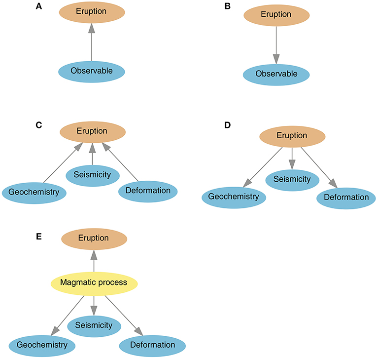
Figure 1. Simplified examples of model structure to forecast volcanic eruption; parts (A–D) model the relation of observables and eruption; for (A,B), there are only two nodes, “Eruption” and “Observable,” which are dependent; for (C,D) the observable node is split into “Geochemistry,” “Seismicity” and “Deformation”; in (C) the observables are independent and in (D) they are dependent on eruption and independent of each other, given eruption. Panel (E) is an example of a causal BN, where “Magmatic process” is the parent node for “Eruption” and the observables. “Eruption” and the observables are conditionally independent given “Magmatic process.” The model is a simplification of the La Soufrière model (Hincks et al., 2014) that we adapted to our pilot study.

A BN model structure, and quantitative information about the variables, can be retrieved either from data, when available, or from experts, or a combination of both. BNs are applied in many different domains (e.g., Pourret et al., 2008; Weber et al., 2012), including risk assessment decision support (e.g., Aspinall et al., 2003; Fenton and Neil, 2013; Gerstenberger and Christophersen, 2016).

When implemented as a software program, a BN allows easy but rigorous quantification of the strengths of relationships between different variables. Moreover, the implementation of Bayes' rule (Bayes and Price, 1763), within the program, allows probabilities to be updated in the light of new evidence. Thus, a BN can be used to evaluate formally a variety of different “what if” scenarios in the face of substantial scientific uncertainties: it is this capability that makes the BN framework an invaluable decision resource for supporting volcano forecasting.

Developing the Model Structure

Developing the model structure involves defining the variables and identifying possible parent-child relationships. Figure 1 illustrates different simplified modeling options for a volcanic eruption. For examples Figures 1A,B have only two nodes, “Eruption” and “Observable” (e.g., seismicity), while the other examples split the observables into “Geochemistry,” “Seismicity” and “Deformation.” In these examples, there are correlations between some of the nodes, but this does not imply causation—the observable does not cause the eruption, nor does the actual eruption event itself cause the precursory unrest. There are, however, internal processes that lead to eruption, which also cause observable precursory phenomena.

With these elemental examples in Figures 1A–D, the arcs can point either direction; in reality, however, there will be internal processes, such as ascending magma or a magmatic perturbation of the hydrothermal system, that involve underlying latent causal links between precursory observables and eruption. For example Figure 1E is a simplification of the model by Hincks et al. (2014) developed to retrospectively analyze the 1975–1977 volcanic crisis at La Soufrière volcano, Guadeloupe. Here, the node “Magmatic process” is the parent node of the eruption and of the observable nodes and thus the model represents cause-and-effect relationships. Generally, the structure depends on data availability and the quantification requirements as further discussed in the next section.

Quantifying the Model

The information required to quantify a BN model depends on the type of variable represented by each node. Commonly variables have a finite number of states that are mutually exclusive, and discrete values exhaustively describe these possible node states. For such variables, the dependencies are captured in Conditional Probability Tables (CPTs), as illustrated with our simple examples (Figure 2 and further explained below).

FIGURE 2

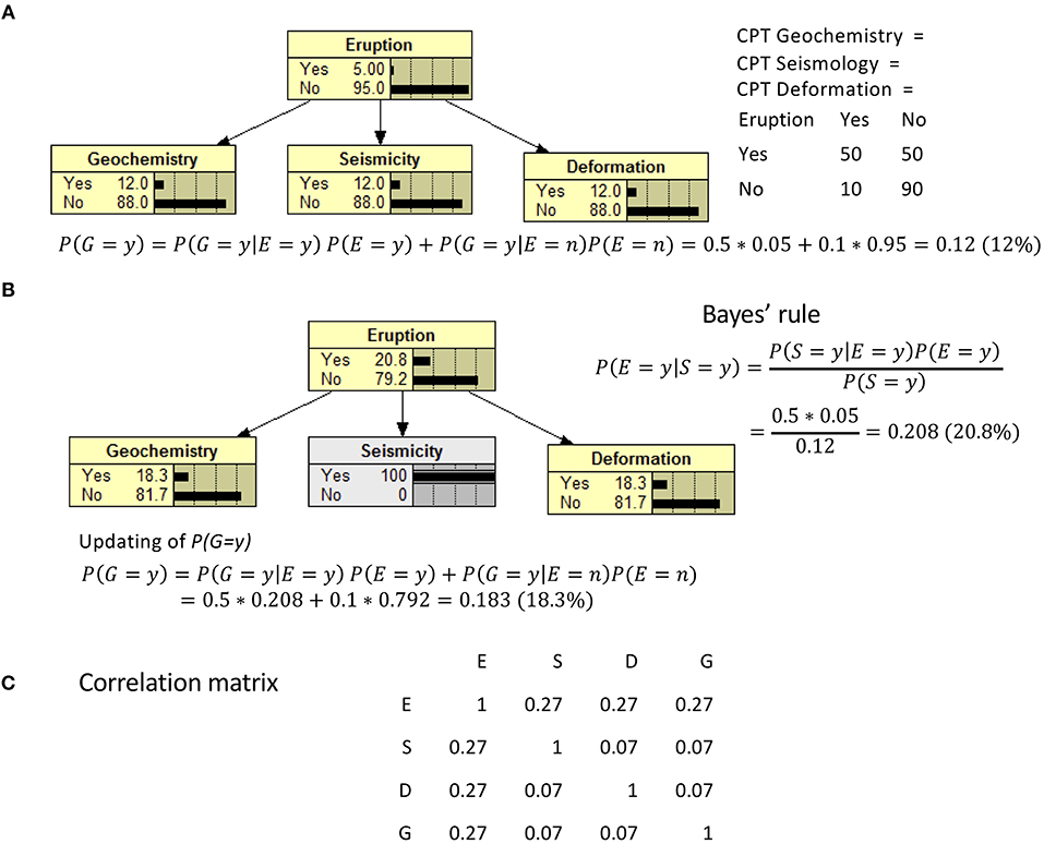
Figure 2. An illustration of the BN calculations for Figure 1D. We assume a monitoring period of 1 month. The probability of Eruption in any 1 month is 5%. The CPTs for all observables are assumed to be the same in this simple example and the probability of each observable is assumed to be 50% if an Eruption occurs and 10% otherwise. The calculation of the probability for the observables is given for Seismicity in (A). In (B), Seismicity is observed, and the probability of Eruption is updated according to Bayes' rule. Given a new probability for Eruption due to an affirmative observation of Seismicity, probabilities for Geochemistry and Deformation are also updated because they are conditionally dependent on Eruption state probability (the revised Bayes' calculation is given for the Geochemistry node). Panel (C) shows the correlation matrix of the variables from 100,000 simulated cases.

However, when variables are best characterized by continuous values, the most common approach (apart from asserting some form of discretization) is the assumption of a parametric joint distribution, most often the joint normal distribution. To quantify such models one needs conditional means and variances for the nodes, and regression coefficients for the arcs (Pearl, 1988; Shachter and Kenley, 1989). Unfortunately, often the assumption of joint normality is not validated in practice. Other modeling techniques for continuous variables exist (Hanea et al., 2006; Langseth et al., 2009). In volcanology, the type of probability distribution for a given variable is often unknown, due to data scarcity, and several distributions may seem plausible (Tierz et al., 2016a,b). Alternative distributions could be tested within a BN framework.

For a discrete BN, as in Figure 1A, we need to assess the marginal probability distribution of the variable “Observable.” For the variable “Eruption,” we need to know the probability of “Eruption,” given the state of “Observable.” In the simplest case, each node has two states, “yes” or “no.” Even though there are only two possible outcomes for “Eruption,” the model is still probabilistic, since it calculates the probability of either “yes” or “no.” To quantify the prior table for the “Observable” node (O), it is sufficient to assess one probability value, P(O = yes) or P(O = no), because given the mutually-exclusive-and-exhaustive requirement: P(O = yes) = 1 − P (O = no), and vice versa. For the same reason, to quantify the CPT of the “Eruption” node (E), given the “Observable” node (O), we only need to assess two probability values, because: P(E = yes|O = yes) = 1 – P(E = no|O = yes) and P(E = yes|O = no) = 1 – P(E = no|O = no). By the law of total probability, the probability of “Eruption” can then be calculated, using simple probability rules, to be P(E = y) = P(E = y|O = y)*P(O = y)+ P(E = y|O = n)*P(O = n). Eruption could have several states E1, E2, E3, and E4 distinguishing different eruption styles (e.g., Hincks et al., 2014). In that case, the probabilities to be assessed are P(E1|O = y), P(E2|O = y), P(E3|O = y) and P(E4|O = y), where again one probability can be calculated using the other three because the sum of all four must be one, since the states are mutually exclusive and exhaustive. Additionally, the probabilities P(E1|O = n), P(E2|O = n), P(E3|O = n) and P(E4|O = n) must be assessed.

In case Figure 1B, we need to assess the probability distribution of the variable “Eruption,” i.e., for the two states E = y and E = n, we need the probabilities P(E = y) and P(E = n), which must add up to one. For the node “Observable,” we need the conditional probability depending on the states of “Eruption.” So, in the above example, the questions to answer are “what is the probability of observing unrest seismicity given an eruption subsequently occurs?” and “what is the probability of observing unrest seismicity given no eruption occurs?”

The required number of probabilities for a node increases with the number of parent nodes and the number of states of both parent and child node. While there is little difference in assessing the probabilities for cases (Figures 1A,B), this changes when comparing the probability estimates required for cases (Figures 1C,D), which both have three observables “Geochemistry,” “Seismicity” and “Deformation.” In case Figure 1C we need to assess the marginal distribution of each of the observable nodes, similar to case a). Additionally, we need to assess the probability of eruption given all possible combinations of its parents' states. If each of three parent nodes has two states, the number of combinations is 2³ = 8. Quantification quickly becomes intractable as the number of nodes increases and nodes have more than two states. Some parent state combinations may happen extremely rarely, engendering large uncertainties. In contrast, the complexity of the probability assessment in case (Figure 1D) compared to case (Figure 1B) has not changed.

The construction and the quantification of BNs are interrelated, and the chosen structure may change depending on the quantification requirements, data availability, and/or the understanding and representation of the problem. Different modeling choices come with advantages and disadvantages. Using joint normal distributions that preserve the properties of continuous value variables precludes representation of marginal distributions with heavy tails, or tail dependence, as part of the dependence structure. Complex dependence structures may be better represented using large CPTs by discretizing continuous variables into a large number of states. However, this comes with the price of a huge quantification burden, which, in the absence of massive data sets, renders poorly quantified conditional distributions. A mentioned above, data may be unavailable to fully or even partially quantify a chosen BN. When data are absent or incomplete, expert elicitation can contribute to BN quantification.

Structured Expert Judgment

Structured expert judgment (SEJ) is the process of eliciting expert knowledge as a form of scientific data (Colson and Cooke, 2017). A variety of expert elicitation protocols have been developed over recent decades, and successfully deployed in numerous domains (O'Hagan et al., 2006; Cooke and Goossens, 2008; Aspinall, 2010; Selva et al., 2012; Hanea et al., 2016). Most follow thoroughly documented methodological rules, but they differ in several aspects, including the way interaction between experts is handled, and the way an aggregated opinion is obtained from individual experts. There is no single, best SEJ protocol: each has strengths and weaknesses.

There are two main ways in which experts' judgments are aggregated: behaviorally, involving striving for consensus via discussion and deliberation (e.g., O'Hagan et al., 2006), and mathematically, involving independent individual expert estimates being combined with a given mathematical rule (e.g., Cooke, 1991). Mathematical rules provide a more explicit, auditable and objective approach. A weighted linear combination of opinions is one example of such a rule. Equal weighting is often used, mostly because of its simplicity. While evidence shows that equal weighting frequently performs well relative to more sophisticated aggregation methods for reliably estimating central tendencies (e.g., Clemen and Winkler, 1999), when uncertainty quantification is sought, performance-based weighting provides superior information (Colson and Cooke, 2017).

One accepted differential weighting scheme is the Classical Model for SEJ (Cooke, 1991). Perhaps its most distinguishing feature is the use of calibration variables to derive performance-based weights, providing an empirical basis for validating experts' judgments. Calibration (or “seed”) variables are taken from the problem domain for which, ideally, true values become known post-hoc (Aspinall, 2010). However, this is rarely feasible in practice and so calibration questions with known realizations (values) are used instead. Experts are not expected to know these values precisely, but they are expected to be able to capture them within informative ranges, defined by ascribing suitable values to marker quantiles (e.g., 5, 50, and 95th percentiles). The Classical Model has been the SEJ method most frequently applied for volcanic hazard and risk assessment worldwide, for many years (Aspinall, 2006; Martí et al., 2008; Neri et al., 2008; Wadge and Aspinall, 2014; Bebbington et al., 2018). As a consequence, many volcanologists are familiar with the approach and associated procedures.

Nevertheless, it is challenging to find calibration questions that closely match the types of questions needed to elicit conditional probabilities for a BN, especially if there are no analogs from real-life observations. For our pilot study, we did not have the resources to develop appropriate seed questions. We used SEJ with average weighting of experts, and introduced the concept of calibration to the participating experts for possible future applications.

Benefits of BN Modeling Within and Beyond the Pilot Study

Behind the intuitive visualization of a complex relational problem, which allows collaborative drafting and quantification of models, the most palpable advantage of a BN is its rigorous probabilistic foundation. BNs offer a flexible platform and can easily combine expert input, incomplete data sets, and other disparate sources of information. For example, different expert panels can contribute sub-models, which can then be combined to represent a complex system. If partial data sets are available, the sub-models' parameters can be fitted from data. When suitable data sets are available, entire sub-models (the structure and parameters) can be learned from data, using machine-learning techniques (Murphy, 2012), potentially extending and complementing expert knowledge.

Once the BN is built and fully quantified, its main use is to update distributions given new data or additional observations. This is referred to as instantiation, inference, or (less commonly) bi-directionality (Gerstenberger et al., 2015). Evidence added to one node will change the probabilities of all dependent nodes, regardless of the direction of the arcs. This is illustrated in Figure 2, which uses the elemental example of Figure 1D. We assume a monitoring period of 1 month. The probability of “Eruption” in any 1 month is assumed to be 5% as shown in Figure 2A. If an Eruption occurred, we assume that any precursory variable was observed in 50% of the prior months. The probability of any of the observations is 10% in a month when no Eruption occurs the following month as shown in the CPTs in Figure 2A. If “Seismicity” is observed, Bayes' rule can be applied to update the probability of “Eruption.” Given an increased probability of “Eruption” the probabilities of the dependent nodes “Geochemistry” and “Deformation” also increase. It may seem counterintuitive that the observation of “Seismicity” has any impact on the probabilities of seeing changes in other observables. However, the BN has implicit connections between observable nodes via hidden processes relating to “Eruption.” The CPTs express these dependencies which, in the real world, are driven by underlying magmatic processes that are not directly modeled in this variant of a BN model. Figure 2C shows the correlations between the four variables in the BN model. We used the BN software Netica (Norsys, 1995-2018) to simulate 100,000 realizations of the joint distribution of the four variables. We calculated these correlations to illustrate that dependence through correlations may result from the chosen CPT values despite the lack of causal relation between these variables.

The bi-directionality of BNs is a large advantage over event trees: BNs can be used to analyze the dependencies and can advance the understanding of the system. This characteristic can also be beneficial in operational applications; for example, if one loses seismograph network coverage due to a telecommunications signal failure, the BN allows one to infer what the likely seismicity level would be, given other non-seismic observations. Even more important, the BN allows one to make use of “negative evidence”: if gas flux suddenly decreases, is it due to a conduit blockage (dangerous) or to a change in gas exsolution in the reservoir (likely benign)? The two carry quite different hazard implications, and both scenarios need to be accommodated and ascribed relative probabilities. Inference as to which is the actual cause may be weighed by what other observables are indicating.

Pilot Study of a Discrete BN Model to Forecast Eruptions on Whakaari/White Island

This section provides some background on volcano monitoring in New Zealand before describing Whakaari/White Island, the volcano chosen for the pilot study. We briefly outline the motivation for the pilot study before describing pilot model structure, the estimated probabilities and the eruption probabilities. We briefly discuss other findings from the workshop and close with a demonstration of typical BN calculations for two individual experts.

Volcano Monitoring in New Zealand

In New Zealand, GNS Science, through the GeoNet project, conducts national volcanic monitoring (New Zealand Ministry of Civil Defence Emergency Management, 2015). GeoNet issues notifications of any change in volcanic alert level status through Volcanic Alert Bulletins to the Ministry of Civil Defense and Emergency, other agencies, and the media. Volcanic Alert Bulletins are also published on GeoNet's website (GeoNet, 2018).

GeoNet coordinates the volcano monitoring team, which consists of GNS Science staff based at three sites. The volcano monitoring team meets regularly to review the status of all 12 monitored New Zealand volcanic centers, and to set Volcano Alert Levels (Potter et al., 2014) and the Color Codes of the International Civil Aviation Organization. Team members prepare Volcanic Alert Bulletins when required. The team is responsible for providing scientific advice to emergency management authorities at the national, regional, and local level (New Zealand Ministry of Civil Defence Emergency Management, 2015). In addition to these legislative requirements, the volcano monitoring team regularly estimates the probability of forthcoming eruptions for internal health and safety policy requirements (Jolly et al., 2014; Deligne et al., 2018).

GeoNet data is available free of charge. While GeoNet is committed to transparent data discoverability, the process of operationalizing data discovery for non-continuous data (e.g., monthly gas flights, gas isotope sampling results) was in its early stages at the time of our pilot study, and therefore not readily available for the model development. Thus, the parameters of the BN model were estimated by expert elicitation rather than from data.

Whakaari/White Island Volcano

Whakaari/White Island volcano is of one New Zealand's most active volcanoes and it is a major tourist attraction. Located about 50 km off the coast of the North Island (Figure 3), it is the northernmost subaerial active volcano of the Taupo Volcanic Zone (Cole and Lewis, 1981). Its emerged area of 3.3 km² is the summit of the much larger White Island Massif (Cole and Nairn, 1975). The volcano is andesitic to dacitic in composition and is formed of two overlapping cones with a succession of lava flows, breccias, agglomerates, and unconsolidated beds of ash and tuffs containing lava blocks (Black, 1970). Its main topographical feature (Main Crater) consists of three sub-craters: western, central and eastern (Houghton and Nairn, 1989, 1991), with the current active vent in the eastern sub-crater.

FIGURE 3

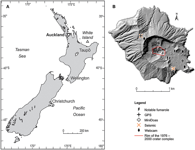
Figure 3. (A) Map of Whakaari/White Island's location in New Zealand and (B) map of Whakaari with position of notable features and GeoNet monitoring equipment.

Figure 4 illustrates a conceptual model of the volcano. The magmatic system is perceived to consist of a deep collective reservoir (4–7 km) that feeds a shallower convective reservoir (1–2 km) from which small amounts can be injected into an upper conduit to the surface (Clark and Otway, 1989; Houghton and Nairn, 1989; Cole et al., 2000; Kilgour et al., 2016). Werner et al. (2008) proposed that gas and magma are transported from deep to shallow levels within a closed system (magma convection), while an open system characterizes the upper conduit. Steaming ground areas, hot springs, fumaroles, and an acidic crater lake are the surface expressions of the volcano hydrothermal system which has existed for at least 10,000 years (Giggenbach and Glasby, 1977). Several attempts have been made to characterize the volcano's hydrothermal system (e.g., Ingham, 1992; Nishi et al., 1996a). From the location of volcanic earthquakes, Nishi et al. (1996b) suggested that the active hydrothermal system is located below Main Crater but its extent and evolution with time (e.g., presence of a seal) remain poorly understood. The Crater Lake level had several filling/evaporative cycles that correlate with varying discharge of the springs (Christenson et al., 2017).

FIGURE 4

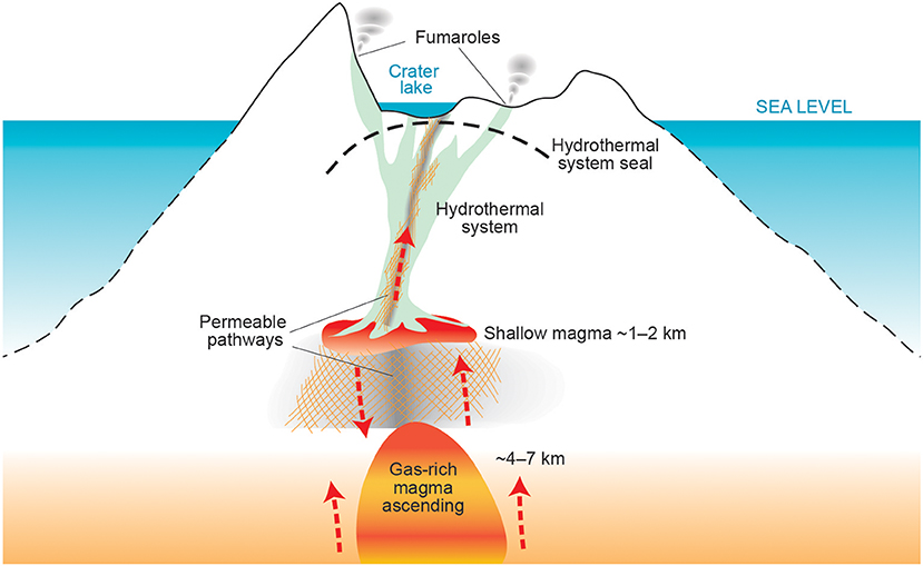
Figure 4. Conceptual model of Whakaari volcano capturing the variables that are modeled in the BN, including two magma reservoirs, the hydrothermal system and the crater lake. Note that this is not to scale.

Volcanic activity ranges from fumarolic and hydrothermal during quiescence, to phreatic, phreatomagmatic, Strombolian and effusive during more active periods (Cole and Nairn, 1975; Houghton and Nairn, 1989; Nishi et al., 1996b; Chardot et al., 2015). A major eruptive magmatic episode occurred between 1976 and 2000 and formed the current active crater (Figure 3); this episode comprised several cycles, with intra-episode clusters of activity from 1976 to 1993, 1998, 1999, and 2000. There were at least 250 eruptions during this quarter-century period, ranging from localized steam and mild ash eruptions to eruptions with ejecta outside the Main Crater (G. Jolly, personal communication). These eruptions are not classified by eruption style, but 45 had ballistic and/or surge impacts beyond the crater complex (Figure 3B), suggesting an eruption rate of 0.15 large eruptions/month. Assuming a Poisson distribution for the number of eruptions in a month, the probability of one or more eruptions within 1 month can be calculated from the rate R like 1-exp(-R). Thus, the probability of one or more eruptions within 1 month impacting beyond the 1976–2000 crater complex is 14%. However, the 1976–2000 eruptive episode altered the volcanic system and the prior rate is not necessarily representative of activity since.

The most recent eruptive episode began with unrest in August 2011 (Chardot et al., 2015), and continued through the end of 2016. During this episode there were eight eruptions (Table 1), half of which had ballistic and/or surge outside the 1976–2000 crater complex and would have posed safety concerns if they had coincided with site visits to the island. Calculating an average rate of eruptions impacting beyond the crater rim for the period from 2001–mid 2018, there were four eruptions within 210 months, which equals 0.02 per month. The Poisson probability for an eruption within 1 month impacting beyond the 1976–2000 crater complex is 2%. There was also one magmatic effusive eruption in form of a lava dome (Table 1). There were no eruptions in the 2 years leading up to the expert elicitation workshop central to our pilot study.

TABLE 1

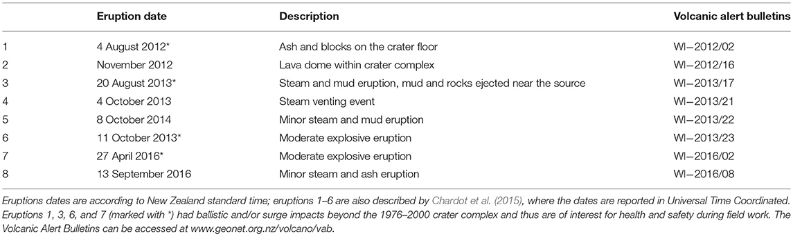
Table 1. The dates and description of the eight eruptions of Whakaari's most recent eruptive period from 2012 to 2016.

Eruptions at Whakaari can be preceded by increased levels of seismicity (Latter et al., 1989), magnetic changes (Hurst et al., 2004) and deformation within Main Crater (Clark and Otway, 1989), although eruptions can occur with no useful short-term precursory activity to indicate that an eruption is imminent. In the case of the examples cited, changes in monitored parameters were observed months before the eruption.

Volcano monitoring at Whakaari has been ongoing since 1967 and part of the GeoNet project since its inception in 2001. As of August 2018, monitoring includes continuous visual observations (three on-island webcams), seismic (two continuous seismic broadband stations), deformation (two GPS stations) and SO₂ emission measurements (two miniDoas sites) (Figure 3B), with additional monthly gas flights (CO₂, SO₂, and H₂S emissions) and regular field campaigns (e.g., leveling, fumarole and spring sampling, CO₂ soil gas surveys, magnetic surveys).

Whakaari's seismicity presents a full spectrum of event types, ranging from long-period to volcano-tectonic events and tremor (Sherburn et al., 1998). However, the limited number of local seismometers (and the nearest station off the island being about 50 km away) prevents the accurate and precise location of local seismic events. Therefore, we can determine the depths of larger earthquakes that are recorded off island but have little or no effective depth control on the more frequent small events.

Deformation is mainly assessed using campaign-leveling data, and the sources of the recent changes are interpreted as being due to varying pressurization of the main fumarole field (Peltier et al., 2009; Fournier and Chardot, 2012; Christenson et al., 2017).

Motivation for the Pilot Study

The pilot study was motivated by a GNS Science internal presentation on life safety when working on volcanoes. At GNS Science, thresholds of 10⁻³, 10⁻⁴, or 10⁻⁵ for the hourly probability of a fatality at an active volcano trigger different levels of managerial sign-off for undertaking fieldwork on the volcano (Jolly et al., 2014; Deligne et al., 2018). As input to the life-safety risk calculations, members of the volcano monitoring team regularly estimate the probability of an eruption for New Zealand volcanoes in a state of unrest. Small probabilities are challenging to estimate (Burns et al., 2010), and the team has no shared quantitative tools or models to assist with determining the eruption probabilities. This is in contrast to the GNS seismology team that has several models to forecast earthquake occurrence on different time scales (Christophersen et al., 2017); the latter are being continuously tested and evaluated in international testing centers (e.g., Gerstenberger and Rhoades, 2010; Rhoades et al., 2016). Recent positive experience with BN modeling for risk assessment in carbon capture and storage (Gerstenberger and Christophersen, 2016) motivated us to explore BNs to address volcanic eruption probabilities.

Our goal was not to develop the first operational BN model for eruption forecasting in New Zealand, but to explore the utility of BN modeling for eruption forecasting in principle, and to investigate the challenges and potential benefits of the method. As a consequence, we were experimental in out approach. For example, we did not attempt to constrain the number of variables to a manageable number, quite the opposite; for the first model, we aimed to capture all variables that are regularly monitored. We also did not insist on consistent definition of all nodes, as further explained below.

Pilot Model Structure

The aim of the model is to capture the conceptual understanding of the volcanic processes that lead to eruptions and to represent all regularly monitored observables. The pilot BN did not attempt to model dynamic or transient aspects of the volcanic system, such as potential drying of the crater lake, which would engender substantive changes in some variables. The development of the model structure was iterative and involved defining the variables. It took a 2-h meeting for a small team with diverse skill sets to adapt the La Soufrière model to Whakaari and two further hours to draft the initial set of elicitation questions. Ideally there would have been two to three 2-h meetings with a small group of experts from different sub-disciplines to review and fine-tune sub-networks for the overall model. Having a working BN model example (Hincks et al., 2014) helped participants who were new to BN modeling, enabling them to quickly grasp the concepts and understand what we were trying to achieve.

Through feedback with individual experts, we quickly ascertained that individuals from different sub-disciplines had different understandings of the eruption driving processes. As a consequence, several node definitions were purposefully left vague to accommodate different thinking about these processes. A joint discussion with experts from seismology, fluid geochemistry, geodesy, and general geophysics highlighted how the BN framework allowed the different understandings of the volcanic processes to be discussed in an insightful way. Unfortunately, the pilot study had time constraints that did not allow full agreement to be reached on all the nodes.

Figure 5 presents an overview of all nodes that were elicited. The model structure follows Figure 1E, where observables are conditionally independent of eruption given magmatic processes. For ease of handling, we split the model into four areas during the model development process and the expert elicitation. The areas, described in more detail below, are: (1) volcanic processes leading to eruption, (2) observations related to seismicity, (3) observations related to surface manifestations, and (4) fluid-geochemical observations. Table 2 summarizes the nodes describing the volcanic processes leading to eruption and the eruption nodes.

FIGURE 5

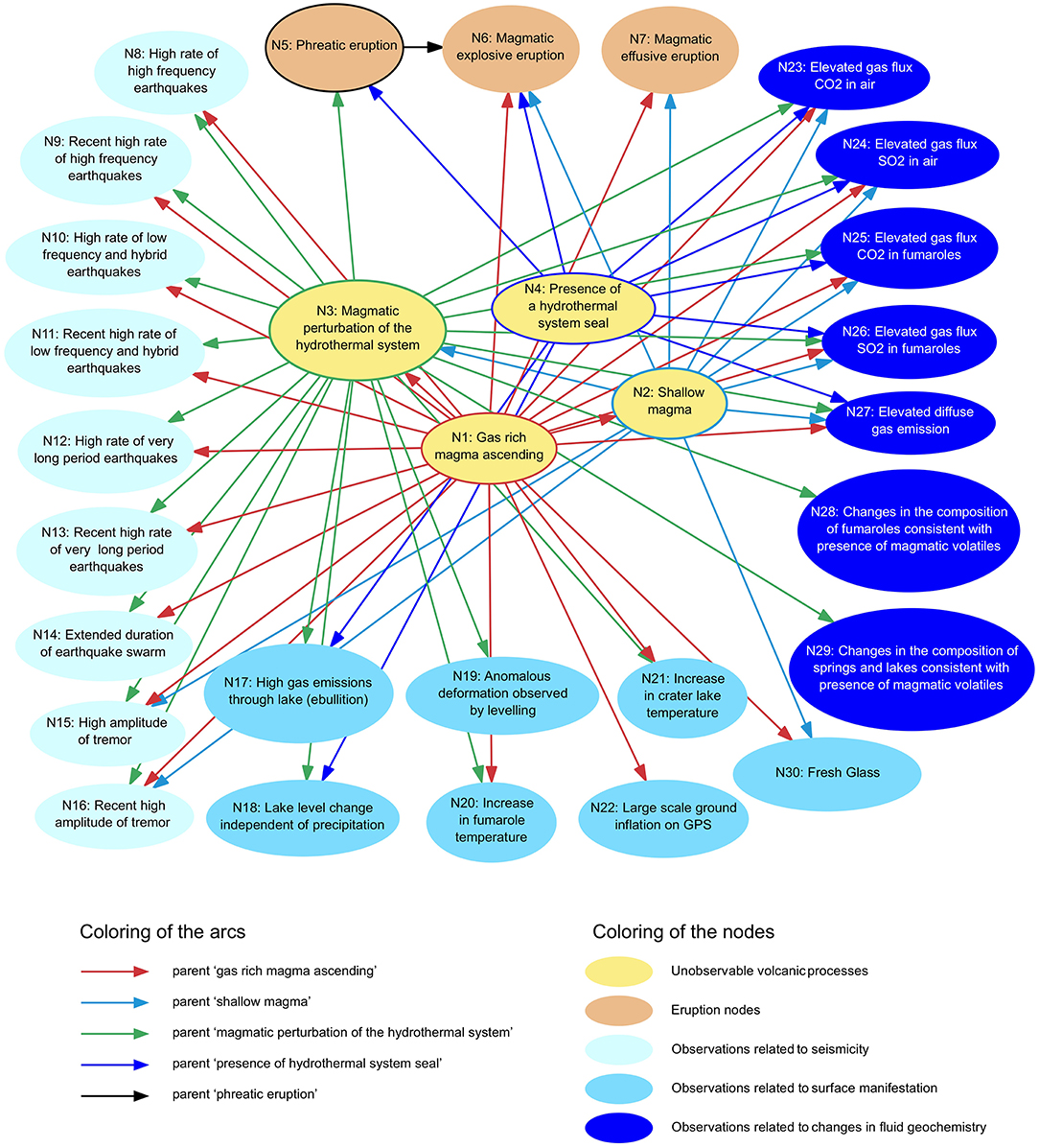
Figure 5. The model structure of the BN to forecast volcanic eruption on Whakaari in the next month; see legend for explanation of arrow and node colors.

TABLE 2

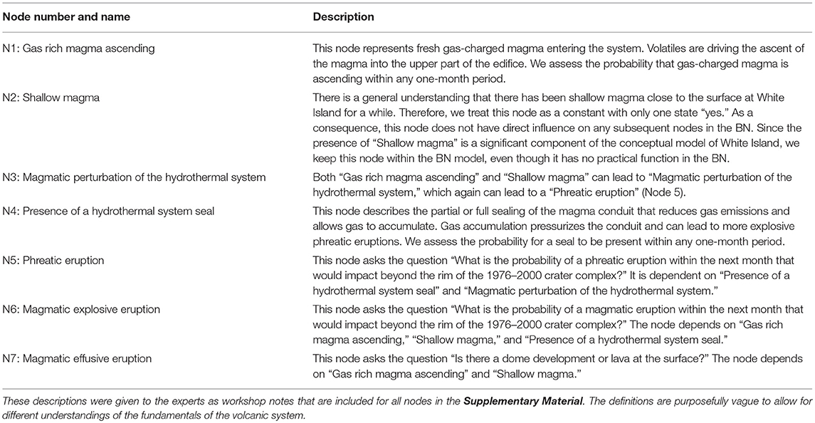
Table 2. The description of nodes 1–4 that capture the hidden processes of the volcano and nodes 5–7 that model three types of eruption.

Volcanic Processes Leading to Eruption

The model simplifies the volcanic processes that can lead to eruption into four unobservable nodes (yellow ovals in Figure 5). Node 1 is “Gas rich magma ascending” and represents fresh gas-charged magma entering the system from depth. Volatiles are driving the ascent of the magma into the upper part of the edifice. Node 2 is “Shallow magma” and represents the presence of a shallow magma reservoir being fed by the deeper reservoir. “Gas rich magma ascending” can fill the shallow magma reservoir and therefore is a parent of “Shallow magma.” There is consensus that there has been shallow magma close to the surface at Whakaari for at least several decades (Houghton and Nairn, 1989; Cole et al., 2000). Therefore, we treat this node as a constant (state “yes”). As a consequence changes in its parent or child nodes have no direct influence on the node itself or on other dependent nodes. However, since the presence of “Shallow magma” is a critical component of the conceptual model of Whakaari (Figure 4), we chose to keep this node within the model. Node 3 is “Magmatic perturbation of the hydrothermal system.” Both “Gas rich magma ascending” and “Shallow magma” can lead to “Magmatic perturbation of the hydrothermal system.” Node 4 is “Presence of a hydrothermal system seal,” which has no parents. This node describes the partial or full sealing of the hydrothermal system seal that reduces gas emissions and allows gas to accumulate. Gas accumulation pressurizes the conduit and can lead to more explosive phreatic or magmatic explosive eruptions.

The volcanic processes can lead to three types of eruption (orange ovals in Figure 5): “Phreatic eruption” (node 5), “Magmatic explosive eruption” (node 6) and “Magmatic effusive eruption (node 7). Phreatomagmatic eruptions are included in magmatic explosive eruptions. The La Soufrière model only had one eruption node with different states for different eruption types. We struggled to define mutually exclusive and exhaustive states because different eruption types can occur within the 1-month period of interest. We explored the option of estimating the probability of the next eruption within the 1-month period but found it easier to represent different types of eruption by separate nodes. To be consistent with the regular elicitation of eruption probabilities, nodes 5 and 6 are defined as one or more eruptions within the next month “impacting beyond the rim of the 1976–2000 crater complex” (see Figure 3). A magmatic effusive eruption (node 7) includes dome development and any lava at the surface. It is likely to happen within the crater, which is at a lower elevation than the area the monitoring team would access. Historically, lava domes at Whakaari are small in comparison to other volcanoes and are therefore not an immediate threat to health and safety during fieldwork. Figure 5 shows how the eruption nodes are connected to the driving processes.

Observations Related to Seismicity

Observations related to seismicity include three types of earthquake occurrence distinguished by their frequency content, and tremor. They reflect the variety of events recorded at Whakaari (Sherburn et al., 1998). The reader is directed to the review by McNutt (2005) for a comprehensive description of each earthquake type. For each of these observables there is an additional node that captures recent occurrence of the respective observables and reflects that the system may have a memory. Thus, recent activity can indicate that fluids or magma have shifted in the system. Here, we only discuss the main process(es) driving each type.

High frequency earthquakes (node 8 for high rate and node 9 for recent high rate) are associated with shear fracture and thus an indication of stress changes. Low frequency and hybrid earthquakes (node 10 for high rate and node 11 for recent high rate) are thought to be associated with fluid processes. Very long period earthquakes are associated with significant fluid movement in the subsurface (node 12 for high rate and node 13 for recent high rate). A further node “Extended duration of earthquake swarm” (node 14) assesses the duration of earthquake activity. We do not distinguish the frequency content of the earthquakes that contribute to the swarm because it may be difficult to measure the frequency content when more than one process is causing the earthquake occurrence. We also consider tremor, which is a persistent seismic signal of varying durations often associated with volcanic eruptions (Konstantinou and Schlindwein, 2003 and references therein). High amplitude of tremor (node 15 for high amplitude and node 16 for recent high amplitude) can reflect the size of an eruption, following McNutt (2005), who showed that higher tremor amplitudes correlate with higher Volcanic Explosivity Index of eruptions. At Whakaari, periods of increasing tremor have been modeled to retrospectively forecast eruptions (Chardot et al., 2015).

All of the nodes representing observations related to seismicity (nodes 8–14) have the same two parents: “Gas rich magma ascending” and “Magmatic perturbation of the hydrothermal system.” The tremor nodes (nodes 15 and 16) also depend on “Shallow magma.”

Observations Related to Surface Manifestations

This part of the model considers the nodes related to deformation and to the crater lake and the temperature of fumaroles. “Anomalous deformation observed by leveling” (node 19) has, as parent, the “Magmatic perturbation of the hydrothermal system” and “Large-scale ground inflation as measured by GPS” (node 22) has as parent the node “Gas rich magma ascending.” “High gas emissions through lake (ebullition)” (node 17) and “Lake level change independent of precipitation” (node 18) have as parents the “Magmatic perturbation of the hydrothermal system” and the “Presence of a hydrothermal system seal.” “Increase in fumarole temperature” (node 20) and “Increase in crater lake temperature” (node 21) have the parents “Gas rich magma ascending” and “Magmatic perturbation of the hydrothermal system.”

One node, “Fresh glass” (node 30), was added during the elicitation workshop and has as parents the “Gas rich magma ascending” and the “Shallow magma” nodes.

Observations Related to Changes in Fluid Geochemistry

Elevated gas emissions usually relate to elevated volcanic activity (e.g., Giggenbach and Sheppard, 1989). Observations related to changes in fluid geochemistry include “Elevated gas flux of CO₂ in air” (node 23), “Elevated gas flux of SO₂ in air” (node 24), “Elevated gas flux of CO₂ in fumaroles” (node 25), “Elevated gas flux of SO₂ in fumaroles” (node 26) and “Elevated diffuse (soil) gas emission” (node 27).

“Changes in the composition of fumaroles consistent with the presence of magmatic volatiles” (node 28) and “Changes in the composition of springs and lakes consistent with the presence of magmatic volatiles” (node 29) are also indications of “Gas rich magma ascending.” However, the change of the composition would be fed into the fumaroles through the hydrothermal system. Only in case of very high temperature fumaroles (≥800°C) would the hydrothermal system be circumvented (Giggenbach and Sheppard, 1989). Therefore, the experts decided that only “Magmatic perturbation of the hydrothermal system” is a parent of these two observable nodes (28 and 29).

Definitions of States

Clearly defining the nodes and states—so that all experts share the same understanding of the elicitation questions—is an important part of the BN model development. To reduce the elicitation burden we described each variable with two states only: “yes” and “no.” Since the probabilities for all states must add to 100%, we only asked the question for the “yes” state and calculated the complementary “no” state probability. During the model development, experts voiced strong reservations about defining variables with hard, definite thresholds. They were concerned that one or more variables might be significantly elevated, such as seismicity prior to the 2014 deadly Mount Ontake eruption (Kato et al., 2015), but still not reach the threshold set to trigger a warning. Near-misses against arbitrary threshold for node states can also lead to negative (Brier) skill score which appear to devalue BN forecast performance, as was found for Soufrière Hills Volcano, Montserrat (Wadge and Aspinall, 2014). Experts in our study wanted to model the observables as continuous probability density function. While the modeling techniques we could access during the pilot model study did not allow for this, we envisaged continuous BN modeling as subsequent model development. As a consequence, we did not define thresholds for the states of the observable nodes because experts had widely varying opinions on what levels are appropriate. Attempting to enforce consensus on issues about which our experts had strong reservations seemed counter-productive to the aim of the study, which was to explore the utility of BN modeling for eruption forecasting in New Zealand.

Instead we asked each expert during the quantification of the model to describe what threshold they had in mind when answering the question. For example, for node 8 “High rate of high frequency earthquakes” we asked, “how do you define “high rate” of high frequency earthquakes?” There is a wide variation in the definitions of thresholds, and for node 8 the answers were: More than 5,10, 20, 30 (two experts), 50, 100 per day, more than two times the background; one magnitude greater than the background rate; a couple of earthquakes per hour for at least half a day, visible with the naked eye on the seismogram. In another example, for node 20, the answers to “how do you define an increase in fumarole temperature” were: + 5°C, +10–15°C, +10–20°C, +20°C (three experts), +10% of past value, more than 20% change from recent trend, 2–3 times the normal temperature. For node 22, “How do you define elevated gas flux of CO₂ in air” the answers were: More than 250, 500, few hundred, 1,000, 2,000, 2,000, 3,000 tones/day; at least two measurements more than 20% above baseline, increase by over 100% over the background value. Having different thresholds for the states of the observable nodes limits the usability of the pilot study. Although theoretically possible, we did not attempt to group similar answers and use the matching probability estimates to derive a BN with consistent state, because the experts had reservations about using a model with only two states for the observable nodes.

The Estimated Probabilities

To quantify the model, the experts estimated 120 probabilities and their 80% confidence intervals, which are summarized in Christophersen (2017). Figure 6 presents a few questions to show the spread in answers between experts. Broadly, the elicitation questions can be split into four categories depending on the overlap of the experts' uncertainty intervals. Figure 6a shows an example of good agreement, where all experts' ranges overlap. Figure 6b is an example in which the uncertainty range of one or two experts fell outside the rest of the answers. In Figure 6c the experts' answers fell into two groups with some overlap of the uncertainty range, which indicates large uncertainty in the answer. Finally, Figure 6d is an example of even larger uncertainty, because the variety of answers covers the entire possible range (from 0 to 100%) and individual ranges tend to be wider. Experts are in good agreement for only 22 out of 120 questions.

FIGURE 6

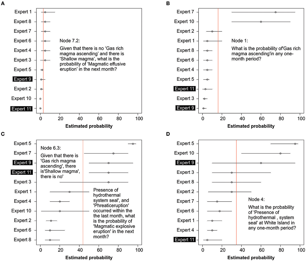
Figure 6. Examples of probability range graphs of the 11 experts and their averaged median values (vertical red line) for four nodes, which show: (A) a node with good agreement of experts' judgments; (B) two apparent outlier credible intervals; (C) two groupings of experts' judgments, and (D) large uncertainties in experts' credible intervals. For each graph the experts' ranges are ordered in terms of decreasing median size and thus the numbering on the y-axis does not refer to the same expert in the different examples.

For about one third of the questions (43 out of 120), there are one or two experts who answered significantly differently to the others. This may be because they understood the questions differently, or they had different definitions of states in mind. Alternatively, they might have a different understanding of the system or its processes. With more time and resources, it would have been beneficial to explore these outliers as they could help improve model definitions. For about half the questions, there were either two dichotomous groups of responses (17 out of 120), or a very large spread of values (38 out of 120). Thus, for about half the questions there were large uncertainties in the probability estimates.

The Eruption Probabilities

The eruption probabilities are a main result from the pilot modeling and are shown in Figures 7, 8. The nodes that are relevant for calculating the eruption probabilities are the four unobservable nodes (yellow ovals in Figure 5) and the three eruption nodes (orange ovals in Figure 5). These nodes had the same definition of states for all experts and therefore we present the results for each individual expert as well as combined results. Combining experts' judgments becomes problematic only if we wish to condition on any of the observables of the BN (nodes 8–30); this is because then different thresholds, chosen by the experts, would come into play.

FIGURE 7

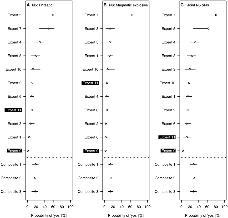
Figure 7. The probabilities of different hazardous eruption styles in the next month: (A) node N5: Phreatic eruption; (B) node N6: Magmatic explosive eruption, and (C) the joint probability of N5 and N6. Each graph shows the probability for an eruption in the next month sorted by the 50th percentile for the 11 individual experts and for three composite results. Please see text for an explanation of the three composite results.

FIGURE 8

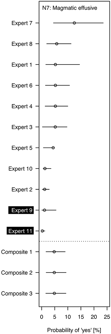
Figure 8. The probability of a magmatic effusive eruption (Node 7) within the next month. The data are sorted by the 50th percentile for the 11 individual experts. See text for an explanation of the composite results. Note that here the x-axis only covers probabilities in the range 0–25%.

Figures 7, 8 include the best estimates (circle) for each expert and three composites. Composite 1 was calculated by applying equal weights to the experts' probability estimates for each question. Composites 2 and 3 consider the experts' self-weighting. Experts assessed on a scale from 1 (not very confident) to 10 (very confident) their own expertise in the four different subject matter areas of the BN (i.e., volcanic processes leading to eruption; seismicity; surface manifestations; and fluid geochemistry). For the most confident expert the sum of self-assessments over all subjects was 1.76 times higher than for the least confident expert. For Composite 2, we normalized the experts' self-assessments for each subject separately so that the overall contribution varies between the experts, by a factor of 1.76 at the extreme. For Composite 3, we first normalized each expert's assessment across all four subjects, so that each expert has an equal contribution overall but with possibly different weightings across subjects depending on their self-assessments. There is negligible difference in the probabilities for the three composites. This may be because we only used a linear scale for weighting. When calibrating the experts in the Classical Model (Cooke, 1991), the weights between experts can differ by orders of magnitude. However, self-weighting is known to correlate poorly with uncertainty judgment performance (Burgman et al., 2011). In our case, the experts suggested the self-weighting themselves as an additional way to express their uncertainty in some areas compared to others.

The graphs also show 80% confidence intervals calculated from the 10th and 90th quantiles, obtained as follows. We fitted beta distributions to each set of lower and upper quantiles for each expert; we then sampled from each beta distribution 1,000 times, re-quantified the BN for each combination and selected the 10 and 90th quantiles of the results.

The composite probabilities per month are around 19% for phreatic (Figure 7A), 14% for magmatic explosive (Figure 7B), and 5% for magmatic effusive (Figure 8). For nodes 5 and 7, the probabilities of individual experts vary significantly, i.e., beyond the estimated 80% confidence interval, while node 6 only has one outlier. The probability range for phreatic eruption is from 0.62% (Expert 9's best estimate) to 60% (Expert 5's best estimate), i.e., two orders of magnitude. For magmatic explosive eruption the individual experts' probabilities range from 2.5% (Expert 9) to 65% (Expert 7). Magmatic effusive eruption has the least variation in individual results ranging from 0.2% (Expert 9) to 12% (Expert 7), albeit still covering more than an order of magnitude difference. The spread of probabilities reflects large uncertainty between experts' judgments, whereas the wide individual intervals reflect large uncertainty within experts' assessments when asked about these conditional probabilities (Figure 6). With more time to clarify some of the questions and the experts' responses, both types of spread would likely decrease.

To compare the model eruption probabilities to the long-term eruption rate of concern to safety when undertaking fieldwork (section Whakaari/White Island Volcano) we sampled the BN to calculate the probability of either one or both types of eruptions (node 5 and nodes 6) occurring in a 1-month period. We used the gRain package (Højsgaard, 2012) to calculate this probabilities (Figure 7C) to be around 28%. The results of the individual experts range from 3% (Expert 9) to 81% (Expert 7). Most experts' judgments and the composite results are higher than the Poisson probability of 2%, calculated from the average eruption rate since 2001. Unfortunately, the resources of the pilot study were limited and there was no chance to have thorough discussions with the experts about the findings. Therefore, the results need to be treated with hesitation. Perhaps coincidently, Expert 9 had BN eruption probabilities similar to those implied by observations over the past 17.5 years. We selected the results of this expert and one other to illustrate the power of a BN when evidence in form of observations can be added (section Updating the BN With Evidence).

Other Findings From the Workshop

During the workshop we collected feedback from the experts on their impressions of BN modeling and SEJ, as well as general feedback on the workshop itself. Most comments were positive. The main findings were: (1) the majority of experts were interested to learn more about BNs and possibly to be able to run their own models; (2) experts identified further research questions that BNs could help answer such as identifying what monitoring data was most important and testing different conceptual ideas, and (3) there were suggestions to apply BNs to other volcanoes and use it in forecasting routinely, maybe in combination with Bayesian event trees. At the workshop, we did not conduct a calibration exercise that would have allowed us to apply the Classical model, because we did not have the resources to develop calibration questions that were relevant for the conditional probabilities. However, we did introduce to concept of performance weighting and the experts were supportive of the notion of applying this in future elicitations.

Updating the BN With Evidence

The fully quantified BN can be used to update distributions given new data or additional observations as already illustrated in Figure 2. Setting evidence, as it arrives, is a key step for determining how eruption probability changes when certain observables occur. Analysis of the way different observations influence eruption probability can help to better understand drivers and influences within the volcanic system. Since we had limited opportunity to review the results with the experts the following presentations are for illustrating how a BN works generally, rather than trying to deduce formally volcanic processes integral to Whakaari. For Table 3, we select two experts to show the effect of observing either a “high rate of high frequency earthquakes” (node 8) or “elevated gas flux CO₂ in air” (node 23) on the probabilities of “yes” for all other nodes. The selected experts are Expert 9, whose eruption probabilities were the smallest (and similar to the observed Poisson probability since 2001), and Expert 11, whose values are generally mid- range, relative to the group. Table 3 shows the probability of “yes” for each of the 30 nodes in the BN for both these experts. The first column for each expert presents the unconditional probability, i.e., the probability of “yes” in any month for the nodes that are listed in the rows. The second and third columns for each expert have results for two selected observables. Taking the values from each line in the table, one can compare the effect of these observations on all the other nodes. For example, for Expert 9, the probability of a “N5: Phreatic eruption” increases from 0.62 to 1.4% when “N8: High rate of high frequency earthquakes” is observed, and from 9.9 to 25% for Expert 11 under the same condition.

TABLE 3

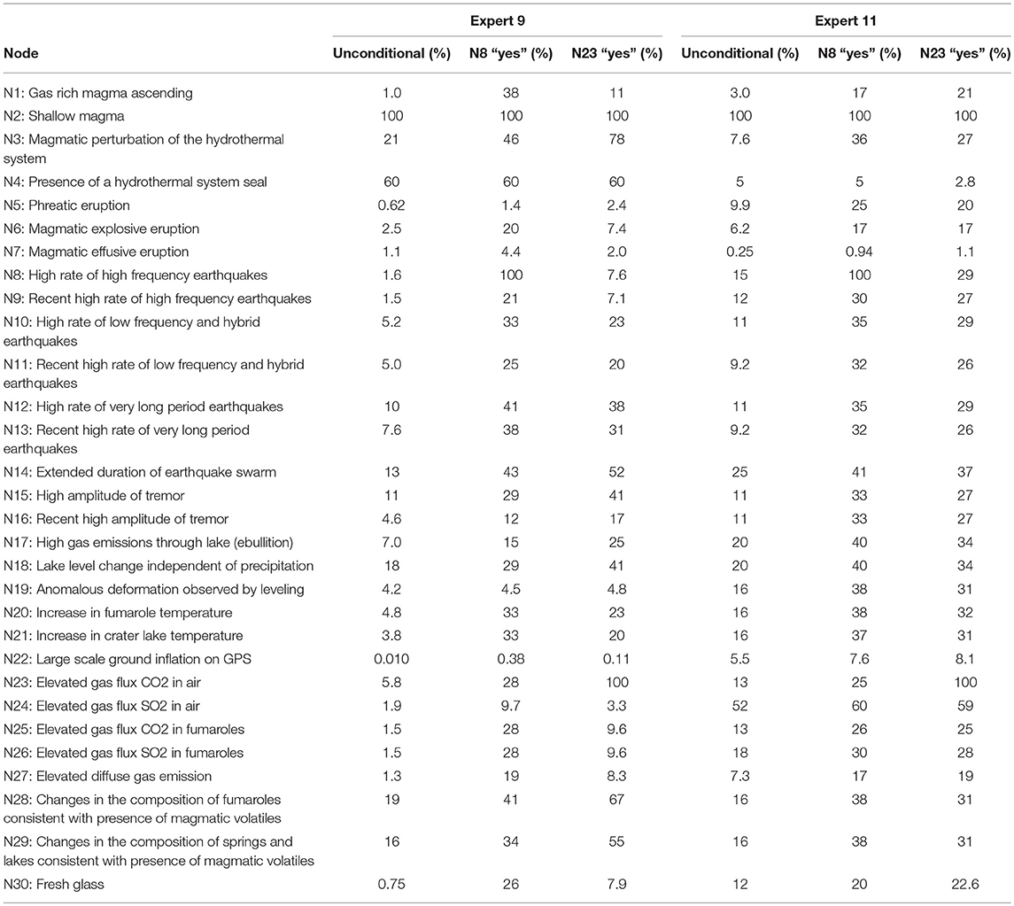
Table 3. The probability of “yes” for Expert 9 and 11 of observing each node for the unconditional Bayesian network with no evidence added, and evidence added to “yes” for node “N8: High rate of high frequency earthquakes” and node “N23: Elevated gas flux of CO₂ in air.”

Table 3 illustrates how adding evidence changes the probability of all nodes that are directly or indirectly connected, i.e., in our case nearly all nodes. For example, observing “High rate of high frequency earthquakes” makes “Elevated gas flux CO₂ in air” more likely (increase from 5.8 to 28% for Expert 9 and 13 to 25% for Expert 11) and observing “Elevated gas flux CO₂ in air” increases the probability for “high rate of high frequency earthquakes” from 1.6 to 7.6% for Expert 9 and from 15 to 29% for Expert 11. The influence of seeing one observable on the likelihood that another being positive can be explained by their indirect linkage via common unobservable volcanic process nodes (yellow nodes in Figure 5). In this instance, the CPTs of the observable nodes reflect judgments that these observables are more likely to occur when gas rich magma ascends (node 1), or when there is a magmatic perturbation of the hydrothermal system (node 3). Thus, using the equations outlined in Figure 2, the probabilities of nodes 1 and 3 both increase when one of the observables occurs. Higher probabilities for nodes 1 and 3 in turn increase the probabilities of the other observables. This bi-directionality is useful to explore the diagnostic sensitivity of the results (the eruption nodes 5–7) to observing individual nodes, as done in Table 4.

TABLE 4

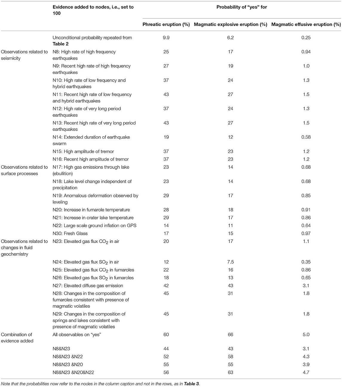
Table 4. For Expert 11, the probability of each of the three eruption types occurring in the next month (node = “yes”) given positive evidence is present for all observational nodes (in the rows), and the same eruption probabilities for different sub-combinations of observational nodes (at the bottom of the table).

An example of independent nodes is nodes 4 and 8. As a consequence of their independence, the probability of node 4 does not change when node 8 is instantiated. In contrast, there is a parent-child relationship between node 4 and node 23. For Expert 11, the probability of node 4 changes when node 23 is instantiated. However, this is not the case for Expert 9, who judged node 4 and node 23 to be independent by providing the same probabilities for the CPT of node 23 regardless of whether node 4 was “yes” or “no.”

Looking at the hidden nodes “N1: Gas rich magma ascending” and “N3: Magmatic perturbation of the hydrothermal system,” the effect of observing “N8: High rate of high frequency earthquakes” and “N23: Elevated gas flux CO₂ in air” is reversed for both experts: for Expert 9, the probability for node 1 increases from 1 to 38% for observing high frequency earthquakes, compared to only 11% for observing elevated CO₂ in air. This trend is reversed for node 3, where the probability increases from 21 to 46% for observing high frequency earthquakes but to 79% for elevated CO₂ in air. Expert 9's explanation for this is that a high rate of high frequency earthquakes is an indication of rock breaking, which is very likely caused by gas rich magma ascending. Other processes can also cause elevated CO₂ in air and there may also be a delay in CO₂ reaching air when gas rich magma is ascending. Other nodes that have a notable higher probability when conditioned on node 8, rather than on node 23 include “N7: Magmatic explosive eruption” and “N30: Fresh glass.” These outcomes are again consistent with fresh magma rising abruptly and breaking rocks along the way. Unfortunately, there was not time to discuss the results with all experts. Doing so, especially as a group process, can help to share, and perhaps resolve, differing understandings of the system.

A final example from Table 3 might initially appear counterintuitive: the probability of elevated gas flux CO₂ and SO₂ in fumaroles is higher for a high rate of high frequency earthquakes than for elevated CO₂ gas in air. This is the case for both Experts 9 and 11, but more so for Expert 9. Expert 9 estimates that node 1 has a much stronger influence on the gas flux in fumaroles than node 3. As discussed above, the probability of the former is much higher (38 vs. 11%) when a high rate of high frequency earthquakes is observed compared to elevated gas flux CO₂ in air.

Table 4 shows the probability of observing the different eruption types in the next month for Expert 11, given evidence for the individual observational nodes listed in the rows. For example, the largest increase in the probability of “yes” for “Magmatic explosive eruption” from an individual node comes from node “N28: Changes in the composition of fumaroles consistent with presence of magmatic volatiles” (45% compared to 9.9% for unconditional). This example illustrates how the BN method allows the probabilistic weights of different pieces of evidence to be enumerated, one against another, in a coherent and objective manner.

At the bottom of Table 4, we show the probability of the three eruption nodes for all observables happening at the same time, as well as different combinations of nodes. When all observables occur, the probabilities for eruption in the next month are 60% for “N5: Phreatic eruption,” 66% for “N6: Magmatic explosive eruption” and 5% for “N7: Magmatic effusive eruption.” In the following rows, we combine different nodes to explore which ones are most influential to get closest to the maximum probabilities found when all observables occur. The probabilities of eruption increase most for a combination of nodes from different areas of the BN, namely seismological and changes in fluid geochemistry.

Discussion and Recommendations

The aim of the pilot project was to explore the utility of BN modeling for eruption forecasting rather than to develop an operational model for short-term volcanic hazard assessment. The pilot provided opportunities for productive multi-disciplinary and international collaborations, and led to many useful insights that, most likely, would not have emerged without having a structured elicitation framework (detailed in the Supplementary Material).

The volcano monitoring team, as key stakeholder for assessing the usefulness of BN modeling for eruption forecasting, was involved in all stages of the pilot project. The team members participated enthusiastically and experts from New Zealand universities readily agreed to participate in the workshop to quantify the model. The strong engagement of volcanologists from within and outside the volcano monitoring team reflects the interest in probabilistic methods for eruption forecasting. The participants saw other possible applications of BNs in their own work, ranging from better understanding the volcano system to deciding what monitoring data were critical and where to put additional monitoring stations.

The development of the BN model structure provided a useful framework for experts from different sub-disciplines to share and synthesize their respective understandings of the volcano system. The graphical representation with simplified causal links proved to be an illuminating “prop” as different experts explained their interpretations of the various elements of the system. Thus, the BN concept enhanced scientific discussion between experts, who already regularly discuss Whakaari.

In the following, we highlight issues related to the model complexity, definitions of variables and states, and BN modeling in volcanology.

Clarity of Definitions for Nodes and States

Given the time constraints on the pilot study, we did not have the opportunity to discuss all nodes with all experts prior to the elicitation workshop. There was extensive discussion during the workshop although insufficient to gain clarity on all aspects. In particular, the node concerning the “Presence of the hydrothermal system seal” prompted debate among the experts. While written descriptions of each expert's understanding of the node are similar, the spread of probability judgments in questions involving this node indicates large uncertainty. Many experts commented that they were unsure how to deal with this node. This highlights that, while it is important for all experts to have as much clarity and agreement on all nodes in the BN as possible, such challenges are often intrinsic to a complex problem. Their emergence through elicitation and BN building often signal where critical and unresolved issues may exist. Any “hidden” nodes that describe the unobservable processes of the volcanic systems can be expected to be vaguer since experts inevitably have varying understandings of those processes.

For simplicity, the pilot model was configured with only two states for each variable. The experts did not agree that such a simplification was justified due to the continuous nature of data, which characterize most observables, and the wide range of values they can cover. Given the challenge to set thresholds to distinguish between the two states, we did not enforce consensus. Instead the experts provided their individual definition of thresholds when estimating the probabilities (see section Definitions of states). The different definitions of thresholds contributed to the spread in responses (Figure 6). Other eruption forecasting models have adopted fuzzy logic to deal with monitoring variables (e.g., Marzocchi et al., 2008; Selva et al., 2012). To distinguish a parameter “anomaly” from its “non-anomaly” state, two separate determinative thresholds are chosen, and a fuzzy function gauges the “degree of anomaly” in between. Within this approach, a probability density function is constructed for the event of interest, e.g., for (magmatic) unrest or eruption. Whilst, for simplicity, our workshop exercise adopted a basic two-state indicator for parameter conditions, for eruption forecasting we recommend working with a fully probabilistic approach that allows for modeling variables measured on a continuous scale with continuous probability density functions, instead of fuzzy logic. New modeling techniques make this feasible (Hanea et al., 2006; Cannavò et al., 2017).

Model Complexity

We included in the BN model all observables that are regularly monitored at Whakaari. The subsequent number of nodes in the pilot model created challenges for estimating the required probabilities and for further processing of the data. Within the 2 half-day workshop, our experts succeeded in estimating all required probabilities, as well as provide comments on other aspects of the model and the elicitation process. However, informal feedback indicates that it would have been better to have longer to think about individual variables. This feedback is reflected in the spread of responses to some questions (see Figure 6).

Experts commented in the feedback questionnaire that there were too many nodes for observations related to seismicity and to changes in fluid geochemistry. In particular, the nodes related to recent seismicity did not “behave” as expected. Table 4 indicates that the different seismicity nodes and the different fluid geochemistry nodes have the same effect on the query nodes of eruption. Thus, there could be fewer nodes without loss of information.

For eruption forecasting, the main factor governing the number of BN nodes is the number of variables being monitored and observed. Under crisis conditions, these might comprise four or more data streams; typical examples are: transient or tremor seismicity, such as conduit-related or spatially diffuse VTs and LF/hybrid seismicity; geodetic cGPS deformation for deep pressurization, or EDM distance measurements, tiltmeters, or radar techniques for shallow/surface movements; gas fluxes, from DOAS, COSPEC; thermal and remote sensing images; geophysical measurements such as gravity, resistivity; and hydrological measurements (see e.g., Science Advisory Committee for the assessment of the hazards risks associated with the Soufrière Hills Volcano Montserrat, 2005; Aspinall and Woo, 2014). If, however, the BN needs to reflect time-varying states, the number of nodes overall can easily exceed 12 or more (e.g., Hincks et al., 2014); in this regard, much depends on how close the volcanic system behavior is to stationary. With modern computers, the processing burden for a large BN is not critical and, when data are plentiful, it is feasible to test how much information each node contributes: it generally makes sense to omit nodes (or links) which do not add much information to the outcome or decision. For example, the UNINET BN program (available at: http://www.lighttwist.net/wp/) can automatically eliminate links if an individual conditional correlation is below some threshold. Similarly, tests of a BN for lahar probability on Montserrat, which re-learned its correlations at each time step starting from time zero, stabilized after about 10 lahar events had been observed (T. Hincks, pers. comm.).

The other key factor, which unquestionably will influence the tractability of a complex BN in a crisis application, is whether there is a person available with the time and knowledge to run the BN and communicate the results. In principle, a volcano observatory should have someone who continually monitors hazard and risk levels, just as colleagues monitor physical variables such as seismicity and fluid geochemistry in real time.

BN Modeling in Volcano Monitoring

Our pilot project and several recent publications of BN applications in volcano monitoring and volcanic multi-hazard assessment (Aspinall and Woo, 2014; Cannavò et al., 2017; Sheldrake et al., 2017; Tierz et al., 2017) clearly demonstrate the usefulness of BN modeling for different aspects of volcano monitoring, including eruption forecasting. We briefly focus below on three areas that are important for future BN model development for eruption forecasting: continuous variables, dynamic system and expert involvement.

Continuous Variables

One of the main challenges in the model development of the pilot study was defining thresholds for the states of each node, because the experts had reservations about representing continuous observable data with just two states in the BN model. The answer to this challenge is working with continuous variables to reflect the nature of most monitoring data. However, there is less software available for this task, and more importantly most modeling techniques for continuous variables assume joint normality of the data. The assumption of joint normality seems valid on Mount Etna, Italy (Cannavò et al., 2017), where the volcanic activity appears much more regular than most volcanoes around the world. However, the upper tails of many volcanological datasets exhibit dependencies upon each other. For example, while observing an extreme value of any one particular variable is unlikely, if one variable, such as seismicity, is very high, it is more likely that another, e.g., gas flux, is also high. Thus, the assumption of joint normal properties cannot properly represent tail dependence (e.g., Joe, 2014). One possible solution is to condition the BN on a period of unrest and only consider the distribution of variables for that time period.

We have started to work on a BN model to answer the question whether a period of unrest will lead to a large eruption for New Zealand volcanoes. We recommend investing time and effort into developing BN modeling techniques for eruption forecasting to expand the availability of tools for future hazard and risk assessments.

Dynamic System

Volcanoes are dynamic systems with magma undergoing profound changes in physical properties during ascent prior to an eruption (Sparks, 2003). As a consequence, the relationship between system variables may change considerably over time. Dynamic BNs can model sequences of events with changing dependencies. Basic applications in volcanology include Aspinall et al. (2006) and a simplified time-stepping BN used by Aspinall and Woo (2014), while Hincks et al. (2014) outline the potential for developing models that include temporal relationships between nodes of a volcanological dynamic BN. We recommend further exploring the use of dynamic BNs to get a better understanding of the volcanic processes.

Stakeholder and Expert Involvement

Volcano experts assess crisis situations and advise on what might happen next. We do not intend for BNs or any other quantitative tools to replace the role of a volcano monitoring team. However, quantitative decision-support tools are crucial to provide a reproducible, transparent, and documented framework for giving advice during a crisis.

It is important for the experts who use quantitative models to understand model limitations. Therefore, we recommend that the wider volcano monitoring team is involved in the model development and that a BN model owner, who orchestrates the development of and maintains the model when it is complete (or hands it over to another to run for repeated analyses), is identified.

In the future, we recommend engaging with stakeholders beyond the volcano monitoring team during all stages of the model development for wider model buy-in.

Despite efforts to build a library of worldwide volcanic unrest data (Newhall et al., 2017), future BN model developments for volcano hazard and risk assessments are likely to involve expert judgment due to limited data on most volcanoes, even in well-monitored volcanic centers, such as those in New Zealand. We recommend following structured expert elicitation procedures (e.g., Hanea et al., 2016). We also recommend weighting experts according to their ability to quantify topic-specific uncertainties based on seed items with known values (e.g., Colson and Cooke, 2017). In the pilot study we did not use weighting because we did not have the resources to develop calibration questions appropriate for target questions on conditional probabilities. It will be easier to develop appropriate calibration questions for continuous BNs when asking for uncertainties associated with physical data, rather than with probabilities.

We strongly encourage discussion among experts to share their knowledge and understanding of the volcanic system in an environment conducive for open discussion yet. At the same time, the elicitation procedure should allow experts to express their own scientific beliefs without peer-group or institutional pressures.

When developing a model for a volcano monitoring team, we recommend the inclusion of external experts for an outside perspective. This additional logistical effort and requirement of resources will have to be balanced carefully with the purpose of the model.

For the development of the model structure, it would be useful to select an interested available representative of each sub-discipline. The representative experts can then explain their rationale about the chosen variables and their relationships. Unfortunately, there is little existing guidance on qualitative expert elicitation, such as the development of the model structure. Research into procedures for this is warranted.

Conclusions

We have started exploring the potential of BN modeling for eruption forecasting in New Zealand. While our pilot study of a discrete model to forecast eruptions on Whakaari did not yield a tool ready for application, it provided substantial benefits to the science team involved. In particular, the development of the model structure allowed experts from different sub-disciplines to share their respective understanding of the mechanisms and processes leading to eruption. The simplified graphical presentation of the volcanic system highlighted assumptions that were made by individual sub-disciplines but not necessarily widely appreciated before.

We have found that BNs offer a flexible framework to address many questions in volcano monitoring and volcanic hazard and risk assessment. We anticipate that the BN approach will become essential for handling ever-burgeoning observations and amounts of monitoring data, and indispensable for assessing their evidential meaning for operational eruption forecasting. Further research into these techniques, in particular continuous and dynamic modeling, will extend the scope for useful applications.

Our four key recommendations for future work are: (1) building causal BN sub-models that allow experts from different sub-disciplines to express their knowledge and understanding of particular volcanic processes, which can then be combined into an over-arching volcanic system network; (2) applying BN modeling techniques for continuous variables that more naturally reflect volcano-monitoring data; (3) carefully choosing the number of variables to be modeled; and (4) using robust methods, including structured expert judgment.

Moreover, it is vital that time and effort is invested in developing any BN forecast decision support tool well before the next volcanic crisis starts. Once unrest data is coming in, attention should be given to updating the quantitative aspects of the network with the data observed.

Ethics Statement

This study was carried out in accordance with the recommendations of Code of Ethical Conduct, Massey University, New Zealand. The study was evaluated to be of low-risk of harm to the participants. Consequently a Low Risk Notification was submitted to Massey University. All participants gave written informed consent.

Author Contributions

AC initiated and led the pilot project. AC, ND, and LC were part of the initial team that adapted the structure of La Soufrière volcano, Guadeloupe, to Whakaari, New Zealand and drafted the first questionnaire to elicit the conditional probability tables. NF was the official project owner; he also helped revise the model structure and advised on the experts to include in the elicitation. AC organized and facilitated the expert elicitation workshop, where ND, LC, and NF were three of the 11 participating experts, and ND facilitated an exercise on calibration questions. AC processed the results, compiled the report of preliminary results, and led the writing of the manuscript. WA provided guidance and support throughout the study. AH reviewed the preliminary results and guided the development of an initial continuous BN for New Zealand, with LC and NF being the key contributors. All authors contributed to writing of the manuscript.

Funding

The pilot project was supported by GNS Science Strategic Science Research funding and by GNS Science Core Research Programme funding.

Conflict of Interest Statement

The authors declare that the research was conducted in the absence of any commercial or financial relationships that could be construed as a potential conflict of interest.

Acknowledgments

We thank Gill Jolly for setting up the initial team and getting the pilot project started. Rob Buxton and Sally Potter were part of the initial team and we thank Sally for overseeing the ethics application process. Katy Kelly and Kat Hammond helped with setting up the questionnaires and administrative support for workshop organization and report formatting. Art Jolly, Steve Sherburn, Bruce Christenson, and Tony Hurst revised the initial model structure and Tony helped describing all variables for workshop notes. We thank our 11 experts at the elicitation workshop for their essential and constructive contibutions: LC, ND, NF, Tony Hurst, Art Jolly, Geoff Kilgour, Jan Lindsay, Agnes Mazot, Jon Procter, Brad Scott and Steve Sherburn. Without the support and enthusiasm of the volcano monitoring team to explore BN modeling the study would not have been possible. We thank Brad Scott for providing information on Whakaari for completing the manuscript. We are grateful to David Rhoades and Ken Gledhill, who reviewed the manuscript before submission. We thank an anonymous reviewer, Stephen McNutt, Pablo Tierz and the associate editor John Stix for their valuable comments, which improved the manuscript.

Supplementary Material

The Supplementary Material for this article can be found online at: https://www.frontiersin.org/articles/10.3389/feart.2018.00211/full#supplementary-material Supplementary material provides more detail on “Quantifying the pilot model” and includes the workshop notes and the questionnaires.

References

Aspinall, W. P. (2006). “Structured elicitation of expert judgement for probabilistic hazard and risk assessment in volcanic eruptions,” in Statistics in Volcanology, eds H. M. Mader, S. G. Coles, C. B. Connor, and L. J. Connor (London: Geological Society), 15–30.

Google Scholar

Aspinall, W. P. (2010). A route to more tractable expert advice. Nature 463, 294–295. doi: 10.1038/463294a

PubMed Abstract | CrossRef Full Text | Google Scholar

Aspinall, W. P., Carniel, R., Jaquet, O., Woo, G., and Hincks, T. (2006). Using hidden multi-state Markov models with multi-parameter volcanic data to provide empirical evidence for alert level decision-support. J. Volcanol. Geothermal Res. 153, 112–124. doi: 10.1016/j.jvolgeores.2005.08.010

CrossRef Full Text | Google Scholar

Aspinall, W. P., and Woo, G. (2014). Santorini unrest 2011–2012: an immediate Bayesian belief network analysis of eruption scenario probabilities for urgent decision support under uncertainty. J. Appl. Volcanol. 3, 1–12. doi: 10.1186/s13617-014-0012-8

CrossRef Full Text | Google Scholar

Aspinall, W. P., Woo, G., Voight, B., and Baxter, P. J. (2003). Evidence-based volcanology: application to eruption crises. J. Volcanol. Geothermal Res. 128, 273–285. doi: 10.1016/S0377-0273(03)00260-9

CrossRef Full Text | Google Scholar

Barclay, J., Haynes, K., Houghton, B., and Johnston, D. (2015). “Chapter 69 - social processes and volcanic risk reduction A2 - Sigurdsson, Haraldur,” in The Encyclopedia of Volcanoes, 2nd Edn, eds H. Sigurdsson, B. Houghton, S. McNutt, H. Rymer, and J. Stix (Amsterdam: Academic Press), 1203–1214. doi: 10.1016/B978-0-12-385938-9.00069-9

CrossRef Full Text | Google Scholar

Bayes, M., and Price, M. (1763). An essay towards solving a problem in the doctrine of chances. By the Late Rev. Mr. Bayes, F. R. S. communicated by Mr. Price, in a Letter to John Canton, A. M. and F. R. S. Philos. Trans. 53, 370–418. doi: 10.1098/rstl.1763.0053

CrossRef Full Text | Google Scholar

Bebbington, M. S., Stirling, M. W., Cronin, S., Wang, T., and Jolly, G. (2018). National-level long-term eruption forecasts by expert elicitation. Bull. Volcanol. 80:56. doi: 10.1007/s00445-018-1230-4

CrossRef Full Text | Google Scholar

Black, P. M. (1970). Observations on white island volcano, New Zealand. Bull. Volcanol. 34, 158–167. doi: 10.1007/BF02597783

CrossRef Full Text | Google Scholar

Burgman, M. A., McBride, M., Ashton, R., Speirs-Bridge, A., Flander, L., Wintle, B., et al. (2011). Expert status and performance. PLoS ONE 6:e22998. doi: 10.1371/journal.pone.0022998

PubMed Abstract | CrossRef Full Text | Google Scholar

Burns, Z., Chiu, A., and Wu, G. et al. (2010). “Overweighting of Small Probabilities,” in Wiley Encyclopedia of Operations Research and Management Science, ed J. J. Cochran (Hoboken, NJ: John Wiley & Sons, Inc.), 1–8. doi: 10.1002/9780470400531.eorms0634

CrossRef Full Text | Google Scholar

Cannavò, F., Cannata, A., Cassisi, C., Di Grazia, G., Montalto, P., Prestifilippo, M., et al. (2017). A multivariate probabilistic graphical model for real-time volcano monitoring on Mount Etna. J. Geophys. Res. 122, 3480–3496. doi: 10.1002/2016JB013512

CrossRef Full Text | Google Scholar

Chardot, L., Jolly, A. D., Kennedy, B. M., Fournier, N., and Sherburn, S. (2015). Using volcanic tremor for eruption forecasting at White Island volcano (Whakaari), New Zealand. J. Volcano Geothermal Res. 302, 11–23. doi: 10.1016/j.jvolgeores.2015.06.001

CrossRef Full Text | Google Scholar

Christenson, B. W., White, S., Britten, K., and Scott, B. J. (2017). Hydrological evolution and chemical structure of a hyper-acidic spring-lake system on Whakaari/White Island, NZ. J. Volcanol. Geothermal Res. 346, 180–211. doi: 10.1016/j.jvolgeores.2017.06.017

CrossRef Full Text | Google Scholar

Christophersen, A. (2017). Forecasting Volcanic Eruptions on White Island in the Next Month With Bayesian Network Modelling: Preliminary Results From an Expert Elicitation Workshop. Lower Hutt: GNS Science.

Christophersen, A., Rhoades, D. A., Gerstenberger, M. C., Bannister, S., Becker, J., Potter, S. H., et al. (2017). “Progress and challenges in operational earthquake forecasting in New Zealand,” in New Zealand Society for Earthquake Engineering Technical Conference (Wellington: New Zealand Society for Earthquake Engineering).

Google Scholar

Clark, R. H., and Otway, P. M. (1989). Deformation monitoring associated with the 1976-82 White Island eruption sequence. N. Z. Geol. Survey Bull. 103, 69–84.

Clemen, R. T., and Winkler, R. L. (1999). Combining probability distributions from experts in risk analysis. Risk Anal. 19, 187–203. doi: 10.1111/j.1539-6924.1999.tb00399.x

CrossRef Full Text | Google Scholar

Cole, J. W., and Lewis, K. B. (1981). Evolution of the Taupo-Hikurangi subduction system. Tectonophysics 72, 1–21. doi: 10.1016/0040-1951(81)90084-6

CrossRef Full Text | Google Scholar

Cole, J. W., and Nairn, I. A. (1975). Catalogue of the Active Volcanoes of the World Including Solfatara Fields. Part 22: New Zealand. Naples: International Association of Volcanology and Chemistry of the Earth's Interior.

Cole, J. W., Thordarson, T., and Burt, R. (2000). Magma origin and evolution of White Island (Whakaari) Volcano, Bay of Plenty, New Zealand. J. Petrol. 41, 867–895. doi: 10.1093/petrology/41.6.867

CrossRef Full Text | Google Scholar

Colson, A. R., and Cooke, R. M. (2017). Cross validation for the classical model of structured expert judgment. Reliabil. Eng. Syst. Safety 163, 109–120. doi: 10.1016/j.ress.2017.02.003

CrossRef Full Text | Google Scholar

Cooke, R. M. (1991). Experts in Uncertainty: Opinion and Subjective Probability in Science. Oxford University Press.

Cooke, R. M., and Goossens, L. L. H. J. (2008). TU Delft expert judgment data base. Reliab. Eng. Syst. Saf. 93, 657–674. doi: 10.1016/j.ress.2007.03.005

CrossRef Full Text | Google Scholar

Deligne, N. I., Jolly, G. E., Taig, T., and Webb, T. H. (2018). Evaluating life-safety risk for fieldwork on active volcanoes: the volcano life risk estimator (VoLREst), a volcano observatory's decision-support tool. J. Appl. Volcanol. 7:7. doi: 10.1186/s13617-018-0076-y

CrossRef Full Text | Google Scholar

Fenton, N., and Neil, M. (2013). Risk Assessment and Decision Analysis with Bayesian Networks. Boca Raton, FL: CRC Press.

Google Scholar

Fournier, N., and Chardot, L. (2012). Understanding volcano hydrothermal unrest from geodetic observations: Insights from numerical modeling and application to White Island volcano, New Zealand. J. Geophys. Res. 117:B11208. doi: 10.1029/2012JB009469

CrossRef Full Text | Google Scholar

GeoNet (2018). Volcanic Alert Bulletins. Available online at: http://www.geonet.org.nz/volcano/vab (Accessed February 07, 2018).

Gerstenberger, M. C., and Christophersen, A. (2016). A bayesian network and structured expert elicitation for Otway stage 2C: detection of injected CO2 in a saline aquifer. Int. J. Greenhouse Gas Contr. 51, 317–329. doi: 10.1016/j.ijggc.2016.05.011

CrossRef Full Text | Google Scholar

Gerstenberger, M. C., Christophersen, A., Buxton, R., and Nicol, A. (2015). Bi-directional risk assessment in carbon capture and storage with Bayesian Networks. Int. J. Greenhouse Gas Contr. 35, 150–159. doi: 10.1016/j.ijggc.2015.01.010

CrossRef Full Text | Google Scholar

Gerstenberger, M. C., and Rhoades, D. A. (2010). New Zealand earthquake forecast testing centre. Pure Geophys. 167, 877–892. doi: 10.1007/s00024-010-0082-4

CrossRef Full Text | Google Scholar

Giggenbach, W. F., and Glasby, G. P. (1977). The influence of thermal activity on the trace metal distribution in marine sediments around White Island, New Zealand. DSIR Res. Bull. 218, 121–126.

Giggenbach, W. F., and Sheppard, D. S. (1989). Variations in the temperature and chemistry of White Island fumarole discharges 1972-85. N. Z. Geol. Survey Bull. 103, 119–126.

Hanea, A. M., Kurowicka, D., and Cooke, R. M. (2006). Hybrid method for quantifying and analyzing bayesian belief nets. Qual. Reliabil. Eng. Int. 22, 709–729. doi: 10.1002/qre.808

CrossRef Full Text | Google Scholar

Hanea, A. M., McBride, M. F., Burgman, M. A., and Wintle, B. C. (2016). Classical meets modern in the IDEA protocol for structured expert judgement. J. Risk Res. 21, 417–433. doi: 10.1080/13669877.2016.1215346

CrossRef Full Text | Google Scholar

Hincks, T. K., Komorowski, J. C., Sparks, S. R., and Aspinall, W. P. (2014). Retrospective analysis of uncertain eruption precursors at La Soufrière volcano, Guadeloupe, 1975–77: volcanic hazard assessment using a Bayesian Belief Network approach. J. Appl. Volcanol. 3, 1–26. doi: 10.1186/2191-5040-3-3

CrossRef Full Text | Google Scholar

Højsgaard, S. (2012). Graphical independence networks with the gRain package for R. J. Stat. Softw. 46, 1–26. doi: 10.18637/jss.v046.i10

CrossRef Full Text | Google Scholar

Houghton, B. F., and Nairn, I. A. (1989). A model for the 1976-82 phreatomagmatic and strombolian eruption sequence at White Island volcano, New Zealand. N. Z. Geol. Survey Bull. 103, 127–137.

Google Scholar

Houghton, B. F., and Nairn, I. A. (1991). The 1976-82 strombolian and phreatomagmatic eruptions of White Island, New Zealand: eruptive and depositional mechanisms at a “wet” volcano. Bull. Volcanol. 54, 25–49.

Google Scholar

Hurst, A. W., Rickerby, P., Scott, B. J., and Hashimoto, T. (2004). Magnetic field changes on White Island, New Zealand, and the value of magnetic changes for eruption forecasting. J. Volcanol. Geotherm. Res. 54, 25–49. doi: 10.1016/j.jvolgeores.2004.03.017

CrossRef Full Text | Google Scholar

Ingham, M. R. (1992). Audiomagnetotelluric soundings on White Island volcano. J. Volcanol. Geotherm. Res. 50, 301–306. doi: 10.1016/0377-0273(92)90098-X

CrossRef Full Text | Google Scholar

Joe, H. (2014). Dependence Modeling With Copulas. Boca Raton, FL: CRC Press.

Google Scholar

Jolly, G. E., Keys, H. J. R., Procter, J. N., and Deligne, N. I. (2014). Overview of the co-ordinated risk-based approach to science and management response and recovery for the 2012 eruptions of Tongariro volcano, New Zealand. J. Volcanol. Geotherm. Res. 286, 184–207. doi: 10.1016/j.jvolgeores.2014.08.028

CrossRef Full Text | Google Scholar

Kato, A., Terakawa, T., Yamanaka, Y., Maeda, Y., Horikawa, S., Matsuhiro, K., et al. (2015). Preparatory and precursory processes leading up to the 2014 phreatic eruption of Mount Ontake, Japan. Earth Planets Space 67:111. doi: 10.1186/s40623-015-0288-x

CrossRef Full Text | Google Scholar

Kilgour, G., Moune, S., Della Pasqua, F., and Christenson, B. (2016). Petrological Insights into the 1976-2000 Eruption Episode of White Island, New Zealand: An Eruption Fuelled by Repeated Mafic Recharge. Vienna.

Google Scholar

Koller, D., and Friedman, N. (2009). Probabilistic Graphical Models: Principles and Techniques. Cambridge, MA: MIT Press Ltd.

Google Scholar

Konstantinou, K. I., and Schlindwein, V. (2003). Nature, wavefield properties and source mechanism of volcanic tremor: a review. J. Volcanol. Geotherm. Res. 119, 161–187. doi: 10.1016/S0377-0273(02)00311-6

CrossRef Full Text | Google Scholar

Korb, K. B., and Nicholson, A. E. (2010). Bayesian Artificial Intelligence, 2nd Edn. Boca Raton, FL: CRC Press, Inc.

Google Scholar

Langseth, H., Nielsen, T. D., Rum,í, R., and Salmerón, A. (2009). Inference in hybrid Bayesian networks. Reliabil. Eng. Syst. Saf. 94, 1499–1509. doi: 10.1016/j.ress.2009.02.027

CrossRef Full Text | Google Scholar

Latter, J. H., Scott, B. J., and Dibble, R. (1989). Seismic activity associated with the 1976-82 eruption sequence at White Island volcano. N. Z. Geol. Survey Bull. 103, 85–107.

Google Scholar

Lindsay, J., Marzocchi, W., Jolly, G., Constantinescu, R., Selva, J., and Sandri, L. (2010). Towards real-time eruption forecasting in the Auckland Volcanic Field: application of BET_EF during the New Zealand National Disaster Exercise ‘Ruaumoko'. Bull. Volcanol. 72, 185–204. doi: 10.1007/s00445-009-0311-9

CrossRef Full Text | Google Scholar

Martí, J., Aspinall, W. P., Sobradelo, R., Felpeto, A., Geyer, A., Ortiz, R., et al. (2008). A long-term volcanic hazard event tree for Teide-Pico Viejo stratovolcanoes (Tenerife, Canary Islands). J. Volcanol. Geotherm. Res. 178, 543–552. doi: 10.1016/j.jvolgeores.2008.09.023

CrossRef Full Text | Google Scholar

Marzocchi, W., Sandri, L., and Selva, J. (2008). BET_EF: a probabilistic tool for long- and short-term eruption forecasting. Bull. Volcanol. 70, 623–632. doi: 10.1007/s00445-007-0157-y

CrossRef Full Text | Google Scholar

McNutt, S. R. (2005). Volcanic seismology. Ann. Rev. Earth Planet. Sci. 32, 461–491. doi: 10.1146/annurev.earth.33.092203.122459

CrossRef Full Text | Google Scholar

Murphy, K. P. (2012). Machine Learning: A Probabilistic Perspective. Cambridge, MA: The MIT Press.

Neri, A., Aspinall, W. P., Cioni, R., Bertagnini, A., Baxter, P. J., Zuccaro, G., et al. (2008). Developing an event tree for probabilistic hazard and risk assessment at Vesuvius. J. Volcanol. Geotherm. Res. 178, 397–415. doi: 10.1016/j.jvolgeores.2008.05.014

CrossRef Full Text | Google Scholar

New Zealand Ministry of Civil Defence and Emergency Management (2015). “Volcanic unrest or eruption,” in The Guide to the National Civil Defence Emergency Management Plan 2015 (Wellington: New Zealand Department of the Prime Minister and Cabinet).

Newhall, C. G., Costa, F., Ratdomopurbo, A., Venezky, D. Y., Widiwijayanti, C., Win, N. T. Z., et al. (2017). WOVOdat – An online, growing library of worldwide volcanic unrest. J. Volcanol. Geotherm. Res. 345, 184–199. doi: 10.1016/j.jvolgeores.2017.08.003

CrossRef Full Text | Google Scholar

Newhall, C. G., and Hoblitt, R. (2002). Constructing event trees for volcanic crises. Bull. Volcanol. 64, 3–20. doi: 10.1007/s004450100173

CrossRef Full Text | Google Scholar

Nishi, Y., Ishido, T., Matsumoto, N., Ogawa, Y., Tosha, T., Miyazaki, J., et al. (1996a). “Self-potential and audio-magnetotelluric survey in White Island Volcano,” in Proceedings 18th NZ Geothermal Workshop. (Auckland: University of Auckland), 237–242.

Google Scholar

Nishi, Y., Sherburn, S., Scott, B. J., and Sugihara, M. (1996b). High-frequency earthquakes at White Island volcano, New Zealand: insights into the shallow structure of a volcano-hydrothermal system. J. Volcanol. Geotherm. Res. 72, 183–197. doi: 10.1016/0377-0273(96)00005-4

CrossRef Full Text | Google Scholar

Norsys (1995-2018). Netica Application. Available online at: https://norsys.com/netica.html (Accessed August 10, 2018).

O'Hagan, A., Buck, C. E., Daneshkhah, A., Eiser, J. R., Garthwaite, P. H., Jenkinson, D. J., et al. (2006). Uncertain Judgements: Eliciting Experts' Probabilities. London: Wiley.

Google Scholar

Pearl, J. (1988). Probabilistic Reasoning in Intelligent Systems: Networks of Plausible Inference. San Francisco, CA: Morgan Kaufmann Publishers.

Google Scholar

Pearl, J., and Russel, S. (2001). “Bayesian networks. Report (R-277), November 2000,” in Handbook of Brain Theory and Neural Networks, ed M. Arbib (Cambridge: MIT Press), 157–160.

Peltier, A., Scott, B. J., and Hurst, T. (2009). Ground deformation patterns at White Island volcano (New Zealand) between 1967 and 2008 deduced from levelling data. J. Volcanol. Geotherm. Res. 181, 207–218. doi: 10.1016/j.jvolgeores.2009.01.020

CrossRef Full Text | Google Scholar

Potter, S. H., Jolly, G. E., Neall, V. E., Johnston, D. M., and Scott, B. J. (2014). Communicating the status of volcanic activity: revising New Zealand's volcanic alert level system. J. Appl. Volcanol. 3:13. doi: 10.1186/s13617-014-0013-7

CrossRef Full Text | Google Scholar

Pourret, O., Naïm, P., and Marcot, B. (2008). Bayesian Networks: A Practical Guide to Applications. Chichester, West Sussex, UK: Wiley.

Google Scholar

Rhoades, D. A., Liukis, M., Christophersen, A., and Gerstenberger, M. C. (2016). Retrospective tests of hybrid operational earthquake forecasting models for Canterbury. Geophys. J. Int. 204, 440–456. doi: 10.1093/gji/ggv447

CrossRef Full Text | Google Scholar

Science Advisory Committee for the assessment of the hazards and risks associated with the Soufrière Hills Volcano Montserrat (2005). Fourth Report of the Scientific Advisory Committee on Montserrat Volcanic Activity. Part II: Technical Report.

Selva, J., Marzocchi, W., Papale, P., and Sandri, L. (2012). Operational eruption forecasting at high-risk volcanoes: the case of Campi Flegrei, Naples. J. Appl. Volcanol. 1:5. doi: 10.1186/2191-5040-1-5

CrossRef Full Text | Google Scholar

Shachter, R. D., and Kenley, C. R. (1989). Gaussian influence diagrams. Manage. Sci. 35, 527–550. doi: 10.1287/mnsc.35.5.527

CrossRef Full Text | Google Scholar

Sheldrake, T. E., Aspinall, W. P., Odbert, H. M., Wadge, G., and Sparks, R. S. J. (2017). Understanding causality and uncertainty in volcanic observations: An example of forecasting eruptive activity on Soufrière Hills Volcano, Montserrat. J. Volcanol. Geotherm. Res. 341, 287–300. doi: 10.1016/j.jvolgeores.2017.06.007

CrossRef Full Text | Google Scholar

Sherburn, S., Scott, B. J., Nishi, Y., and Sugihara, M. (1998). Seismicity at White Island volcano, New Zealand: a revised classification and inferences about source mechanism. J. Volcanol. Geotherm. Res. 83, 287–312. doi: 10.1016/S0377-0273(98)00022-5

CrossRef Full Text | Google Scholar

Sparks, R. S. J. (2003). Forecasting volcanic eruptions. Earth Planet. Sci. Lett. 210, 1–15. doi: 10.1016/S0012-821X(03)00124-9

CrossRef Full Text | Google Scholar

Sparks, R. S. J., Biggs, J., and Neuberg, J. W. (2012). Monitoring volcanoes. Science 335:1310. doi: 10.1126/science.1219485

PubMed Abstract | CrossRef Full Text | Google Scholar

Spirtes, P., Glymour, C., and Scheines, R. (1993). Causation, Prediction, and Search. New York, NY: Springer Verlag.

Google Scholar

Tierz, P., Sandri, L., Costa, A., Sulpizio, R., Zaccarelli, L., Di Vito, M. A., et al. (2016a). “Uncertainty assessment of pyroclastic density currents at mount vesuvius (Italy) simulated through the energy cone model,” in Natural Hazard Uncertainty Assessment: Modeling and Decision Support, eds K. Riley, P. Webley and M. Thompson (Hoboken, NJ: Wiley; Washington, DC: American Geophysical Union), 125–145.

Google Scholar

Tierz, P., Sandri, L., Costa, A., Zaccarelli, L., Di Vito, M. A., Sulpizio, R., et al. (2016b). Suitability of energy cone for probabilistic volcanic hazard assessment: validation tests at Somma-Vesuvius and Campi Flegrei (Italy). Bull. Volcanol. 78:79. doi: 10.1007/s00445-016-1073-9

CrossRef Full Text | Google Scholar

Tierz, P., Woodhouse, M. J., Phillips, J. C., Sandri, L., Selva, J., Marzocchi, W., et al. (2017). A Framework for probabilistic multi-hazard assessment of rain-triggered lahars using Bayesian belief networks. Front. Earth Sci. 5:73. doi: 10.3389/feart.2017.00073

CrossRef Full Text | Google Scholar

Wadge, G., and Aspinall, W. P. (2014). Chapter 24 a review of volcanic hazard and risk-assessment praxis at the Soufrière Hills Volcano, Montserrat from 1997 to 2011. Geol. Soc. Lond. Memoirs 39, 439–456. doi: 10.1144/M39.24

CrossRef Full Text | Google Scholar

Weber, P., Medina-Oliva, G., Simon, C., and Iung, B. (2012). Overview on Bayesian networks applications for dependability, risk analysis and maintenance areas. Eng. Appl. Artif. Intell. 25, 671–682. doi: 10.1016/j.engappai.2010.06.002

CrossRef Full Text | Google Scholar

Werner, C., Hurst, T., Scott, B., Sherburn, S., Christenson, B. W., Britten, K., et al. (2008). Variability of passive gas emissions, seismicity, and deformation during crater lake growth at White Island Volcano, New Zealand, 2002–2006. J. Geophys. Res. 113:B01204. doi: 10.1029/2007JB005094

CrossRef Full Text | Google Scholar