Lagrangian Detection of Moisture Sources for the Southern Patagonia Icefield (1979–2017)

1. Introduction

The Southern Patagonia Icefield is the biggest temperate ice mass in the Southern Hemisphere, and thus an important fresh water storage for southern South America. It is located at the southern end of the Andes cordillera between 48.3 and 51.0°S along 73.0°W with an average width of 30–40 km and the narrowest section being 8 km wide (Figure 1) (Aniya et al., 1996). The icefield consists of 48 major outlet glaciers and over 100 small cirque and valley glaciers and has an average elevation of 1,600 m above mean sea level (m msl), while the icefield extends from the sea level with the highest peaks reaching above 3.000 m msl. Overall the climate can be summarized as temperate, very humid with freezing levels generally above 1 km msl, with a modest annual cycle and high annual precipitation rates (Miller, 1976; Weischet, 1996; Garreaud et al., 2013). Extreme environmental conditions and inaccessibility of the icefield pose a challenge for scientists to acquire records of meteorological conditions.

FIGURE 1

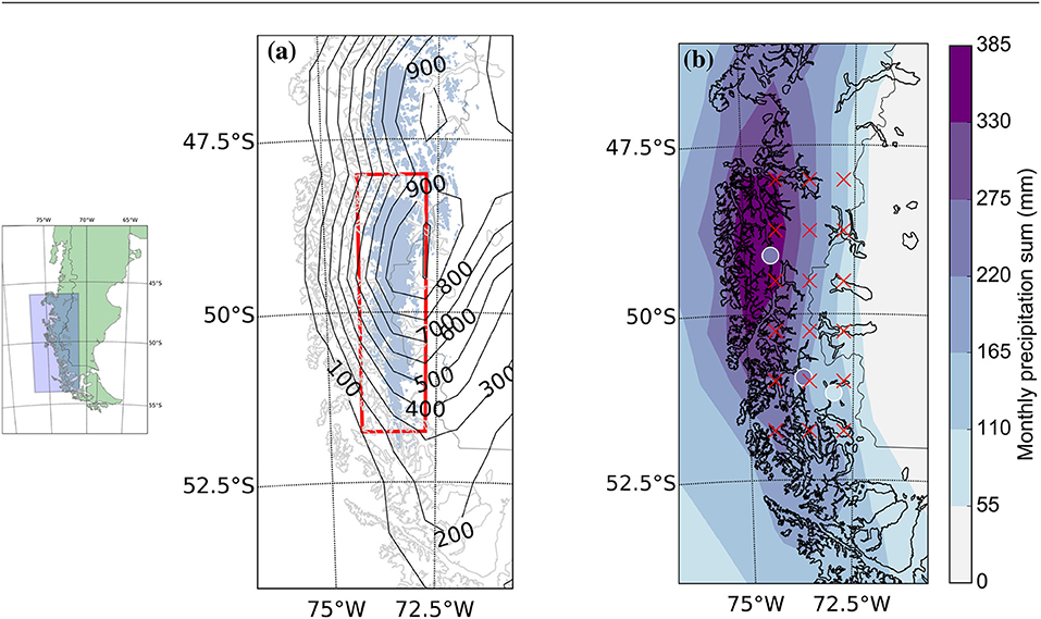
Figure 1. (a) ERA-Interim model topography in meters (contour lines) and the Patagonian icefields (light blue). The red rectangle illustrates the target area. (b) ERA-Interim total monthly mean precipitation and raw measurements of automatic weather stations from north to south: Puerto Eden, Amalia, Torres del Paine. The red crosses illustrate the trajectory starting positions.

The reconstruction of past climate behavior is essential to predict accurate the development of the icefield. Appropriate climate proxies are the stable isotopes of hydrogen and oxygen contained in firn and ice cores, adjacent lakes (sediments), and nearby vegetation. The isotope composition is mainly dependent on the moisture source, the sea surface temperature of marine moisture sources, ambient air temperature and the saturation vapor pressure (Merlivat and Jouzel, 1979). Thus the stable isotope composition is a natural tracer for changes in the global hydrological cycle (Gat, 1996). The knowledge of moisture origin and transport is important to interpret stable isotope data (Mayr et al., 2007; Steen-Larsen et al., 2013). Anomalies in the isotope composition not only result from changes in the environmental surrounding, but can be an effect of anomalies in the moisture sources and/or different moisture transport pathways (Berkelhammer and Stott, 2008; Wernicke et al., 2017). Thus clearly identified moisture sources contribute to paleoclimatological studies and help to reconstruct past climate conditions. A better understanding of the general atmospheric circulation in context with the hydrological cycle is one principal component to make accurate climate projection. But where does the moisture come from?

We currently know that the cyclones embedded in the circumpolar vortex and orographic enhancement are responsible for the high precipitation sum at the icefield (Schneider et al., 2003; Schneider and Gies, 2004; Smith and Evans, 2007; Barrett et al., 2009; Garreaud et al., 2013; Viale et al., 2013). In-situ measurements show that over 90% of the moisture is advected from southwesterly to northwesterly direction (Rivadeneira, 2011). Prevailing westerlies advect moist air masses from the Pacific Ocean, which makes the Pacific as major moisture contributor very likely. But so far studies, which indicate the moisture sources of the icefield, have been missing. Filament structures of tropospheric water vapor, so called “atmospheric rivers” (Newell et al., 1992), transport moist air masses from the subtropics polewards, and are responsible for heavy winter precipitation events upstream the central Andes (Viale and Nuñez, 2011). Another case study indicated that atmospheric rivers are the principal moisture source for narrow cold-frontal rainbands approaching the Andes (Viale et al., 2013). But the significance of moisture transported by atmospheric rivers from the subtropics and its contribution to the precipitation of the icefield is vague. Also the role of Antarctic Cold Air Outbreaks (Papritz et al., 2015) as a trigger of a moisture uptake region remains uncertain.

This study presents a diagnostic picture of the moisture source regions from the icefield, the average transport time of moisture and favored pathways. Backward trajectories in combination with an established moisture source diagnostic technique are used to reach these objectives.

2. Methodology

Trajectories allow to trace the moisture contributions to air parcels. Various models for computing trajectories based on output of numerical prediction models exists. Stohl et al. (2001) carried out a survey of the Lagrangian analysis tool (LAGRANTO) (Wernli and Davies, 1997), the KNMI (Koninklijk Nederlands Meteorologisch Instituut) trajectory tool TRAJKS (Scheele et al., 1996), and the hybrid single-particle Lagrangian integrated trajectory model (HYSPLIT). Trajectories differ by <2% between the average distance of the starting and ending position within the free atmosphere during a 48 h time interval. This paper uses LAGRANTO, which Sprenger and Wernli (2015) describe in detail.

2.1. Lagrangian Moisture Diagnostic

Trajectories describe the motion of air particles through space and time. By neglecting the impact of mixing with adjacent air parcels and ignoring the presence of liquid water and ice in the atmosphere, evaporation E and precipitation P along a trajectory during the time interval Δt₀ control the change in specific humidity q (Stohl and James, 2004),

$\begin{array}{ll}\frac{\mathrm{\text{D}}q}{\mathrm{\text{D}}t}\approx \frac{\Delta q}{\Delta t_0}=E-P.& (1)\end{array}$

The atmosphere is assumed to be well mixed in the planetary boundary layer (PBL) where turbulent fluxes can change moisture of an air parcel (trajectory). Therefore, the moisture content can increase where air parcels entrain PBL air. If a moisture uptake happens above the PBL, moisture changes are detached from the surface and attributed to other physical or numerical processes, such as convection, evaporation of precipitating hydro-meteors, change of liquid water content or ice water content, subgrid-scale turbulent fluxes or to numerical diffusion, numerical errors associated with the trajectory calculation, or physical inconsistence between two analysis time steps (Sodemann et al., 2008).

The present study applies the moisture source diagnostic of Sodemann et al. (2008). Along the trajectories moisture uptake inside the PBL is weighted by the contribution to the total precipitation in the target area. En route precipitation is considered. Winschall et al. (2014) show that the approach yields similar moisture source regions as the more complex Eulerian tagging approach for a case study in Europe and recommend using the Lagrangian approach of Sodemann et al. (2008) for climatological studies due to lower computational cost.

Since numerical weather prediction models underestimate the marine PBL (Zeng et al., 2004), a somewhat arbitrary factor of 1.5 counteracts the underestimation (Sodemann et al., 2008). A moisture uptake within the PBL, and thus a moisture source is defined if the following condition holds,

$\begin{array}{ll}{p}_{\mathrm{\text{traj}}}\ge p_0{\left(1-\frac{1.5\gamma h_{\mathrm{\text{PBL}}}}{T_0}\right)}^{5.2561},& (2)\end{array}$

where p₀ and T₀ are pressure (in hPa) and temperature (in K) at the surface respectively, p_traj is the pressure height of the trajectory (in hPa), h_PBL the planetary boundary layer height (in meters above ground level) of the point x at the time t. The conversion of the h_PBL into pressure height ensued by a constant lapse rate γ = 0.0065 K m⁻¹. These assumptions allow a conversion into pressure height more precisely than using a US standard atmosphere as originally suggested.

2.2. Implementation

The trajectory calculation is based on the global atmosphere reanalysis product ERA-Interim (Berrisford et al., 2011; Dee et al., 2011; Persson, 2015). ERA-Interim is a numerical weather prediction model which assimilates the most accurate initial conditions (reanalysis) based on in-situ measurements and remote sensing. Due to a lack of data in high southern latitudes, the accuracy of reanalyzed products is likely less than in other regions. Bromwich et al. (2011) evaluate the temporal variability of the Antarctic surface mass balance. The authors conclude that ERA-Interim offers the most accurate and reliable depiction of precipitation changes in high southern latitudes during 1989–2009. Bracegirdle and Marshall (2012) compared the Antarctic tropospheric pressure and temperature of common reanalysis products with observations. One of their findings was that ERA-Interim has the most reliable mean sea level pressure and 500 hPa geopotential height trends. Nicolas and Bromwich (2011) investigated the precipitation changes in high southern latitudes from different global reanalysis products. The authors achieved the most realistic depiction with ERA-Interim. Bracegirdle (2013) emphasize the accuracy of ERA-Interim to capture individual weather systems over the Bellingshausen Sea. On these grounds ERA-Interim is particularly suitable for the study presented here.

Fields from ERA-Interim have a horizontal resolution of 0.75°, are vertically subdivided in 60 model levels (from the surface to 0.1 hPa), and are available every 6 hours (Δt₀). The dataset consisting of the 3-D wind field $\overrightarrow{u}=(u,v,w)$, the logarithm of surface pressure, the PBL height, the 2 m-temperature, and q, is taken from 10°N to 90°S latitudes and all longitudes and covers the period from January 1979 to January 2017.

The starting position of the backward trajectory calculation are the nodes of a 0.75° regular grid, extending from 74.25 to 72.75°W and 48.0 to 51.75°S at levels equally spaced (Δp = 49.9 hPa) from the surface to 500 hPa (red crosses Figure 1). A starting grid thus defined leads to 198 trajectories (3 × 6 × 11 starting points). To clarify the nomenclature of backward trajectory modeling, the trajectory starting position is the starting point of the backward trajectory calculation above the icefield, and the trajectory ending position is the position where an air parcel is located after a particular time of backward trajectory calculation. Since the fraction of moisture already included at the trajectory ending position, hereinafter called total unknown moisture uptake fraction, goes to zero for an infinitely long backward calculation time, the interval is chosen to have the best efficiency. Longer backward trajectory calculation increase the computational cost and have no notable improvements on the results. Shorter backward trajectory calculation increases the total unknown moisture uptake fraction significantly. A backward calculation time of 18-day was found to have the best relation between computational cost and detection efficiency. Every 6 h an 18-day backward trajectory calculation is started from the predefined grid points. Only trajectories responsible for the precipitation in the target region are considered (red rectangle). They have to satisfy at their starting point: (i) the relative humidity has to exceed a threshold of 80% and (ii) q has to decrease during the last Δt₀, as in Sodemann et al. (2008). Whenever a trajectory would cross the lower boundary, LAGRANTO artificially lifts trajectories to 10 hPa above the model surface.

3. The Large Scale Flow

The trajectory calculations are based on the ERA-Interim Re-Analysis meteorological fields. Before we examine the Lagrangian perspective this section illustrates a selection of the corresponding Eulerian fields to highlight the main characteristics of the large scale atmospheric circulation, and surface conditions in South America and surrounding.

The Hadley circulation at ~30°S and the circumpolar band of low pressure around Antarctica at ~60°S are the main drivers of the climate in southern South America. The two regions generate a strong north-south pressure gradient. As a consequence a strong circumpolar vortex exists around Antarctica (Figure 2). There are small seasonal variations. Austral winter months show an equatorwards displacement of the subtropical high-pressure belt of about 5° in comparison to the summer months. The northern shift and the weakening of the anticyclone during austral winter cause a geopotential height gradient decrease at 800 hPa from ~15 m to ~11 m per degree around 50°S over the South Pacific. Thus, the austral winter months exhibit the lowest wind velocities on average over the South Pacific.

FIGURE 2

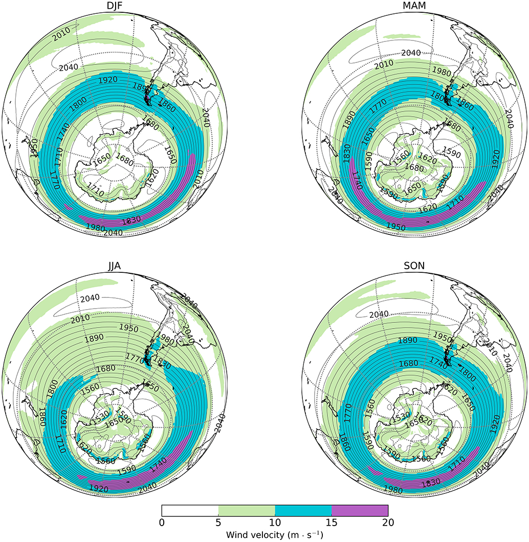
Figure 2. Mean wind velocity (colored areas) and geopotential height (contour lines) of 800 hPa from 1979 to 2017 obtained from ERA-Interim subdivided into seasons. An isohypse is plotted every 30 m. The interval of the meridians and parallels is 30°.

The Pacific Ocean is free from topographic disturbances. High wind velocities are present even in lower levels and the westerly wind belt almost coincides with the jet axis at approximately 50°S (Figure 3). The highest 10 m mean wind velocities (~15 m s⁻¹) occur at the Antarctic coast. Strong Antarctic outflow is present at the Bellingshausen and Amundsen Sea with its minimum in the austral summer months. Only on extreme rare occasions does a meridional circulation cause blocking of the west wind drift (Trenberth and Mo, 1985). Hence, the prevailing westerlies permanently advect moist air from the Pacific Ocean toward the southern tip of South America. This makes the southern Andes cordillera the only obstacle for the embedded baroclinic waves.

FIGURE 3

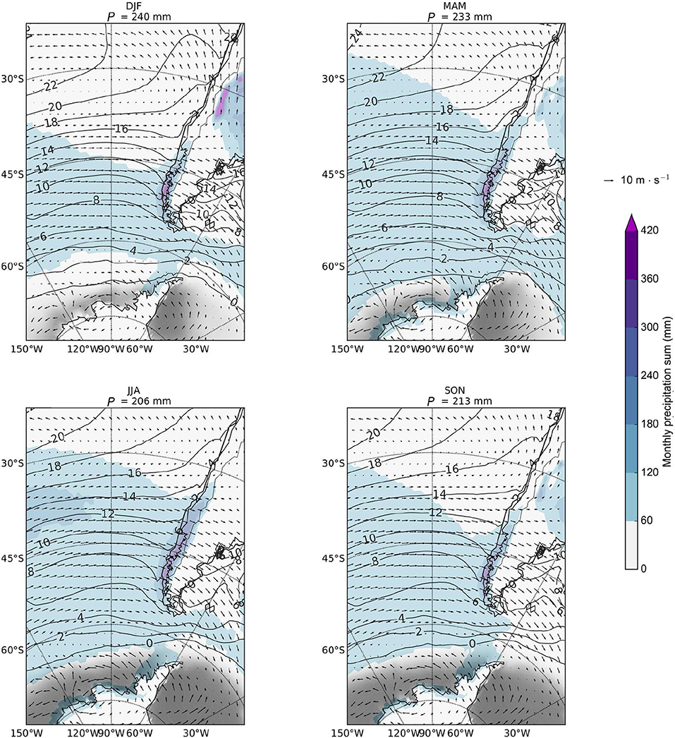
Figure 3. Seasonal precipitation (blue contours in mm per month), 10 m wind field (arrows with reference arrow), sea surface temperature (contour lines, 2 K interval) and sea ice cover (gray shaded area) from ERA-Interim (1979–2017). The corresponding monthly mean precipitation sum P accumulated over the target area is written in the header.

The north-south oriented Andes mountain ridge intersects the westerlies forming a pronounced climatic wall with very moist conditions on its upstream side and very dry conditions on the lee-side (Weischet, 1996; Schneider and Gies, 2004; Smith and Evans, 2007; Garreaud et al., 2009, 2013). Upstream of the mountain ridge orographic enhanced uplift leads to high accumulation rates of precipitation. The orography enhances the precipitation at the icefield. The amount of orographic precipitation in a stable flow depends, among other factors, on the strength of the crossbarrier flow U, the terrain height H, and the thermodynamic stability of the oncoming flow quantified by the Brunt-Väisälä Frequency N, and can be summarized in a non-dimensional ratio U(NH)⁻¹. It is often referred to as Froude number (or the inverse non-dimensional mountain height), which determines the flow regime (Houze, 2012). Past studies findings show a correlation between u and precipitation in west Patagonia (Schneider et al., 2003; Garreaud et al., 2013). The crossbarrier flow is one of three main drivers to describe the flow over a terrain and thus reasonable to correlate with the orographic precipitation.

Estimates of annual mean precipitation at the icefield range from 5,000 to 10,000 mm (Miller, 1976; DGA, 1987; Carrasco et al., 2002; Garreaud et al., 2013). Firn core measurements indicate extremely high accumulation rates. For example, net annual accumulation at glacier Tyndall, located at the southernmost part of the icefield, is 11,000–17,800 mm water equivalent (Shiraiwa et al., 2002). By contrast, only a few dozen kilometers downstream, the annular mean precipitation decreases to 300 mm (Garreaud et al., 2013). This west-east precipitation gradient is the most intense one worldwide (Schneider et al., 2003; Garreaud et al., 2013) and can be quantified with the drying ratio. The drying ratio describes the fraction of water vapor which rains out while passing a mountainous barrier. Smith and Evans (2007) estimated drying ration≈0.56 in the southern Andes (40 to 48°S), the highest value yet found to date in a mountain range.

The precipitation accumulated over the target region amounts 220 mm per month on median obtained from ERA-Interim. The monthly variation of the amount of precipitation hardly shows any seasonality (Figure 4). Warmer austral summer (DJF) and autumn (MAM) months indicate slightly more precipitation (P_{DJF, median} = 233 mm per month and P_{MAM, median} = 232 mm per month) than colder winter (JJA) months (P_{JJA, median} = 198 mm per month). But austral winter months show the highest variation of the monthly mean precipitation in the target region indicated by the inner-quartile range of 96 mm per month. During spring (SON) the median of the monthly mean precipitation accounts 213 mm per month. Note, the monthly resolved precipitation accumulated over the target area shows only the absolute amount, and is not a measurement for the intensity and frequency of individual precipitation events.

FIGURE 4

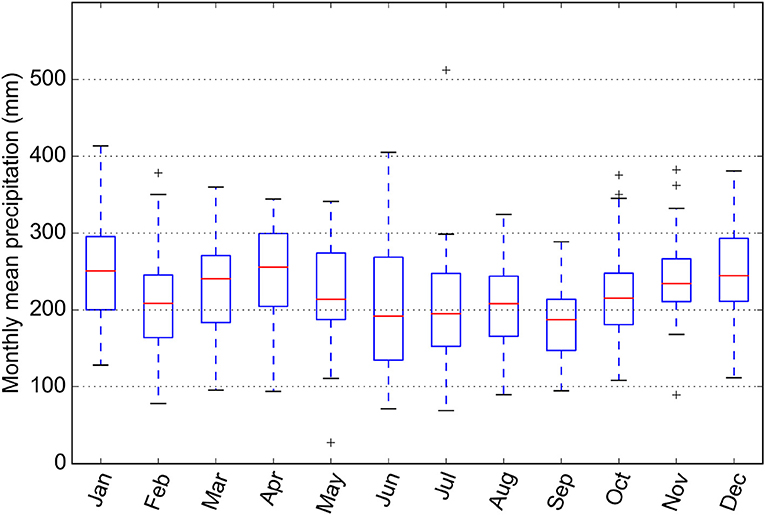
Figure 4. Monthly precipitation accumulated over the target area obtained from ERA-Interim (1979–2017).

The ERA-Interim model topography reaches from the sea surface to 1.011 m msl with an average of 595 m msl (Figure 1a). Only a few long term precipitation records are present in the vicinity of the icefield (Figure 1b). The automatic weather stations (AWS) “Amalia” and “Puerto Eden” are situated upstream of the icefield. The mean precipitation amounts significantly (p-value < 0.002) correlate with the ERA-Interim reanalysis (r_Pearson = 0.65 to 0.70) after the annual cycle is removed. They register a monthly mean sum of 255 mm at Amalia and 249 mm of Eden, respectively. Downstream of the icefield the AWS “Torres del Paine” provides 14 years of measurements. The monthly mean observations, obtained from http://explorador.cr2.cl/, correlate positively with the ERA-Interim data (r_Pearson = 0.68, p-value = 3.5e-26). The averaged monthly mean amounts to 64 mm, about a quarter of the upstream values. The AWS report a strong decreasing precipitation amount going from west to east across the cordillera. The ERA-Interim re-analysis data reproduces the precipitation features of southernmost South America in a temporal and spatial sense but a validation of the amounts of precipitation is impossible in absence of reliable observations. Extreme high wind velocities, with 10 m s⁻¹ on average, and snow events cause an under-catch of the rain gauges especially upstream of the cordillera e.g. AWS Puerto Eden, where the monthly mean observations are lower than the ERA-Interim data (Figure 1b) and the root-mean-square error indicate a deviation of RMSE_{Puerto Eden} = 154 mm. In general, global re-analysis data tends to underestimate the amount of precipitation in southern South America (Ward et al., 2011; Lenaerts et al., 2014). This feature is also observed by the station Amalia (RMSE_Amalia = 80 mm) and Puerto Eden (RMSE_{Torres del Paine} = 48 mm).

4. Results

4.1. Moisture Sources for the Southern Patagonia Icefield From 1979 to 2017

The mean moisture sources are derived from the Lagrangian methodology and represent the mean moisture uptake (in mm per month) within the scaled PBL, which contributes to the monthly precipitation in the icefield averaged over the time period from February 1979 to January 2017 (Figure 5). This plot contains 2,972,903 18-day backward trajectory calculations. The identified moisture sources are interpolated on a regular 1.5° grid.

FIGURE 5

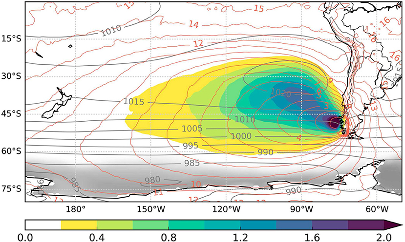
Figure 5. Mean moisture sources of the Southern Patagonia Icefield (colored area) in mm per month. Only moisture sources within the scaled PBL are considered. The maximal moisture uptake is 3.16 mm per month. The red lines indicate the mean travel time of the trajectories toward the icefield in days before arrival. The averaged mean sea level pressure (gray lines) and sea ice cover (gray shaded area) are depicted as well.

The majority of the moisture uptake originates from the South Pacific Ocean. The absolute maximum of 3.16 mm per month is close to the coast line of West Patagonia from where it takes about 1 day to reach the icefield. In that region the moisture transport time is about 1 day. Moisture source regions, which contribute more than 1 mm per month, reach to the subtropics. Within this region the transport of moisture takes up to 6 days from the source to the precipitation at the icefield. Significant moisture source regions southward of 60°S and in the Atlantic Ocean are absent. The contribution of moisture to the precipitation at the icefield from within the scaled PBL (evaporation from the surface) is 71%. At the trajectory ending position is already 4% of moisture included and 25% originate above the scaled PBL (see also Table S1 in Supplementary Material). The origin of this moisture is unknown and excluded in Figure 5.

At the trajectory ending position (t = −18 d) 75% of the trajectories are above the median of the scaled h_PBL (Figure 6a). From −18 days to −2 days, the median trajectory pressure level decreases from 703 hPa to 905 hPa. The moisture content within the trajectory increases from 2.0 g kg⁻¹ at −18 days to 4.8 g kg⁻¹ at t = −12 h (blue line, Figure 6b). Most of the trajectories are located within the scaled h_PBL from t = −4 d to arrival. During that time interval the largest six-hourly moisture uptake within the PBL contributes with Δq_median = 0.024 g kg⁻¹ to the precipitation at the icefield. The moisture change along the trajectory above the scaled PBL is about 1/3 of the moisture change within the scaled PBL. From t = −1 d to arrival we see an overall lifting of the trajectories to 835 hPa (on median). Since moisture decrease for all trajectories in the last 6 hours before reaching the icefield the moisture uptake is 0 g kg⁻¹ at −6 h to 0 h. Note that only the trajectories were selected, for which RH > 80% and Δq < 0 during t = −6 h to 0 h. Trajectories above the Antarctic continent originate from higher levels [p_traj(t > 13 d) ≤ 600 hPa] (Figure 7). Above the central Andes they reach mean heights of up to 500 hPa. Over the South Pacific Ocean a west-east gradient is visible with higher mean trajectory elevations in the west.

FIGURE 6

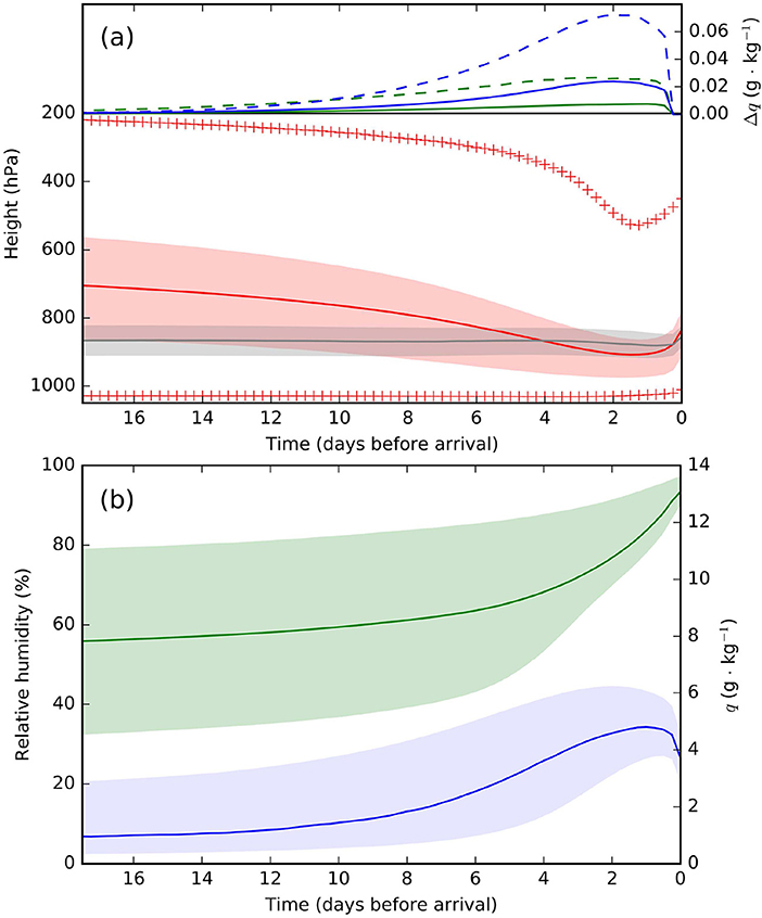
Figure 6. Vertical cross section of the trajectories. (a) (Bottom) Mean pressure height, quartiles and extremes (red), and the scaled boundary layer height (gray). (Top) Changes of the weighted specific humidity of moisture uptake within the scaled planetary boundary layer (PBL) (blue) and above the scaled PBL (green), which contribute to the precipitation at the icefield. Dashed lines show the corresponding upper quartile. (b) Quartiles and mean of relative humidity (green) and specific humidity (blue) of the trajectories.

FIGURE 7

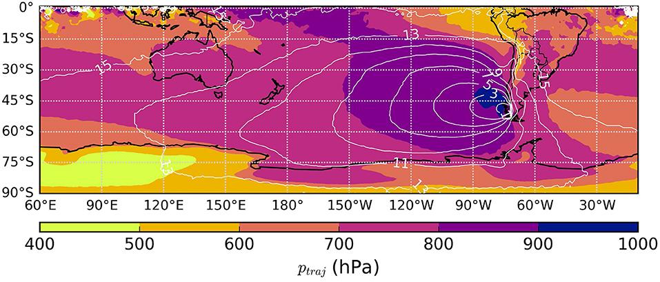
Figure 7. Mean pressure height of the trajectories interpolated on a 1.5° regular grid. White lines indicate the mean transport time of the moisture toward the Southern Patagonia Icefield in days before arrival.

The trajectories are very dry (RH < 20%) at the subtropical west coast of South America and Africa (Figure 8) due to subsidence. Very humid parts of the trajectories (RH > 80%) are present in the tropics and in the southeastern Pacific Ocean. The trajectories naturally cluster in the vicinity of the starting location of the icefield. The gradient of the number of trajectories per grid point is stronger in north-south than in west-east direction. Some regions show an absence of trajectories (white areas). During the whole calculation period not even one trajectory reached central Africa for instance.

FIGURE 8

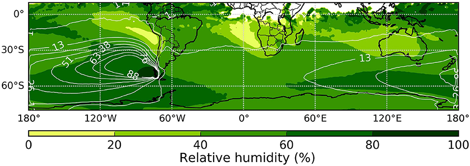
Figure 8. Mean relative humidity RH of the trajectories interpolated on a 1.5° regular grid. White contour lines present the averaged number of trajectories per grid point. White areas indicate a lack of information due to absence of trajectories.

4.2. Moisture Source Anomalies

4.2.1. Seasonal Variation

Seasons influence the moisture sources of the icefield (Figures 9a–d). Orange areas highlight a loss and green areas a surplus of the moisture source relative to the long-term annual climatological mean (1979–2017, Figure 5). A dipole like pattern is visible comparing the moisture source anomalies of JJA with DJF months, and MAM with SON months. The moisture uptake is reduced by 0.55 mm per month in the eastern South Pacific in the months DJF (Figure 9a). There is a moisture source deficit northwards and southwards of the icefield. By contrast there are positive anomalies along the 45°S parallel (0.5–0.25 mm per month). The 800 hPa geopotential height rises about 30 m in the central South Pacific which enhances the westerlies from 45 to 60°S parallel. Enhanced anticyclonic flow occurs in the subtropics. The geopotential height anomaly over the Ross Sea is 80 m, concomitant with a weakening of the westerlies in the proximity of Antarctica.

FIGURE 9

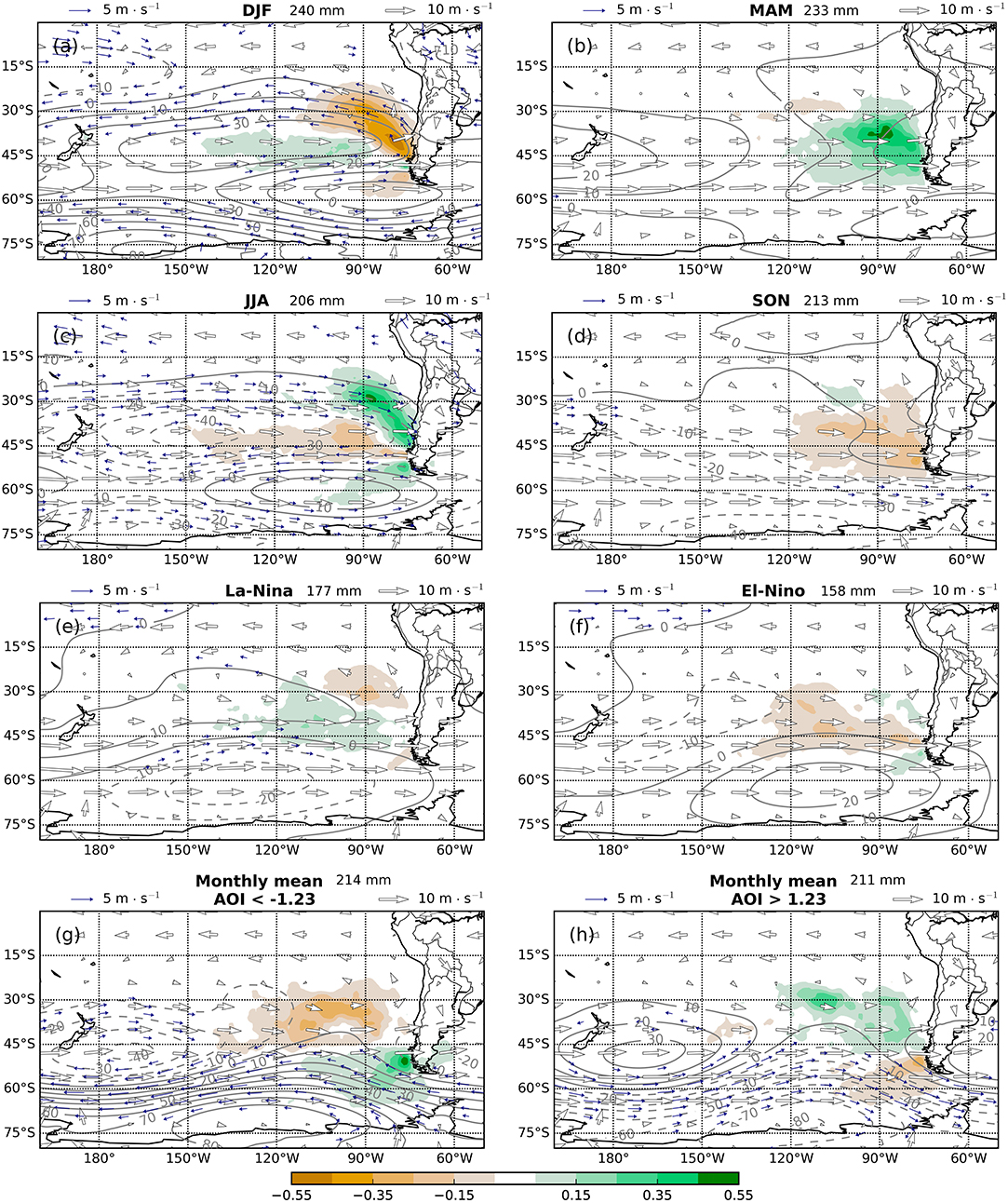
Figure 9. Significant (p < 0.05) moisture source anomalies (shaded areas in mm per month) derived from the climatological mean (1979–2017, Figure 5). Also shown are the geopotential height field anomalies at 800 hPa level in m (solid and dashed lines), wind field anomalies (> 1.5 m s⁻¹, blue arrows), and the mean wind field at 800 hPa level (white arrows with reference arrow). The anomalies are given for different seasons (a–d), La-Niña (e), El-Niño (f), strong negative (g), and positive (h) Antarctic oscillation index (AOI). Orange areas highlight lower, green areas a higher than average contribution to icefield precipitation from the evaporative moisture sources within the scaled PBL. The header includes the monthly mean precipitation in the target region.

The austral winter months (Figure 9c) show an inverted situation of the moisture source and geopotential height anomalies. In the eastern South Pacific northward of the icefield the monthly mean moisture sources increases to up to 0.55 mm per month. There is a deficit along the 45°S parallel, with the most pronounced region in the eastern South Pacific Ocean (up to −0.25 mm per month). An up to 40 m lower geopotential height decreases the negative poleward oriented gradient. In fact lower wind velocities occur upstream of the icefield at 800 hPa. The south-western part of the South Atlantic Ocean contributes up to 0.15 mm per month more to the precipitation at the icefield. MAM and SON months show small wind field anomalies (≤ 1.6 m s⁻¹) (Figures 9b,d). Despite small wind field anomalies those seasons show contrary moisture source anomalies. The MAM months show a positive evaporative moisture source anomaly in the eastern South Pacific of up to 0.55 mm per month. SON months show moisture source anomalies from −0.35 to 0.15 mm per month.

4.2.2. El-Nioño Southern Oscillation and Antarctic Oscillation Teleconnections

Beside seasons, determine large scale flow anomalies in the atmosphere the moisture sources of the icefield. A period of at least five consecutive overlapping 3-month seasons must exceed (deceed) an Ocean Niño Index (ONI) threshold of 0.5 (−0.5) in order to be classified as a full-fledge El-Niño (La-Niña) episode (National Oceanic and Atmospheric Administration, 2017). Considering these definitions, the time period from February 1979 to January 2017 contains 126 El-Niño and 90 La-Niña months (also see Figures S1, S2 in Supplementary Material). Both phenomenas have a similar seasonal distribution (Figure 10). Nevertheless, the annual cycle is considered in Figures 9e–h by subtracting the monthly climatology for each month respectively.

FIGURE 10

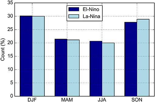
Figure 10. Seasonal distribution of El-Niño and La-Niña months relative to their respective totals.

El-Niño Southern Oscillation (ENSO) periods have moisture source anomalies of up to 0.35 mm per month (Figures 9e,f). La-Niña related positive anomalies of up to 0.25 mm per month occur in the central South Pacific Ocean between 30 and 45°S (Figure 9e). Up to 0.25 mm per month lower contributions appear in the subtropics at 30°S, 90°W. During El-Niño events, the moisture source decreases by 0.25 mm per month in the east South Pacific along the 45°S parallel (Figure 9f). Slightly more moisture of up to 0.15 mm per month originates from the east South Pacific Ocean northward and southward of the icefield. La-Niña (El-Niño) months indicate a lower (higher) geopotential height of up to 20 m at the South Pacific Ocean around 60°S, 120°W. The largest 800 hPa wind field anomalies appear in the tropical west Pacific. La-Niña (El-Niño) months show 2 m s⁻¹ stronger (weaker) easterlies, and depict the typical ENSO feature in the equatorial band.

A subset of months with standardized monthly mean Antarctic Oscillation index (AOI) falling the 10 percentile (AOI < −1.27) and exceeding the 90 percentile (AOI > 1.27) during the time period from February 1979 to January 2017 is taken to investigate Antarctic Oscillation dependent moisture source variations. Strong negative AOI months have up to 0.35 mm per month lower moisture uptake between 30 and 45°S in the east South Pacific, whereas moisture uptake from the ocean PBL in the proximity of the southern tip of South America is enhanced. Geopotential height anomalies weakens the westerly wind belt between 45 and 65°S in the South Pacific. Strong positive AOI months show stronger westerlies. Up to 0.35 mm per month more moisture originates from the mid-latitudes to the subtropics. The moisture sources in between 45 and 65°S show a deficit.

4.2.3. Extreme Events

The moisture source variability with respect to climatic extreme precipitation events is investigated. For purpose, we selected months with precipitation above the 90 percentile and below the 10 percentile, respectively, accumulated over the icefield obtained from the whole ERA-Interim data set. These selection represents dry (P_median = 343 mm) and humid (P_median = 111 mm) months.

Dry months are characterized by a 60 m increase of the geopotential height in the Drake Passage and 30 m lower geopotential heights over the South Pacific Ocean between 30 and 45°S. The lower meridional geopotential height gradient leads to weaker westerlies, an enhanced northerly flow at the west Patagonian coast, and have a deficit in the major moisture source region (Figure 11a). They contribute 0.15 mm per month less moisture just off the coastline of the icefield. A shift of the moisture source toward the south-west South Atlantic Ocean is apparent. This moisture source contributes up to 0.15 mm per month to the precipitation at the icefield. Dry months show up to 0.3 mm per month more moisture uptake over the South American continent where trajectories need on average less time (approximately 4 days; not shown) to reach the icefield.

FIGURE 11

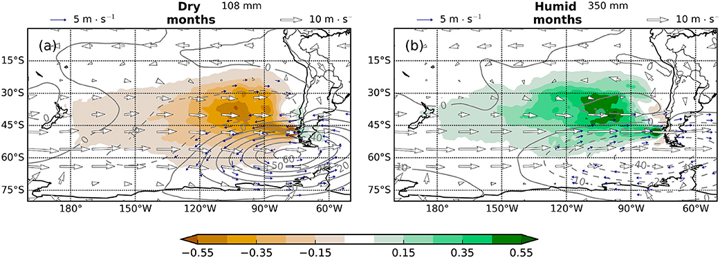
Figure 11. Significant (p < 0.05) moisture source anomalies (shaded areas in mm per month). Also shown are the geopotential height field anomalies at 800 hPa (in m; solid and dashed lines), wind field anomalies (> 1.5 m s⁻¹, blue arrows), and the mean wind field at 800 hPa level (white arrows). The anomalies are given for extremely (a) dry (10 percentile) and (b) humid (90 percentile) months. The minimum of the moisture uptake is −1.07 mm per month and maximum 0.90 mm per month respectively. The header includes the monthly mean precipitation in the target region.

During humid months the Drake Passage shows a 40 m decrease and in the subtropics a 10 m increase of the geopotential height in 800 hPa. The stronger poleward decreasing gradient of the 800 hPa geopotential height strengthens the westerlies. Trajectories which originate from southern South America, parts of the subtropical east South Pacific and the south-west South Atlantic in vicinity of the South American continent, need longer (approximately 12–15 days; not shown) to reach the icefield. There are negative anomalies (-0.15 mm per month) just off the coast line of South America. In the major moisture source region an overall increase of moisture uptake (up to 0.90 mm per month) is visible (Figure 11b).

An almost contrary pattern show the geopotential height anomaly of 800 hPa and the moisture source anomaly. The indicated anomalies in between the climatic extreme precipitation months have a dipole-like character. As before the annual cycle is taken into account.

The sea surface temperature and the mean sea level pressure anomaly are shown in Figure S3. The 800 hPa geopotential height and wind velocity (Figure S4), and the moisture sources (Figures S5–S8) are depicted as well.

5. Discussion

5.1. Major Evaporative Sources

The South Pacific Ocean is the major moisture source of the icefield in the 38 year climatology (Figure 5). The main moisture sources are located around 45°S and extend from 160°W to the west coast of South America. Those uptake regions appear a few degrees northward of the circumpolar vortex. There is a region of cyclogenesis at approximately 170°W in the proximity of New Zealand (Taljaard, 1968). In addition, along 45°S baroclinic instabilities exist due to the polar front. These features explain the longitudinal extent of the moisture sources close to New Zealand at 45°S and their location a few degrees northward of the westerly wind belt.

The prevailing westerlies in the high southern latitudes cause a high trajectory density, count of trajectories per grid point, upstream of the target region (Figure 8), which is responsible for the moisture uptake maximum in a small region just off the coast line of west Patagonia. On the one hand the moisture uptake of each trajectory add up at the same grid point. On the other hand, uptake regions closer to the target have greater influence. They achieve a higher contribution due to less en route precipitation in comparison with identified uptake regions several days before arrival.

Moisture uptake regions extend to the subtropics and make an important contribution to the precipitation at the icefield. This highlights the role of the subtropical high pressure system in terms of the moisture origin of the icefield. In the Subtropics downstream of the Andes relatively dry air masses descend. Under the influence of the anticyclonical flow the air masses reach low heights (Figure 7) and moisten with the Pacific PBL (Figure 8). The air masses travel polwards into the mid-latitudes, where they come into the influence of the strong westerly storm track and finally reach the icefield. Pfahl et al. (2014) identified a moisture source in the subtropical South Pacific of warm conveyor belts. The importance of the warm conveyor belts in association with the regional precipitation at the icefield remains unknown in the present results.

The stationary high pressure region in the middle of Antarctica characterizes the circulation features at the coast of the continent (Figure 2). A closer examination of the 10 m wind shows the characteristics of the katabatic outflow (Figure 3). High offshore wind velocities occur close to the surface at Bellingshausen Sea, Amundsen Sea, and Ross Sea. Trajectories from those regions originate from the lower troposphere and indicate a subsidence at the transition from the continent to the South Pacific Ocean (Figure 7). The dominant mechanism for the offshore air flow in the Bellingshausen and Amundsen Sea is the persistent low pressure system in the Ross Sea (Papritz et al., 2015). This location is characterized by having the lowest mean sea level pressure of the South Pacific (Figure 5). If the cold and dry air masses from the inner Antarctic Continent are advected equatorwards across the sea ice shelfs over the relatively warm and moist ocean (cold air outbreaks), they can trigger convection and PBL fronts (Drüe and Heinemann, 2001). Thus the Ross, Amundsen and Bellingshausen Sea have a high density of mesocyclones (Irving et al., 2010). Seasonal trends of mesoscale cyclone activity over the ice-free southern ocean from 1999 to 2008 show an agreement with the examined seasonal moisture source anomaly. For instance, the ERA-Interim re-analysis data shows the strongest mean outflow off Antarctica during MAM and JJA (Figure 3) when Irving et al. (2010) indicate the highest density of mesocyclones in the Amundsen and Bellingshausen Sea. The moisture sources during this time period display positive anomalies south of 50°S (Figures 9b,c). Specially during JJA the positive moisture source anomalies reach close to the Amundsen and Bellingshausen Sea. This could be an evidence for cold air outbreaks, which moisten inside the Pacific PBL and contribute to the precipitation at the icefield. The identified source regions in the southernmost South Pacific might be the result of polar lows and their strengthening of the storm track.

5.2. Transport Time of Moisture

A substantial amount of moisture needs <10 days from its origin to the icefield (Figure 5). The zonal moisture exchange is faster than the meridional due to the westerly wind belt. Trajectories have the highest density (Figure 8) and reach on average the highest velocities in vicinity of the jet axis. The highest moisture uptake occurs 2 days before arrival (Figure 6). At this point, the majority of the trajectories are located inside the scaled PBL. The day before arrival the trajectories show an overall lifting due to the orography. Beyond 10 days before arrival, backward trajectories originate from higher levels, and hence indicate higher moisture uptake rates above the scaled PBL. This contribution is negligible. The highest moisture loss of the trajectories is due to precipitation at icefield. The absence of obstacles in the Pacific Ocean leads to only small amounts of en route precipitation (compare averaged precipitation amounts in Figure 3).

5.3. Moisture Source Variabilities

Disturbances of the westerly wind belt, caused by baroclinic instabilities in the mid-latitudes, inject moist air masses from the tropics into the westerly wind belt. Thus, the westerlies are the dominant transport mechanism of moist air toward the icefield. A dislocation of the westerly wind belt leads to anomalies of precipitation (Garreaud et al., 2013), changes transport pathways of moisture toward the icefield and the location of moisture sources concerning the icefield. The contribution from the south-west South Atlantic Ocean is negligible. A substantial amount of moisture originates in the South Atlantic only in particular situations. One of the requirements is a positive geopotential height anomaly close to the Drake Passage (Figure 11). As a consequence, anticyclonic flow occurs over southern South America accompanied by a shift of the moisture sources to the south-east South Atlantic. The moisture uptake decreases in the major moisture source region between 40 and 50°S. Positive moisture source anomalies appear only in the vicinity of the southern South American coast. This phenomenon is more likely during El-Niño (Figure 9f) and JJA months (Figure 9c), and characterizes dry months (Figure 11a). Dry months are the most frequent during El-Niño and JJA (Figure 13), and thus they exhibit similar anomaly patterns. May 2016 shows the lowest accumulation rate of precipitation at the icefield in the whole ERA-Interim data and is used to point out those circulation features (Figure 12).

FIGURE 12

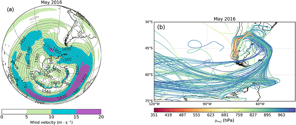
Figure 12. (a) ERA-Interim 800 hPa geopotential height and wind velocity from May 2016. (b) Sample of trajectories with moisture uptake in the south-west South Atlantic during May 2016. The color indicate their pressure height.

For May 2016 the averaged 800 hPa geopotential height indicates strongly meridional flow upstream of southern South America (Figure 12a). The high pressure ridge above southern South America causes an anticyclonic flow with the center at the southern South American continent. The polewards displacement of the storm track (positive geopotential height anomaly in the Drake Passage) forces the trajectories to travel through the Drake passage (Figure 12b). Anticyclonic curvature above the south-eastern South Atlantic Ocean moves the trajectories equatorwards. The air masses moisten inside the PBL of the Atlantic and the anticyclonic flow controls their westward flow over the continent. En route precipitation above the continent, with the maximum upstream of the Andes cordillera (see Supplementary Material Figure S9) due to orographic lifting, decreases the moisture source contribution of the South Atlantic but increases the intercontinental moisture recycling also visible in Figure 11a. Finally, meridional flow occurs along the coast line of west Patagonia. Trajectories within the Pacific PBL increase their moisture content and contribute to the positive moisture source anomaly along the western Patagonia coast. The strongly meridional flow at high southern latitudes in vicinity of the South American continent causes a low monthly precipitation sum at the icefield. This phenomenon is twice as frequent during austral winter compared to summer months (Figure 13 and Trenberth and Mo, 1985).

FIGURE 13

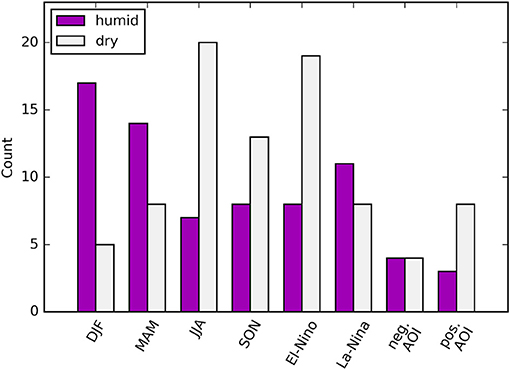
Figure 13. The count of humid (90 percentile) and dry (10 percentile) months grouped by seasons, El-Niño, La-Niña , negative and positive antarctic oscillation index (AOI).

By contrast, a strengthening of the zonal westerly flow in the south-east South Pacific increases the moisture uptake in the major moisture source region. During humid months (Figure 11b), DJF (Figure 9a), and La-Niña months (Figure 9e) the zonal flow around 50°S is most intense. Those months show a poleward shift of the subtropical anticyclone accompanied by a poleward shift of moisture sources from the subtropics to the mid-latitudes. In addition, a lower geopotential height at around 60°S increases the north-south pressure gradient between 45 and 60°S and results in a strengthening of the westerlies. As a consequence, long-range transport of moisture occurs with its maximal extent close to 180°W during humid months.

5.4. Variations of the Moisture Sources

Extreme precipitation events coincide with the strongest north-south pressure gradient anomaly between 45 and 60°S. Past studies emphasize a correlation between wind velocity and precipitation in west Patagonia (Schneider et al., 2003; Garreaud et al., 2013). The strength and location of the westerly wind belt controls the orographic precipitation at the icefield. The crossbarrier flow is one of three main drivers to describe the flow over a terrain and thus reasonable to correlate with the orographic precipitation. The main drivers can be summarized in a nondimensional ratio U(NH)⁻¹, which is often referred to as Froude number (or the inverse nondimensional mountain height), and determines the flow regime (Houze, 2012). Whenever the upstream Froude number is high (fast flow velocity, low stability, and/or a small mountain height), the airflow rises over the terrain. If the upstream Froude number is low (slow flow velocity, high stability and/or high mountains) the upcoming air is blocked and the flow is deflected laterally. In case of a narrow mountain ridge, high wind velocities and atmospheric conditions as observed in southernmost South America, the maximum of precipitation shifts from the hill top to the windward slope (Smith and Evans, 2007). Enhanced upstream precipitation at the icefield is also indicated by ERA-Interim and shown in Figure 3.

ERA-Interim reanalysis data indicate no significant monthly correlation between the ENSO phenomenon and the precipitation at the icefield (r_Pearson = −0.06, p-value = 0.34). The moisture source variability during ENSO months is half of the magnitude in comparison to the seasonal variation. El-Niño monthly evaporative moisture source anomalies show similarities to the austral winter months. La-Niña months show similarities to summer months. But both events show similar seasonal occurrence and thus only mirror the ENSO related anomalies. A direct link between SST anomalies in the South Pacific and moisture source anomalies does not exist.

The monthly mean precipitation at the icefield is independent of the AOI (r_Pearson = −0.06, p-value = 0.19). Strong negative AOI months show less moisture contribution from the subtropics and enhanced moisture uptake in the mid-latitudes (Figure 9g). A reduction of the westerly wind in the South Pacific decreases the moisture transport from the subtropics toward the icefield. Enhanced Antarctic outflow in the Bellingshausen and Amundsen Sea increases the moisture sources in the south-east South Pacific. Strong positive AOI months indicate an opposite pattern (Figure 9h). They show stronger westerly winds around 60°S. Less katabatic outflow from the Bellingshausen and Amundsen Sea results in a moisture source deficit in the south-east South Pacific. The north-westerly wind field anomalies in vicinity of the icefield increase the moisture uptake regions from the subtropics to 45°S.

5.5. Uncertainties

Evaporation or precipitation affect the net moisture change along a trajectory (Equation 1). We have omitted formation and dissolution of clouds and the amount of evaporative moisture source. Considering the specific cloud ice water content and the specific cloud liquid water content the whole amount of moisture sources decreases by approximately 5% (not shown). It has a negligible effect on the evaporation pattern. Furthermore, the applied moisture source detection technique neglects moisture changes due to convection. Especially in warmer regions, such as the tropics and subtropics, or due to cold air outbreaks in high southern latitudes, convection plays a major role. In those regions we expect lower accuracy of the detected moisture sources. Transport errors increase significantly for trajectory calculations beyond 10 days (Stohl and Seibert, 1998). We applied 18-day backward trajectory calculations and have to consider inaccurate trajectory ending positions. However, a longer backward trajectory calculation time period than 10 days is not necessary to examine the moisture sources of the icefield (Figure 5). This is in accordance with the average residence time of water in the atmosphere (Van Der Ent and Tuinenburg, 2017). Shorter backward calculation periods are recommended for upcoming studies.

6. Conclusion

An established moisture source detection technique (Sodemann et al., 2008) was applied to identify moisture sources for precipitation at the Southern Patagonia Icefield. The three-dimensional kinematic 18-day backward trajectories are based on ERA-Interim reanalysis data from January 1979 to January 2017. This method is able to quantify the water vapor origin, the transport time and the favored transport paths, and presents a diagnostic picture of moisture source regions of the icefield.

The major moisture source of the icefield is found in the South Pacific between 80 to 160°W and 30 to 60°S (Figure 5). We detected 71% of the moisture sources responsible for the precipitation at the icefield. The cause for the moisture uptake above the PBL (25%) and the moisture content already included at the trajectory ending position (4%) have not been investigated.

The maximum moisture uptake is located just off the coastline of west Patagonia. The largest contribution of moisture sources extends north up to the subtropics, where a persistent anticyclone centered around 100°W and 30°S exists. Moisture uptake regions in the subpolar regions have a smaller contribution. In the high southern latitudes, cold air outbreaks are likely the dominant mechanism for moisture uptake. Relatively cold and dry descending air masses become moistened in the relatively warm planetary boundary layer over the ice-free Southern Pacific. The rather instable situation of relatively cold air masses above the relatively warm sea surface initialize convection and enhance the baroclinity of the westerly storm track. Furthermore, moisture sources which coincide with the prevailing westerlies have the biggest westward extent to 160°W. This region shows the highest trajectory density and indicates the favored pathways of moist air masses (Figure 8).

In addition controlling the transport pathways, the location of the westerly wind belt determines the amount of precipitation and the moisture origin of the icefield (Figure 3 and Figure 11). In general, stronger westerly winds around 50°S lead to more long-range transport and enhanced moisture uptake from subtropics to mid-latitudes, and characterize climatic humid months (Figure 11b). By contrast, a weakening of the westerlies, and/or a poleward shift of the jet axis, is accompanied by enhanced moisture uptake along the southern tip of South America and less moisture supply from the subtropics and mid-latitudes in the central South Pacific (Figure 9g and Figure 11a). An appropriate proxy is an anomaly of the 800 hPa geopotential height extending from the Ross Sea to the Drake Passage. An extraordinarily strong positive anomaly of the geopotential height in the Drake Passage results in an anticyclonic flow over the southern tip of South America (Figure 12a). The high pressure ridge transports moisture from the south-western Atlantic above the Andes along the west Patagonians coast toward the icefield (Figure 12b). The north-westerly advection of moisture enhances the moisture source contribution from the subtropics only along the coast line. These events occur during climatologically drier months (Figure 11a).

Seasonal variation of moisture source regions exist. During MAM (Figure 9b) and JJA (Figure 9c) up to ~40 % more moisture originates from the subtropics. Austral summer months have enhanced moisture uptake in the mid-latitudes and less contribution from the subtropics (Figure 9a). The ENSO related moisture source anomalies are half as large as the seasonal anomalies. During La-Niña more moisture originates from the mid-latitude region of South Pacific due to enhanced westerlies (Figure 9e). Opposite behavior is exhibited by El-Niño months (Figure 9f). The Antarctic Oscillation related moisture source anomalies show a similar strength of anomalies as the seasonal anomalies. Months with a strong negative Antarctic Oscillation Index show less moisture sources between subtropics and mid-latitudes (Figure 9g). More moisture originates from high southern latitudes due to increased outflow from Bellingshausen and Amundsen Sea. By contrast, months with a strong positive Antarctic Oscillation Index show an opposite pattern in moisture source and geopotential height anomalies, due to the anomalous meandering geopotential pattern (Figure 9h).

The Lagrangian analysis of precipitation origins for the icefield considers en route precipitation. A large part of the moisture uptake in remote regions such as the Indian Ocean or the tropics does not reach the icefield since it is rained out during transport. Identified moisture sources outside the 10-day backward calculation time period have a negligible impact as expected due to the average residence time of water in the atmosphere (Van Der Ent and Tuinenburg, 2017). The moisture uptake is at its maximum 2 days before arrival, when the majority of air masses are inside the PBL (Figure 6a).

The Lagrangian perspective highlights the interplay between the large scale climate modes and moisture sources of the icefield. These findings may help to interpret anomalies of paleo-climatological records of isotopic composition obtained from lake sediments (e.g. Mayr et al., 2005), lakes or precipitation samples (e.g. Mayr et al., 2007), ice cores (e.g. Schwikowski et al., 2013), or vegetation (e.g. GrieSSinger et al., 2018), in Fuego-Patagonia where a direct link to ambient environmental changes is absent. Thus, the identified moisture sources are one more building block to interpret climate proxies at the icefield from 1979 to 2017. A companion paper compares the findings of the Lagrangian moisture source detection with tree-ring records from Perito Moreno (GrieSSinger et al., 2018). The comparison shows, that variations in the moisture sources influence the δ¹⁸O Tree-ring chronology of Nothofagus pumilio located in the vicinity of the Perito Moreno Glacier. A simultaneous study compares findings of the stable hydrogen and oxygen isotope composition of precipitation, and lake and river systems from different sites in southern South America with results of the moisture source detection method presented in this manuscript. They found that identified moisture sources and major transport pathways of moist air masses can clarify isotopic fractionation processes.

Author Contributions

LL implemented the trajectory model, prepared the figures and wrote the manuscript. TS initialized the idea of this study and supported the research with in-depth knowledge of the Southern Patagonia Icefield. GM was the supervisor at the University of Innsbruck and he provided all the necessary resources to deal with a comprehensive climatological study. All authors discussed the findings and participated in preparing the final manuscript.

Conflict of Interest Statement

The authors declare that the research was conducted in the absence of any commercial or financial relationships that could be construed as a potential conflict of interest.

Acknowledgments

We have to acknowledge the support of Michael Sprenger. His fundamental knowledge of technical details and willingness to help contributed to a successful application of LAGRANTO. We gratefully acknowledge financial support by the Deutsche Forschungsgemeinschaft (DFG), no. SA 2339/4-1. The study was conducted in the frame of the research area Alpiner Raum of the University of Innsbruck. The publication fund of the University of Innsbruck supported its publication.

Supplementary Material

The Supplementary Material for this article can be found online at: https://www.frontiersin.org/articles/10.3389/feart.2018.00219/full#supplementary-material

References

Aniya, M., Sato, H., Naruse, R., Skvarca, P., and Casassa, G. (1996). The use of satellite and airborne imagery to inventory outlet glaciers of the Southern Patagonia Icefield, South America. Photogr. Eng. Remote Sens. 62, 1361–1369. doi: 10.1175/2009MWR2881.1

CrossRef Full Text | Google Scholar

Barrett, B. S., Garreaud, R., and Falvey, M. (2009). Effect of the Andes cordillera on precipitation from a midlatitude cold front. Mon. Weather Rev. 137, 3092–3109.

Google Scholar

Berkelhammer, M. B., and Stott, L. D. (2008). Recent and dramatic changes in Pacific storm trajectories recorded in δ¹⁸O from Bristlecone Pine tree ring cellulose. Geochem. Geophys. Geosyst. 9:Q04008. doi: 10.1029/2007GC001803

CrossRef Full Text | Google Scholar

Berrisford, P., Dee, D., Poli, P., Brugge, R., Fielding, K., Fuentes, M., et al. (2011). The ERA-Interim archive Version 2.0. Reading: Shinfield Park.

Google Scholar

Bracegirdle, T. J. (2013). Climatology and recent increase of westerly winds over the Amundsen Sea derived from six reanalyses. Int. J. Climatol. 33, 843–851. doi: 10.1002/joc.3473

CrossRef Full Text | Google Scholar

Bracegirdle, T. J., and Marshall, G. J. (2012). The reliability of Antarctic tropospheric pressure and temperature in the latest global reanalyses. J. Clim. 25, 7138–7146. doi: 10.1175/JCLI-D-11-00685.1

CrossRef Full Text | Google Scholar

Bromwich, D. H., Nicolas, J. P., and Monaghan, A. J. (2011). An assessment of precipitation changes over Antarctica and the Southern Ocean since 1989 in contemporary global reanalyses. J. Clim. 24, 4189–4209. doi: 10.1175/2011JCLI4074.1

CrossRef Full Text | Google Scholar

Carrasco, J. F., Casassa, G., and Rivera, A. (2002). “Meteorological and climatological aspects of the Southern Patagonia Icefield,” in The Patagonian Icefields. Series of the Centro de Estudios Científicos (Boston, MA: Springer), 29–41.

Google Scholar

Dee, D., Uppala, S., Simmons, A., Berrisford, P., Poli, P., Kobayashi, S., et al. (2011). The ERA-Interim reanalysis: configuration and performance of the data assimilation system. Q. J. R. Meteorol. Soc. 137, 553–597. doi: 10.1002/qj.828

CrossRef Full Text | Google Scholar

DGA (1987). Balance Hídrico de Chile. Santiago: Dirección General de Aguas, 34.

Drüe, C., and Heinemann, G. (2001). Airborne investigation of arctic boundary-layer fronts over the marginal ice zone of the Davis Strait. Bound. -Layer Meteorol. 101, 261–292. doi: 10.1023/A:1019223513815

CrossRef Full Text | Google Scholar

Garreaud, R., Lopez, P., Minvielle, M., and Rojas, M. (2013). Large-scale control on the Patagonian climate. J. Clim. 26, 215–230. doi: 10.1175/JCLI-D-12-00001.1

CrossRef Full Text | Google Scholar

Garreaud, R. D., Vuille, M., Compagnucci, R., and Marengo, J. (2009). Present-day South American Climate. Palaeogeogr. Palaeoclimatol. Palaeoecol. 281, 180–195. doi: 10.1016/j.palaeo.2007.10.032

CrossRef Full Text | Google Scholar

Gat, J. R. (1996). Oxygen and hydrogen isotopes in the hydrologic cycle. Annu. Rev. Earth Planet. Sci. 24, 225–262. doi: 10.1146/annurev.earth.24.1.225

CrossRef Full Text | Google Scholar

GrieSSinger, J., Langhamer, L., Schneider, C., SaSS, B.-L., Steger, D., Skvarca, P., et al. (2018). Imprints of climate signals in a 204 year δ¹⁸O tree-ring record of Nothofagus pumilio from Perito Moreno Glacier, Southern Patagonia (50°S). Front. Earth Sci. 6:27. doi: 10.3389/feart.2018.00027

CrossRef Full Text | Google Scholar

Houze, R. A. (2012). Orographic effects on precipitating clouds. Rev. Geophys. 50:RG1001. doi: 10.1029/2011RG000365

CrossRef Full Text | Google Scholar

Irving, D., Simmonds, I., and Keay, K. (2010). Mesoscale cyclone activity over the ice-free Southern Ocean: 1999–2008. J. Clim. 23, 5404–5420. doi: 10.1175/2010JCLI3628.1

CrossRef Full Text | Google Scholar

Lenaerts, J. T., Van Den Broeke, M. R., van Wessem, J. M., van de Berg, W. J., van Meijgaard, E., van Ulft, L. H., et al. (2014). Extreme precipitation and climate gradients in Patagonia revealed by high-resolution regional atmospheric climate modeling. J. Clim. 27, 4607–4621. doi: 10.1175/JCLI-D-13-00579.1

CrossRef Full Text | Google Scholar

Mayr, C., Fey, M., Haberzettl, T., Janssen, S., Lücke, A., Maidana, N. I., et al. (2005). Palaeoenvironmental changes in southern Patagonia during the last millennium recorded in lake sediments from Laguna Azul (Argentina). Palaeogeogr. Palaeoclimatol. Palaeoecol. 228, 203–227. doi: 10.1016/j.palaeo.2005.06.001

CrossRef Full Text | Google Scholar

Mayr, C., Lücke, A., Stichler, W., Trimborn, P., Ercolano, B., Oliva, G., et al. (2007). Precipitation origin and evaporation of lakes in semi-arid Patagonia (Argentina) inferred from stable isotopes (δ 18 O, δ 2 H). J. Hydrol. 334, 53–63. doi: 10.1016/j.jhydrol.2006.09.025

CrossRef Full Text | Google Scholar

Merlivat, L., and Jouzel, J. (1979). Global climatic interpretation of the deuterium-oxygen 18 relationship for precipitation. J. Geophys. Res. 84, 5029–5033. doi: 10.1029/JC084iC08p05029

CrossRef Full Text | Google Scholar

Miller, A. (1976). The climate of Chile. World Survey Climatol. 12, 113–145.

National Oceanic Atmospheric Administration (2017). ENSO: Recent Evolution, Current Status and Predictions. Avaialble online at: http://www.cpc.ncep.noaa.gov/products/analysis_monitoring/lanina/enso_evolution-status-fcsts-web.pdf (Accessed March 10, 2017).

Newell, R. E., Newell, N. E., Zhu, Y., and Scott, C. (1992). Tropospheric rivers?–A pilot study. Geophys. Res. Lett. 19, 2401–2404. doi: 10.1029/92GL02916

CrossRef Full Text | Google Scholar

Nicolas, J. P., and Bromwich, D. H. (2011). Precipitation changes in high southern latitudes from global reanalyses: a cautionary tale. Surveys Geophys. 32, 475–494. doi: 10.1007/s10712-011-9114-6

CrossRef Full Text | Google Scholar

Papritz, L., Pfahl, S., Sodemann, H., and Wernli, H. (2015). A climatology of cold air outbreaks and their impact on air–sea heat fluxes in the high-latitude South Pacific. J. Clim. 28, 342–364. doi: 10.1175/JCLI-D-14-00482.1

CrossRef Full Text | Google Scholar

Persson, A. (2015). User Guide to ECMWF Forecast Products. Reading: ECMWF.

Pfahl, S., Madonna, E., Boettcher, M., Joos, H., and Wernli, H. (2014). Warm conveyor belts in the ERA-Interim dataset (1979–2010). Part II: Moisture origin and relevance for precipitation. J. Clim. 27, 27–40. doi: 10.1175/JCLI-D-13-00223.1

CrossRef Full Text | Google Scholar

Rivadeneira, M. C. (2011). Natural Variability of the Atmospheric Composition and Anthropogenic Influence in Patagonia : Contribution to the Understanding of Transport Pathways Along the Equator - Mid latitudes - Pole Transect. Ph.D. dissertation, Université de Grenoble, Montpellier.

Scheele, M., Siegmund, P., and Van Velthoven, P. (1996). Sensitivity of trajectories to data resolution and its dependence on the starting point: in or outside a tropopause fold. Meteorol. Appl. 3, 267–273. doi: 10.1002/met.5060030308

CrossRef Full Text | Google Scholar

Schneider, C., and Gies, D. (2004). Effects of El Niño–southern oscillation on southernmost South America precipitation at 53 S revealed from NCEP–NCAR reanalyses and weather station data. Int. J. Climatol. 24, 1057–1076. doi: 10.1002/joc.1057

CrossRef Full Text | Google Scholar

Schneider, C., Glaser, M., Kilian, R., Santana, A., Butorovic, N., and Casassa, G. (2003). Weather observations across the southern Andes at 53 S. Phys. Geogr. 24, 97–119. doi: 10.2747/0272-3646.24.2.97

CrossRef Full Text | Google Scholar

Schwikowski, M., Schläppi, M., Santibañez, P., Rivera, A., and Casassa, G. (2013). Net accumulation rates derived from ice core stable isotope records of Pío XI glacier, Southern Patagonia Icefield. Cryosphere 7, 1635–1644. doi: 10.5194/tc-7-1635-2013

CrossRef Full Text | Google Scholar

Shiraiwa, T., Kohshima, S., Uemura, R., Yoshida, N., Matoba, S., Uetake, J., et al. (2002). High net accumulation rates at Campo de Hielo Patago´ nico Sur, South America, revealed by analysis of a 45.97 m long ice core. Ann. Glaciol. 35, 84–90. doi: 10.3189/172756402781816942

CrossRef Full Text | Google Scholar

Smith, R. B., and Evans, J. P. (2007). Orographic precipitation and water vapor fractionation over the southern Andes. J. Hydrometeorol. 8, 3–19. doi: 10.1175/JHM555.1

CrossRef Full Text | Google Scholar

Sodemann, H., Schwierz, C., and Wernli, H. (2008). Interannual variability of Greenland winter precipitation sources: Lagrangian moisture diagnostic and North Atlantic Oscillation influence. J. Geophys. Res. 113:D03107. doi: 10.1029/2007JD008503

CrossRef Full Text | Google Scholar

Sprenger, M., and Wernli, H. (2015). The LAGRANTO Lagrangian analysis tool–version 2.0. Geosci. Model Dev. 8, 2569–2586. doi: 10.5194/gmd-8-2569-2015

CrossRef Full Text | Google Scholar

Steen-Larsen, H. C., Johnsen, S. J., Masson-Delmotte, V., Stenni, B., Risi, C., Sodemann, H., et al. (2013). Continuous monitoring of summer surface water vapor isotopic composition above the Greenland Ice Sheet. Atmos. Chem. Phys. 13, 4815–4828. doi: 10.5194/acp-13-4815-2013

CrossRef Full Text | Google Scholar

Stohl, A., Haimberger, L., Scheele, M., and Wernli, H. (2001). An intercomparison of results from three trajectory models. Meteorol. Appl. 8, 127–135. doi: 10.1017/S1350482701002018

CrossRef Full Text | Google Scholar

Stohl, A., and James, P. (2004). A Lagrangian analysis of the atmospheric branch of the global water cycle. Part I: Method description, validation, and demonstration for the August 2002 flooding in central Europe. J. Hydrometeorol. 5, 656–678. doi: 10.1175/1525-7541(2004)005<0656:ALAOTA>2.0.CO;2

CrossRef Full Text | Google Scholar

Stohl, A., and Seibert, P. (1998). Accuracy of trajectories as determined from the conservation of meteorological tracers. Q. J. R. Meteorol. Soc. 124, 1465–1484. doi: 10.1002/qj.49712454907

CrossRef Full Text | Google Scholar

Taljaard, J. (1968). Climatic frontal zones of the Southern Hemisphere. Notos 17, 23–39.

Trenberth, K. F., and Mo, K. C. (1985). Blocking in the southern hemisphere. Mon. Weath. Rev. 113, 3–21. doi: 10.1175/1520-0493(1985)113<0003:BITSH>2.0.CO;2

CrossRef Full Text | Google Scholar

Van Der Ent, R. J., and Tuinenburg, O. A. (2017). The residence time of water in the atmosphere revisited. Hydrol. Earth Syst. Sci. 21:779. doi: 10.5194/hess-21-779-2017

CrossRef Full Text | Google Scholar

Viale, M., Houze, R. A. Jr, and Rasmussen, K. L. (2013). Upstream orographic enhancement of a narrow cold-frontal rainband approaching the Andes. Mon. Weath. Rev. 141, 1708–1730. doi: 10.1175/MWR-D-12-00138.1

CrossRef Full Text | Google Scholar

Viale, M., and Nuñez, M. N. (2011). Climatology of winter orographic precipitation over the subtropical central Andes and associated synoptic and regional characteristics. J. Hydrometeorol. 12, 481–507. doi: 10.1175/2010JHM1284.1

CrossRef Full Text | Google Scholar

Ward, E., Buytaert, W., Peaver, L., and Wheater, H. (2011). Evaluation of precipitation products over complex mountainous terrain: a water resources perspective. Adv. Water Resour. 34, 1222–1231. doi: 10.1016/j.advwatres.2011.05.007

CrossRef Full Text | Google Scholar

Weischet, W. (1996). Regionale Klimatologie Teil 1. Stuttgart: Schweizerbart Science Publishers.

Google Scholar

Wernicke, J., Hochreuther, P., Grießinger, J., Zhu, H., Wang, L., and Bräuning, A. (2017). Air mass origin signals in δ¹⁸O of tree-ring cellulose revealed by back-trajectory modeling at the monsoonal Tibetan plateau. Int. J. Biometeorol. 61, 1109–1124. doi: 10.1007/s00484-016-1292-y

CrossRef Full Text | Google Scholar

Wernli, B. H., and Davies, H. C. (1997). A Lagrangian-based analysis of extratropical cyclones. I: the method and some applications. Q. J. R. Meteorol. Soc. 123, 467–489. doi: 10.1002/qj.49712353811

CrossRef Full Text | Google Scholar

Winschall, A., Pfahl, S., Sodemann, H., and Wernli, H. (2014). Comparison of Eulerian and Lagrangian moisture source diagnostics–the flood event in eastern Europe in May 2010. Atmos. Chem. Phys. 14, 6605–6619. doi: 10.5194/acp-14-6605-2014

CrossRef Full Text | Google Scholar

Zeng, X., Brunke, M. A., Zhou, M., Fairall, C., Bond, N. A., and Lenschow, D. H. (2004). Marine atmospheric boundary layer height over the eastern Pacific: data analysis and model evaluation. J. Clim. 17, 4159–4170. doi: 10.1175/JCLI3190.1

CrossRef Full Text | Google Scholar