Creek Dynamics Determine Pond Subsurface Geochemical Heterogeneity in East Anglian (UK) Salt Marshes

Introduction

Salt marshes are highly productive coastal wetlands that serve a critical role in carbon sequestration and nutrient trapping (Valiela et al., 1978; Barbier et al., 2011; Mcleod et al., 2011). As a marginal environment poised between the terrestrial and marine realms, salt marshes are extremely vulnerable to changes in environmental conditions such as anthropogenic eutrophication/drainage, climate change and sea level rise (Deegan et al., 2012; Kirwan and Megonigal, 2013; Kennish, 2016). The delicate interplay between the redox cycles of sulfur, carbon and iron present in salt marsh sediments could potentially become unbalanced through anthropogenic change (Koretsky et al., 2006). This could have consequences for the overall storage of carbon in marginal marine environments; the production and release of methane from these environments; and the efficiency of nutrient capture which impacts the overall productivity of these ecosystems (Mcleod et al., 2011).

Salt marsh surfaces are highly heterogeneous; a largely vegetated platform is incised by a series of narrow, tidally fed creeks with varying cross sections (Allen, 2000; Lawrence et al., 2004). In the areas furthest from these creeks, where drainage is poor, ponds (also commonly referred to as ‘salt pans’) exist on the surface. These ponds can exist for long periods of time (1000+ years) (Pethick, 1980) and are sporadically flushed by tidal events which flood the vegetated platforms during high tides or storm surges (Santos et al., 2009). The formation mechanism of these ponds is uncertain, although it has been proposed that either physical processes (e.g., algal debris or heterogeneous development of the salt marsh) or biogeochemical processes (e.g., build-up of salinity in standing water or decay of deposited algal matter) are responsible for the initial formation of primary (well-rounded) ponds and senescence of creeks isolated by vegetation forms secondary (elongate-shaped) ponds, both of which can be present in the same salt marsh (Redfield, 1972; Pethick, 1974; Wilson et al., 2014). Ponds are more common where drainage is poorest (Wilson et al., 2014). As brackish water sits on the surface of these ponds, vegetation is prevented from colonizing, resulting in a set of feedbacks which allow these ponds to remain semi-permanent and respond to sea level change and other larger perturbations (Wilson et al., 2014).

The sediment beneath these ponds, and indeed throughout the salt marsh beneath the rhizosphere, is largely anoxic (Mills et al., 2016). In the ponds, the presence of a standing water column (1–50 cm) and the lack of surface vegetation limits the supply of oxygen into the sediment. In the absence of processes which would disturb the sediment (e.g., bioturbation or a rhizosphere), aerobic respiration is limited to a small boundary layer at the sediment surface (<1 cm) (Nealson, 1997). In the absence of sufficient oxygen, microbial life will use other electron acceptors roughly in order of decreasing free energy yield: nitrate, manganese, iron, sulfur; and finally, in the absence of other electron acceptors, organic carbon can be converted to methane through methanogenesis (Froelich et al., 1979). Which redox couple dominates in any anoxic sedimentary environment is not always as simple as the conventional redox ladder would suggest, instead depending on a myriad of environmental conditions such as pH and the availability and speciation of both electron donors and electron acceptors (Lovley and Chapelle, 1995; Bethke et al., 2011). The convergence of the accessible free energies of iron reduction, sulfate reduction and methanogenesis to similar values at the circumneutral pH conditions observed in these salt marshes means that small changes in these conditions can alter the dominant microbial community and thus the sediment geochemistry (Postma and Jakobsen, 1996; Bethke et al., 2011). Furthermore, interplay among the three redox cycles—iron, sulfur, and carbon—is common; various iron species can be used to reoxidise sulfide to intermediate valence state sulfur species, allowing for processes such as cryptic sulfur cycling (Holmkvist et al., 2011; Hansel et al., 2015; Mills et al., 2016; Blonder et al., 2017). This geochemical complexity is combined with periodic tidal flushing events which supply a range of different elemental species to the water column and sediment (Santos et al., 2009).

Here we investigate the controls on subsurface geochemistry and redox poising in salt marshes from East Anglia, United Kingdom (Figure 1A). We present data from two geographic areas—north Norfolk salt marshes found along the North Sea coast (Figure 1B) and an estuarine salt marsh on the River Blackwater in Essex named Abbotts Hall Farm (Figure 1F). These salt marsh systems contain two types of pond sediment porewater chemistry; sulfide-rich pond sediments, characterized by high sulfide concentrations (up to 6 mM); and iron-rich pond sediments, characterized by high ferrous iron concentrations (up to 1.5 mM) (Antler et al., unpublished). Previous work has shown that iron-rich sediments can be converted to sulfide-rich sediments in the laboratory through the addition of labile organic carbon, such as lactate, implying that the geochemical and redox conditions within these sediments may be susceptible to perturbation (Koretsky et al., 2006; Mills et al., 2016). Understanding the distribution of the different types of ponds will provide insight into the carbon budget in these salt marshes and could illustrate how future changes to these environments (e.g., sea level rise or land use change) might change the sedimentary geochemistry, leading to impacts on regional nutrient and carbon cycling.

FIGURE 1

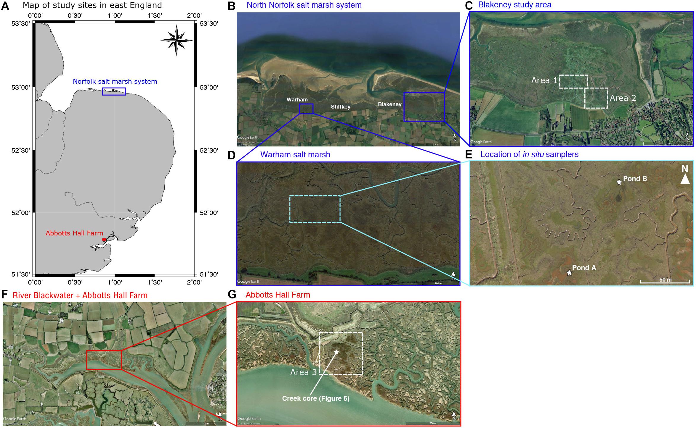
Figure 1. (A) Map of east England showing the Norfolk salt marsh system and Abbotts Hall Farm nature reserve (Essex wildlife trust). Scale from latitude/longitude lines. (B) Google Earth satellite imagery (24-09-17) of the Norfolk salt marsh system comprising Warham marshes, Stiffkey marshes and Blakeney marshes (labeled). Cores in the data compilation were taken throughout this area. The blue box denotes the location of (D). Image credit: Google Earth, Image 2018 DigitalGlobe (C) Google Earth Satellite imagery (31-12-1999) of Blakeney salt marsh. Area 1 and 2 correspond to the mapped areas in Figures 7 and 8 respectively. (D) Google Earth satellite imagery (10-01-2019) of the Warham salt marsh area where in situ samplers are installed. Light blue box indicates location of (E). Image credit: Google Earth. (E) Location of in situ samplers (Pond A and B) in Warham salt marsh. (F) Google Earth satellite imagery (06-11-2006) of the River Blackwater and the location of Abbotts Hall Farm nature reserve. Red box denotes the location of (G). Image credit: Google Earth, 2018 Infoterra Ltd & Bluesky. (G) Google Earth satellite imagery (06-11-1999) of Abbotts Hall Farm salt marsh system. Area 3 corresponds to mapped area in Figure 9. White star denotes location of core taken in Figure 5. Image credit: Google Earth, 2018 Infoterra Ltd & Bluesky.

We describe the geochemical nature of these pond sediments using multiple push cores taken over a 5-year period and an in situ sampler from which samples were collected over the course of 1 year. A drone survey was carried out to map the distributions of the types of ponds to understand the mechanisms governing the pond sediment geochemistry. We offer potential hypotheses and areas of investigation for the observed spatial and temporal geochemical patterns. We test the distribution of overlying water depth on the pond sediment, the distribution of carbon within surface sediments and we look for evidence of groundwater fluxes in the salt marsh sediment for preliminary insights into the system.

Materials and Methods

Field Locations

This study discusses fieldwork undertaken in salt marsh systems across East Anglia, both in Norfolk, United Kingdom and at Abbotts Hall Farm, Essex, United Kingdom (Figure 1). On the Norfolk coastline, protection offered by migrating barrier islands, spits and intertidal sand flats have allowed salt marsh systems to form since the start of the Holocene (Pethick, 1980). In Norfolk, our field locations are three developed areas of stable, upper salt marsh near the small towns of Blakeney, Warham, and Stiffkey (Figure 1B). Areas 1 and 2 for the drone mapping are locations in the Blakeney salt marsh area (Figure 1C). In these sites, the lower marsh is more recent (post-medieval) whereas the upper, stable, marsh is Romano-British (2000+ years) (Pethick, 1980). The upper marsh sediment consists of grayish-brown, silty sands and clayey silts, likely accumulated by vegetative capture of finer grained sediment, which sits upon a northward dipping boulder clay (Pye et al., 1990). Abbotts Hall Farm is a nature reserve on an estuarine portion of the River Blackwater (Figure 1F). Area 3 (Figure 1G) lies on the edge of this tributary (defined as fringed-estuarine) where low energy environments are protected from direct wave action (Allen, 2000). Sediment in this location was previously not well studied; we observe it to be similar to that in the Norfolk marshes, likely reflecting similar provenance of sediment.

Porewater Collection

Push core liners made of polyvinyl chloride (PVC) were used to extract vertical columns of sediment from ponds at irregular intervals over the period 2013–2018. One core, taken in May 2018, was pushed horizontally into the side of a creek at 20 cm depth. Porewater was extracted from the cores either in the field or within 24 h of being collected using Rhizons (syringe-based samplers with an inert polymer membrane). Samples for each core were taken at variable depth resolutions (between 1 and 4 cm; see data table in Supplementary Information). Typically, between 2 and 10 mL of porewater was extracted from each depth sampled, depending on the sediment porosity and what was needed for analysis. Aliquots of porewater (50–2000 μL) for ferrous iron analysis were fixed with 100 μL ferrozine reagent; the precise amount of porewater depended on the amount of iron present. Aliquots (50–2000 μL) for aqueous sulfide were fixed with excess quantities—dependent on sulfide concentration—of either 5 or 20% zinc acetate.

Analytical Measurements

All analytical measurements were carried out at the University of Cambridge. Dissolved iron concentrations [Fe(II)] were determined spectrophotometrically (Thermo Aquamate UV-Vis) according to the method described by Stookey (1970) with an error of 0.4%. Dissolved sulfide concentrations were measured spectrophotometrically using the methylene blue method with an error of 2% and a detection limit of 1 μM (Cline, 1969). Samples were diluted with ultrapure water to fit within a calibrated range. Major anion (sulfate and chloride) concentrations were measured by ion chromatography (Thermo Scientific Dionex ICS5000+) with an error up to 2% based on repeat analysis of standards. Samples measured for alkalinity were filtered using a cellulose nitrate membrane syringe filter (0.2 μM, 47 mm). Alkalinity was determined using the inflection point method by titrating 1–1.2 mL aliquots of filtered samples with 0.0166 M analytical grade hydrochloric acid (HCl). The pH was measured at 25°C on the NBS scale using an Orion 3 Star meter with a ROSS micro-electrode (ORION 8220 BNWP PerpHect ROSS).

Samples for sulfur isotope analysis were separated into vials and a supersaturated barium chloride solution was added, precipitating barite (BaSO₄). The barite was cleaned using 10% HCl, triple washed with ultrapure water, and dried. The δ³⁴S_SO4 was determined through combustion on a Flash Element Analyzer (Thermo Scientific) coupled with continuous helium flow to a Delta V Plus mass spectrometer. Samples were corrected to NBS-127 barite standards (δ³⁴S = 20.3‰) which were run before and after sets of 20 samples. Based on blind replicates and repeat running of the standard, the data had precision of 0.2‰ (1σ). Sulfur isotopic compositions are reported in standard delta notation as per mil (‰) deviations from the Vienna Cañon Diablo Troilite (VCDT).

Mapping of Ponds

We used a drone (Phantom 3 Standard) to create an aerial survey at a height of 150 m in May 2018. The orthophotos were assembled using the MapsMadeEasy website and the projection used for uploading to QGIS was WGS 84 31N. We were unable to drone map Area 3, in Abbotts Hall, so we used Google Earth satellite imagery of the area. Two ground-truth campaigns—in May and July 2018—were undertaken to characterize pond sediment types from the drone images. Using the different surface characteristics typical of an iron-rich pond and a sulfide-rich pond (described in results), we were able to classify 350 ponds using the flowchart presented in Figure 2 (see Supplementary Table S1 and Supplementary Figures S1–S5 for full observed attributes and methods of characterization). For each pond visible in the aerial images, we would classify it as an iron-rich pond sediment, a sulfide-rich pond sediment or as ‘intermediate’ between iron-rich and sulfide-rich. The third category was necessary given that some ponds contained attributes of both iron- and sulfide-rich sediments. We attempted to characterize ponds directly from the drone imagery but this proved impossible given the variable surface colors and the small scale of the distinguishing features. At each pond, we measured the depth of the overlying water column using a tape measure. We also recorded the following characteristics for 267 of the 350 ponds for statistical analysis: the presence of algae (Supplementary Figure S5), signs of bioturbation (worm casts) (Supplementary Figures S1, S2), the presence of sulfur oxidizing bacteria (Beggiatoaceae) (Supplementary Figure S3) and signs of desiccation cracks (Supplementary Figure S6).

FIGURE 2

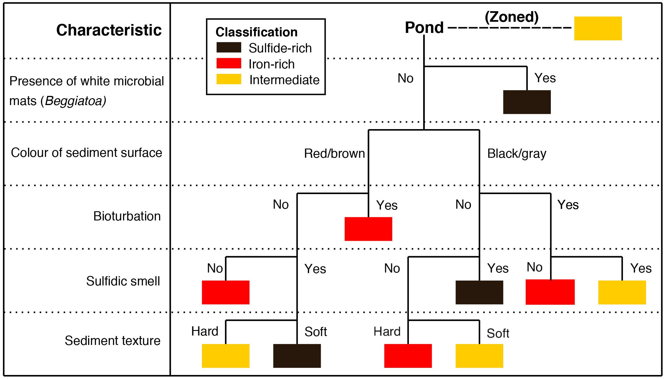
Figure 2. Typical method of characterization of an individual pond based on features visible and/or easily testable from the surface. Flowchart is constructed in order of most diagnostic and most easily characterized (e.g., the presence of Beggiatoaceae and surface color are far quicker to differentiate than the sediment texture). The presence of white microbial mats, presumed to be Beggiatoaceae and resulting oxidized sulfur products present on the sediment surface, was decided to be sufficient enough evidence that sulfate reducing conditions were present in these ponds (Supplementary Figure S3). The color of the sediment surface was typically well differentiated; ponds were either a very dark gray color or had a red/brown tint to them (similar to iron oxide coloration). If the pond sediment surface was a different color to this or was a shade between the classifications, this category would be ignored for the classification. The presence of bioturbation was ascertained by worm casts seen on the sediment surface (Supplementary Figures S1, S2 for evidence). The presence of a single worm cast was deemed sufficient to assign a positive result to this category. The sulfidic smell property relates to a strong sulfidic odor when the sediment was removed from the water and handled. Sediment texture was determined by handling of the top 5 cm of sediment. When touched, certain sediments were clearly very soft and fluffy at the surface, whilst others had a stiffer clay texture. These would be defined as soft and hard respectively. Some characteristics were occasionally present but in spatially isolated zones on the pond (e.g., signs of bioturbation on one side of the pond and white microbial mats on the other). This is defined as ‘zoned’ on the diagram and ponds of this nature were classified as intermediate. This method is preferred to geochemical analysis as it is quicker than sampling and allows for rapid characterization of the salt marsh system.

In situ Sampling

In order to monitor geochemical changes in individual pond sediments over time, in situ samplers were designed to allow repeated sampling of pond sediment pore fluids without disturbing the sediment. The submerged samplers consist of plastic frames to which Rhizon filters are attached at 2 cm intervals starting from the sediment-water interface to a depth of 34 cm (see Supplementary Figure S7 for construction). Outlets from the Rhizons were connected to sampling ports via airtight, double-walled, (<60 cm) tubes (polyethylene inner and polyvinylchloride outer, ID = 1mm) to the surface to which 10 mL syringes were attached for extraction. We selected spacing of 2 cm so that sampling volume from separate Rhizons remains discrete and does not result in artificial drawdown of surface water, based on tracer and modeling studies (Seeberg-Elverfeldt et al., 2005).

In situ samplers were installed in two Warham salt marsh ponds (termed Pond A and Pond B) in January 2017 (Figures 1D,E). Pond A appeared to contain sulfide-rich pond sediment—using the above criteria—whilst the other, Pond B, an elongate pond in shape, was defined as intermediate. Samples of pore fluids from sediment in both ponds were collected in March, April, May, July, and November 2017, and May 2018. During each sampling, the stagnant fluid in the tubing (roughly 0.6 mL for 60 cm of 1 mm ID tubing) was first removed by extracting and discarding 1–2 mL of pore fluid from each outlet. Another 4–5 mL of pore fluid was then extracted for geochemical analysis. All depths were sampled simultaneously.

Carbon Content Analysis

In May 2018, sediment was taken from the surface of 30 ponds in Abbotts Hall (Area 3 on Figure 1G) using a 1 mL syringe with a cut edge. Sediments were dried and analyzed for total carbon content using a Costech element analyzer coupled via continuous flow to a Delta V mass spectrometer. Five samples were tested for the presence of carbonate minerals using a duplicate washed in 0.1 M HCl and subsequently triple washed with ultrapure water. As there were no carbonate minerals found, total carbon content is assumed to come from the organic carbon fraction.

Results

Sediment Cores Taken Over the 2013–2018 Period

The subsurface geochemistry of ponds in the East Anglian salt marshes is reflected in characteristics observed at the sediment surface; iron-rich pond sediments are often stained red at the surface, contain worm casts and iron-oxide films are occasionally visible on the water surface; whereas sulfide-rich pond sediments are typically gray/black, commonly contain sulfide oxidizing bacteria on the sediment surface (Beggiatoaceae) and exude a strong sulfidic odor. Sulfide-rich pond sediments have a higher porewater methane concentration, in contrast, iron-rich pond sediments have no methane present (Mills et al., 2016).

Figure 3 shows porewater data collected from two cores; an iron-rich core taken from Stiffkey, August 2015, and a sulfide-rich core taken from Blakeney, August 2015. We note the key features of iron-rich versus sulfide-rich pond sediment porewater in Figure 3. In the iron-rich sediment there are high concentrations of ferrous iron, little change in the δ³⁴S_SO4, near-zero aqueous sulfide, near seawater [SO₄]/[Cl] ratios, lower overall pH and low alkalinity (Figure 3, red). In contrast, in the sulfide-rich pond sediment there is no measurable ferrous iron, an increase in δ³⁴S_SO4 by 40‰, sulfide concentrations above 4 mM, lower [SO₄]/[Cl] ratios relative to seawater, higher pH and higher pore fluid alkalinity (Figure 3, black). The concentration of both chloride and sulfate in the overlying pond water are lower than typical seawater. In particular, the surface 20 cm of the iron-rich pond contains very low porewater chloride concentrations (200–400 mM, 30–60% lower than seawater) (Figures 3E,F). We present these cores, collected in August 2015, separately (Figure 3) as they were the only two cores on which pH and alkalinity were measured in addition to other geochemical parameters. Figure 4 presents a more limited geochemical dataset collected from far more cores taken over the three field sites shown in Figure 1B between 2013 and 2017. Cores taken through the vegetated platform surrounding these ponds are included (denoted as ‘vegetated’) for an understanding of the porewater profiles in the rest of the marsh where there is an absence of ponds. In one case, we took multiple cores from the same sulfide-rich pond and found near identical geochemistry across the pond (Supplementary Figure S8), thus we conclude each core accurately represents the geochemistry of the whole pond from which it was sampled.

FIGURE 3

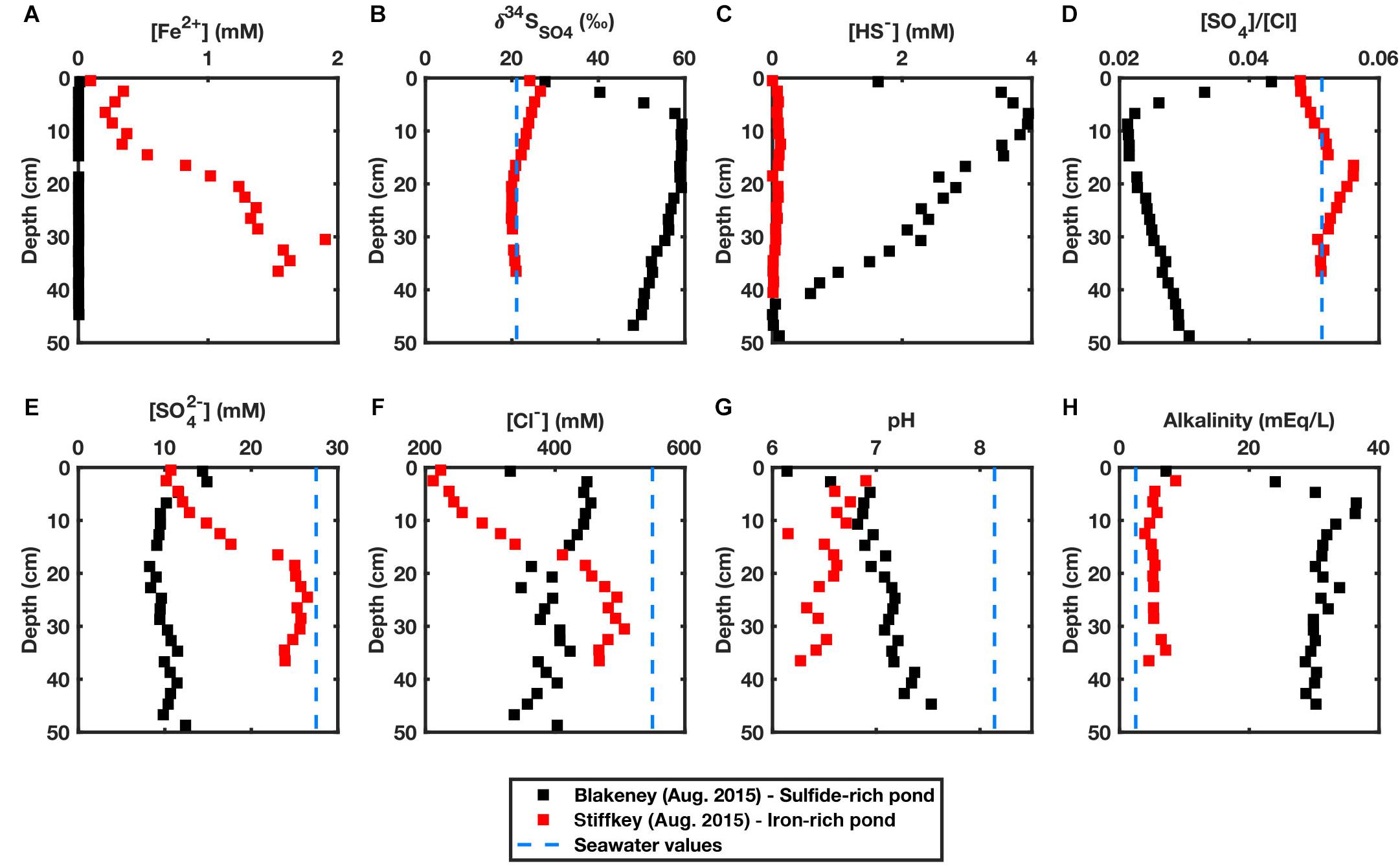
Figure 3. Geochemical characteristics of porewater extracted from an iron-rich core from Stiffkey in August 2015 (shown in red) and a sulfide-rich core from Blakeney in August 2015 (shown in black). (A) Aqueous Fe(II) concentrations (mM) (B) δ³⁴S_SO4 (‰) (C) Aqueous sulfide concentrations (mM) (D) [SO₄]/[Cl] ratio (E) Aqueous sulfate concentrations (mM) (F) Aqueous chloride concentrations (mM) (G) pH values (H) Alkalinity (mEq/L). Dashed blue lines represent typical seawater values (seawater concentrations of Fe²⁺ and HS^- are negligible).

FIGURE 4

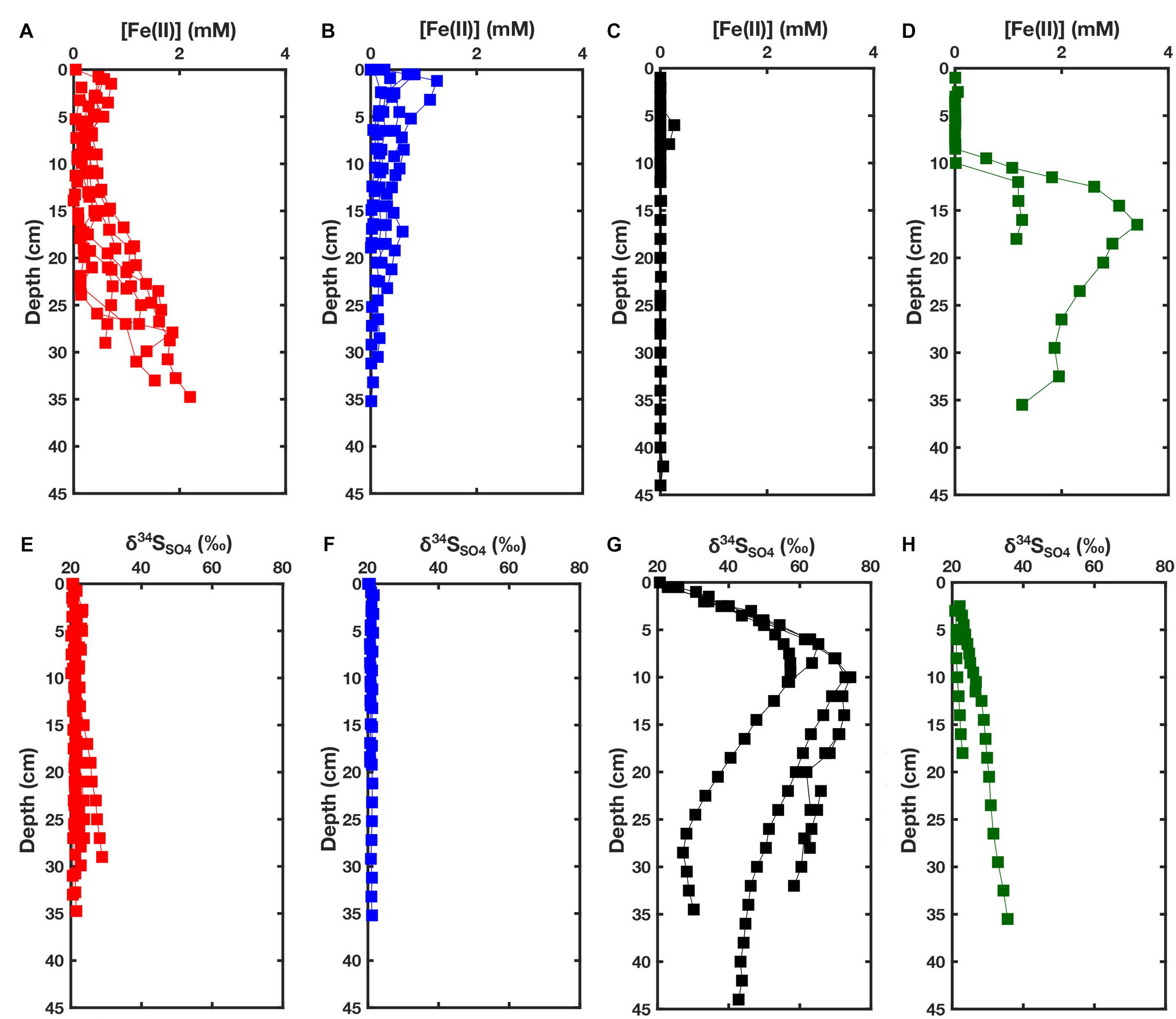
Figure 4. (A) Fe(II) concentrations in iron-rich pond sediment porewaters, with increasing Fe(II) with depth, sampled in November 2013 (Warham), November 2013 (Stiffkey), January 2014 (Warham), May 2014 (Warham), October 2015 (Antler et al., unpublished), October 2015 (Stiffkey) and October 2017 (Blakeney). (B) Fe(II) concentrations in iron-rich sediment porewaters, with decreasing Fe(II) with depth, sampled in November 2013 (Stiffkey), November 2013 (Stiffkey), March 2014 (Warham), December 2017 (Blakeney) and December 2017 (Blakeney). (C) Fe(II) concentrations in sulfide-rich pond sediment porewaters. Only three cores [October 2015 (Antler et al., unpublished), October 2015 (Blakeney) and December 2017 (Blakeney)] are presented here since Fe(II) concentrations are typically below detection limit using our analytical method. (D) Fe(II) concentrations in sediment porewaters in cores taken from the vegetated platform in November 2013 (Warham) and October 2015 (Warham). (E) δ³⁴S_SO4 profiles in iron-rich pond sediment porewaters sampled in November 2013 (Warham), November 2013 (Stiffkey), January 2014 (Warham), May 2014 (Warham), October 2015 (Antler et al., unpublished) and October 2015 (Stiffkey) (Note: Not all cores present in subplot A are present here). (F) δ³⁴S_SO4 profiles in iron-rich pond sediment porewaters sampled in November 2013 (Stiffkey), November 2013 (Stiffkey) and March 2014 (Warham) (Note: Not all cores present in subplot B are present here). (G) δ³⁴S_SO4 profiles taken from sulfide-rich cores sampled in November 2013 (Blakeney), November 2013 (Blakeney), November 2013 (Blakeney), October 2015 (Antler et al., unpublished) and October 2015 (Blakeney). (H) δ³⁴S_SO4 profiles from cores taken from vegetated platforms in November 2013 (Warham) and October 2015 (Warham). Vegetated cores are taken from the sediment surface whereas iron-rich and sulfide-rich pond cores have an undefined column of water on the surface.

Dissolved ferrous iron (Fe²⁺) concentrations of porewater in our compilation of cores indicate that there are two broad types of pond sediments (Figures 3A, 4A,B). Ferrous iron in iron-rich sediment porewater is present at millimolar concentrations, whereas concentrations are below the detection limit (3 μM) in sulfide-rich sediment porewater (Figures 3A, 4C). We find, however, that there are variations in the general pattern of ferrous iron concentrations within pond sediments broadly classified as ‘iron-rich.’ In some cores, porewater ferrous iron concentrations increase with depth, sometimes reaching as high as 2 mM at 35 cm depth (Figure 4A). In these cores, lower ferrous iron concentrations are observed from 5 to 15 cm, but iron and manganese oxides are visible, giving the sediments an orange hue in the core within this depth range. Conversely, in the other subset of ‘iron-rich cores’ there is a decrease in ferrous iron concentration with depth (Figure 4B). Ferrous iron concentrations in cores taken from the vegetated platform in Warham are near zero up to 8–10 cm from the surface (this coincides with the depth of root penetration) (Figure 4D). Below this rooting zone, porewater ferrous iron concentrations increase up to 3 mM—the highest observed in any of the cores.

Both types of iron-rich core have similar porewater δ³⁴S_SO4, either a minor increase with depth or a constant δ³⁴S_SO4 near that of seawater (Figures 3B, 4E,F). In sulfide-rich cores (Figures 3B, 4C,G), δ³⁴S_SO4 increases up to 70‰ by 15–25 cm depth below the sediment-water interface. This is coincident with an increase in sulfide concentrations and decrease in sulfate concentrations (Figures 3C,D). In vegetated cores (Figure 4H), there is an increase of approximately 5–15‰ in δ³⁴S_SO4 from 0 to 35 cm.

It should be noted that absolute depths cannot be accurately compared among the sampled ponds because water depth was not always recorded in ponds where sediment cores were taken and we do not have elevation data for the salt marsh platforms. For the full compilation of geochemical data acquired on cores from 2013 to 2018, see the Supplementary Material.

In the core extracted from the creek wall edge, all geochemical measurements show large changes within 5 cm from the creek-sediment boundary (Figure 5). In this zone, a threefold decrease in iron concentration is observed toward the creek edge. This is accompanied by higher concentrations of chlorine and sulfate and lower δ³⁴S_SO4. From 5 cm inward, the geochemistry is much more stable. Ferrous iron concentrations are significantly higher (6 mM) than those seen in the other cores taken.

FIGURE 5

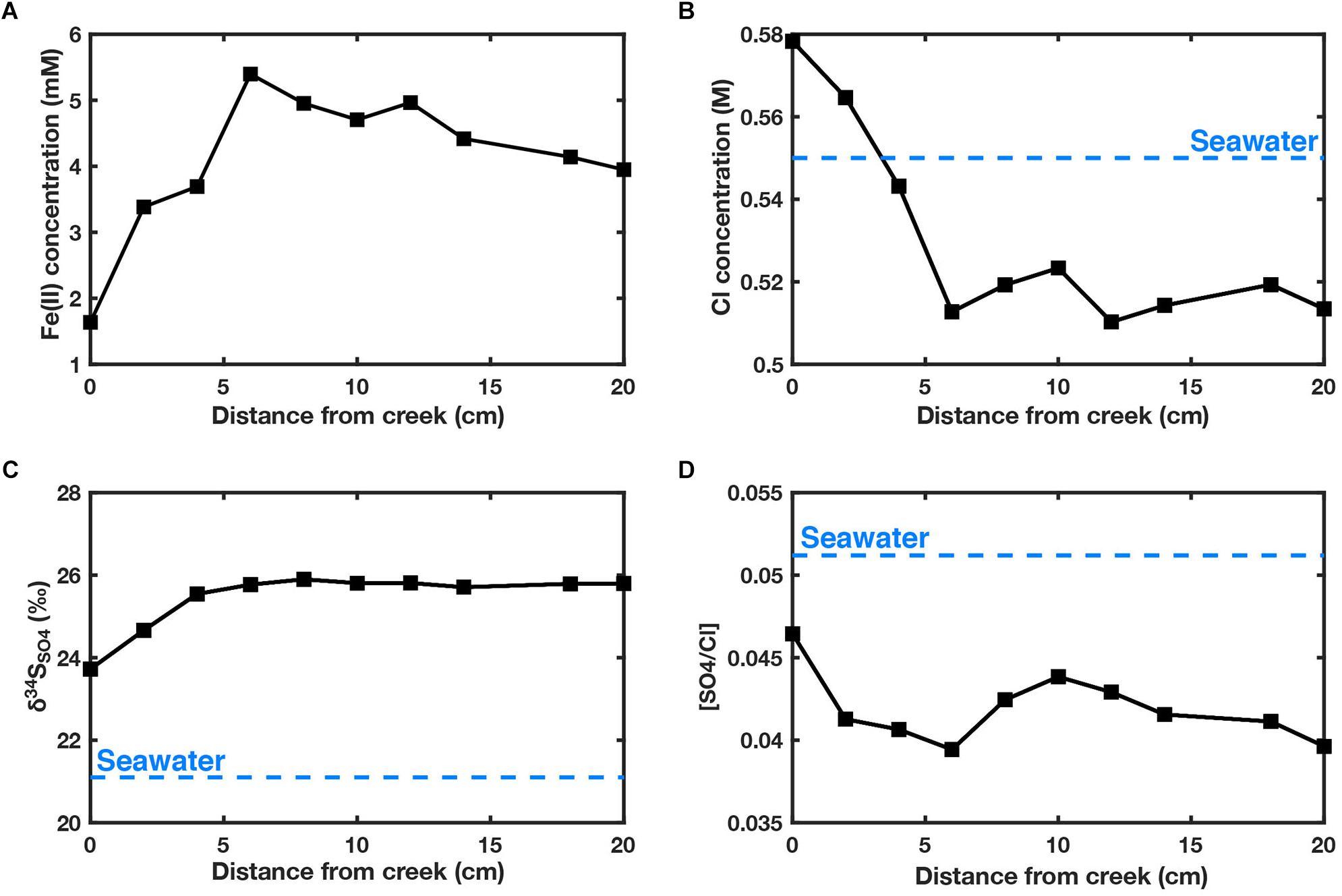
Figure 5. Core horizontally extracted from creek wall (see Figure 1 for location). Depth is 20 cm from the surface of the salt marsh. (A) Fe(II) concentrations (mM) (B) Cl concentrations (M) (C) δ³⁴S_SO4 (D) [SO₄]/[Cl]. Blue dashed line corresponds with seawater values. Location shown in Figure 1.

In situ Sampling From March 2017 – May 2018

Two ponds were sampled using in situ samplers over the year from March 2017 - May 2018. Pond A (sulfide-rich pond) shows small seasonal variations in δ³⁴S_SO4 of porewater sulfate with higher δ³⁴S_SO4 observed in the summer and autumn months (Figure 6A). These variations are more pronounced in the upper 15 cm and values become more uniform (within 10‰) below this. Changes in δ³⁴S_SO4 in Pond B (an intermediate pond) are far greater (Figure 6B); in March 2017, the δ³⁴S_SO4 is constant with depth and only slightly elevated from the values seen in a ‘typical’ iron-rich pond. Ferrous iron concentrations were negligible in both ponds for months March-July and aqueous sulfide is present in both ponds in May 2018, albeit it at higher concentrations in Pond A (Supplementary Figure S9).

FIGURE 6

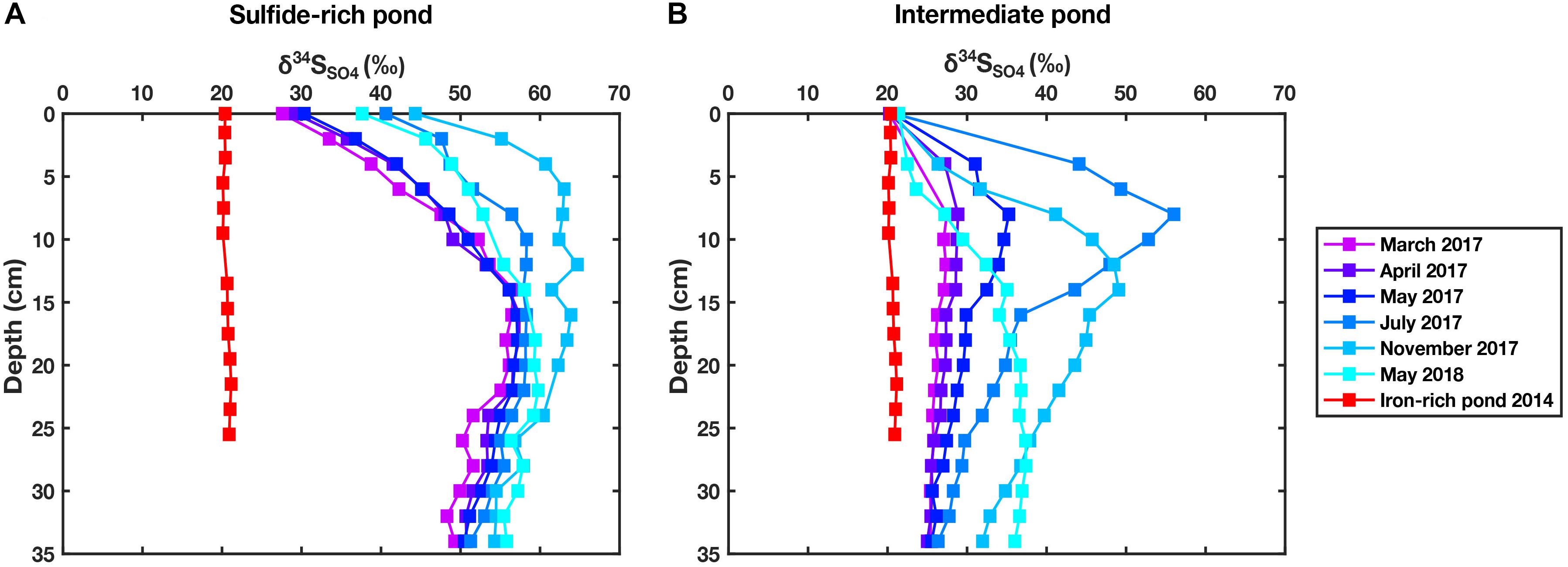
Figure 6. (A) δ³⁴S_SO4 measured in porewater samples over a 14-month period for pond A (sulfide-rich pond). Data from an iron-rich pond sampled in 2014 is added for comparison. Analytical uncertainty is 0.2‰. (B) δ³⁴S_SO4 measured in porewaters over a 14-month period for pond B (intermediate pond). Data from an iron-rich pond from 2014 is added for comparison. Analytical uncertainty is 0.2‰.

Whilst the pond sediment appears to become more sulfide-rich with time, there is a decoupling between the shallow (<20 cm) and the deep zone (>20 cm). The shallow zone displays greatest ³⁴S enrichment - δ³⁴S_SO4 up to 55‰—during July 2017 before falling to lower δ³⁴S_SO4 in November 2017 and May 2018. In contrast, the deep zone shows a consistent increase in δ³⁴S_SO4 through time—up to 35‰ in May 2018.

Mapping of Pond Distributions

Two areas from the Blakeney salt marsh system were mapped using an aerial drone survey and an area in the Abbotts Hall salt marsh system (Figures 1F,G) was mapped using Google Earth satellite imagery (Figures 7–9). Area 1, from Blakeney (Figure 7) consists of two groups of ponds separated by a tidal creek. Ponds containing sulfide-rich sediment tend to be situated further from large creek networks than ponds containing iron-rich sediment (Figure 7B). The presence of sulfide-rich ponds is often accompanied by a region of standing water on the surrounding vegetated platform (visible in Figure 7A). Ponds of a similar geochemical and geomorphological nature appear to cluster in groups. Intermediate ponds, displaying neither or both criteria for iron-rich or sulfide-rich ponds, often lie at the boundary between iron-rich and sulfide-rich pond clusters. There are also clear differences in the vegetation over the marsh. The center of the platform is characterized by salt marsh ‘lawn’ species (typically some combination of Puccinellia spp., Salicornia spp., and Sesuvium portulacastrum) whereas the areas closest to the creek have larger species (Atriplex spp. and Suaeda spp.).

FIGURE 7

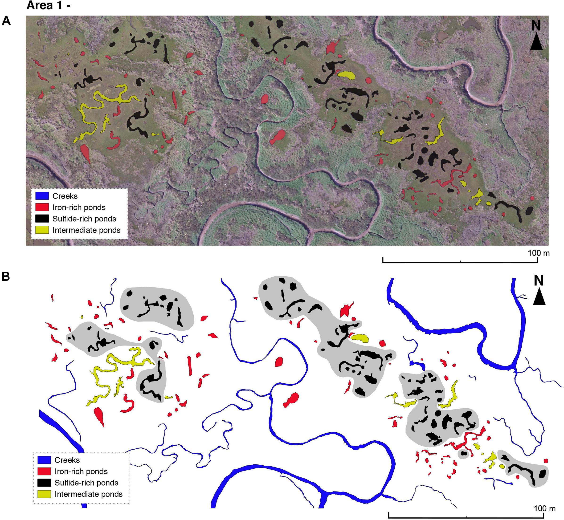
Figure 7. (A) Drone imagery taken on 03/05/18 of two aggregates in Blakeney salt marsh area 1 (see Figure 1C) overlain by geochemical classification observed over the period from May and July 2018. We changed the classification of only two ponds between May and July 2018—both were changed from sulfide-rich to intermediate. (B) Geochemical classification of ponds sediments. Hypothetical, hand-drawn zones of sulfide-rich pond clustering shown in gray.

In an area of upper marsh (the oldest, most inland marsh) (Figure 1C), ponds with sulfide-rich sediment concentrate at the point furthest inland and iron-rich or intermediate ponds are located more toward the littoral zone (Figure 8). Drone imagery shows vegetation debris on the vegetated platform with sulfide-rich ponds (south of Figure 8A) and larger vegetation (likely Spartina patens) around the edges of sulfide-rich ponds (seen as gray patches surrounding ponds in south of Figure 8A). Proximity to larger creeks appears to favor the presence of ponds with iron-rich sediment (north in Figure 8A).

FIGURE 8

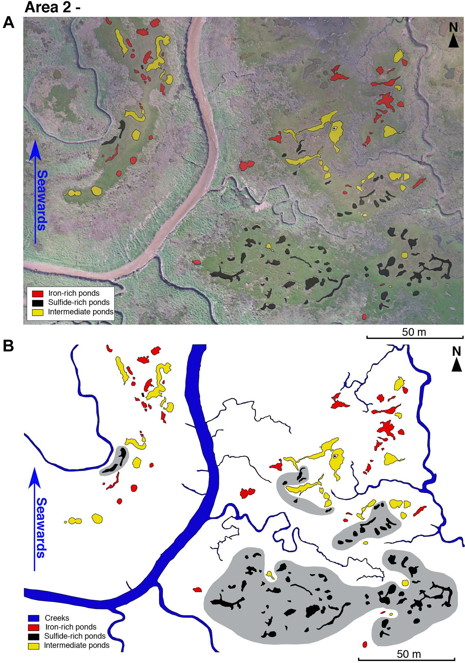
Figure 8. (A) Drone imagery taken on 03/05/18 of an aggregate in Blakeney salt marsh area 2 (see Figure 1C) overlain by geochemical classification observed over period from May 2018. (B) Geochemical classification with hypothetical, hand-drawn zones of sulfide-rich pond clustering shown in gray.

At Abbotts Hall, we observe a similar pattern of internal salt marsh ponds being more sulfide-rich (Figure 9B), albeit with more exceptions than in Areas 1 and 2 (from Norfolk). Iron-rich vs. sulfide-rich pond sediment distribution does not seem to correlate with the type of vegetation observed on satellite imagery (Figure 9A). An artificial drainage ditch (north east of area) is proximal to an area of what we have defined as ‘intermediate ponds.’

FIGURE 9

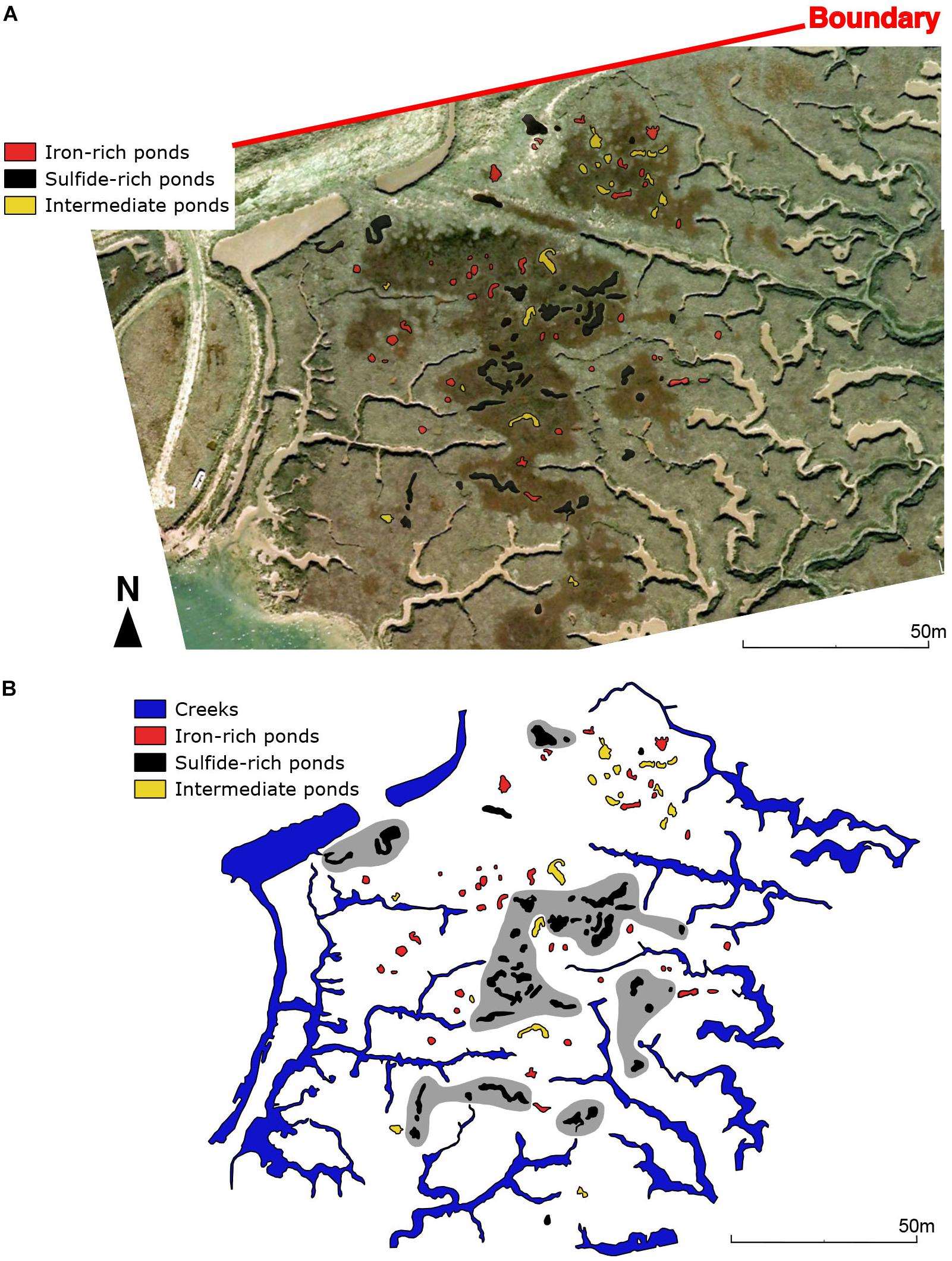
Figure 9. (A) Google Earth imagery (06/11/2006) of the salt marsh system in Abbotts Hall (Area 3) (Figure 1G) overlain by geochemical classification observed in June 2018. (B) Geochemical classification with hypothetical, hand-drawn zones of sulfide-rich pond clustering shown in gray. Boundary depicted on panel (A) corresponds to landward extent of the salt marsh.

Pond Characteristics and Water Depths

There is a correlation between water depth and the type of pond sediment geochemistry; the average pond water depth in sulfidic pond sediments is deeper than that of iron-rich pond sediments [Area 1—mean iron-rich pond water depth = 20.2 ± 5.0 cm (n = 60), mean sulfide-rich pond water depth = 24.1 ± 4.7 cm (n = 50) (two sample t-test, p < 0.05); Area 2—mean iron-rich pond water depth = 19.1 ± 5.6 cm (n = 40), mean sulfide-rich pond water = 22.4 ± 5.5 cm (n = 64) (two sample t-test, p < 0.05); Area 3—mean iron-rich pond water depth = 11.8 ± 4.0 cm (n = 40), mean sulfide-rich pond water depth = 15.2 ± 4.6 cm (n = 40) (two sample t-test, p < 0.05) (Figures 10B–E)].

FIGURE 10

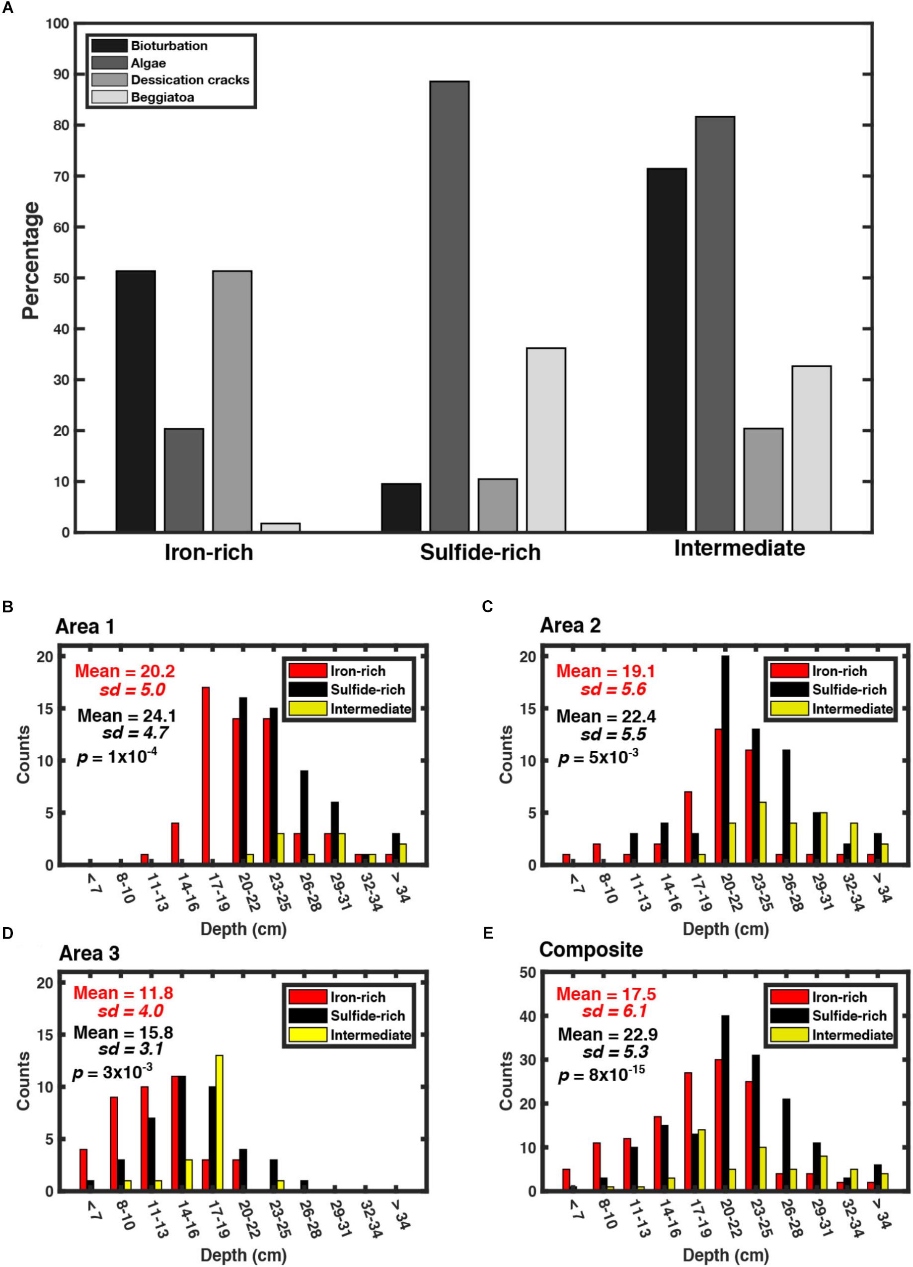
Figure 10. (A) Characteristics [bioturbation, algae, desiccation cracks and sulfide oxidizing bacteria (e.g., Beggiatoaceae)] observed in each category of pond taken in the three areas. (B) Water depth measurements taken in Area 1 for each type of pond (17/05/18). P-value taken from t-tests testing the null hypothesis that there is no difference in water depth between pond classfications. (C) Water depth measurements taken in Area 2 for each type of pond (17/05/18). (D) Water depth measurements taken in Area 3 for each type of pond (19/06/18). (E) Composite made of all depth measurements taken from Area’s 1, 2, and 3.

After identifying the presence of certain features notable from the pond surface, (bioturbation evidence, presence of algae in the surface water, presence of Beggiatoaceae and the presence of desiccation cracks) we observe that cracks, evidence of a transient drying effect, are less prevalent in sulfide-rich ponds compared to iron-rich ponds and intermediate ponds (Figure 10A). This is consistent with the observation that sulfide-rich ponds in general have greater water depths and thus dry out less frequently (Figure 10E). Conversely, the presence of algae is common in sulfide-rich (90%) and intermediate ponds (80%) and yet is only present in 30% of iron-rich ponds. Since we used both the presence of white microbial mats (Beggiatoaceae) and bioturbation as tools for characterizing ponds, it is unsurprising that we find bioturbation to be common in iron-rich ponds and sulfide oxidizing bacteria to be negligible. Intermediate ponds contain any combination of characteristics; in particular, the presence of both algae and bioturbation was common (>70%).

Discussion

Salt Marsh Pond Geochemistry

In the absence of microbial data on the pond sediments, we use the porewater geochemistry, that is the concentrations of various redox-sensitive species, to infer the biogeochemical processes occurring within the sedimentary environment. For example, the presence of ferrous iron [Fe(II)] suggests that reduction of ferric iron is occurring, either through bacterial iron reduction (Equation 1) or the reduction of ferric iron coupled to sulfide oxidation (Equation 2). Similarly, the presence of aqueous sulfide would suggest the presence of either microbial sulfate reduction (Equation 3) or dissolution of sulfide-containing minerals in the environment. The δ³⁴S_SO4 of the porewater sulfate allows us to identify the occurrence of microbial sulfate reduction because during microbial sulfate reduction, bacteria preferentially utilize sulfate with the lighter ³²S isotope over the heavier ³⁴S isotope. This leads an isotopically lower sulfide pool and a residual porewater sulfate pool enriched in the heavier isotope; the opposite would be true if there were dissolution of sulfide minerals. In this way we use the geochemistry that we have measured to infer the microbially driven processes that are occurring in the salt marsh sediment.

$4Fe{(OH)}_3+7H^{+}+C{H}_{2}O\to HC{O}_3^{-}+4F{e}^{2+}+10H_{2}O$ (1)

$H{S}^{-}+2Fe{(OH)}_3+5H^{+}\to 2F{e}^{2+}+S^{\circ }+6H_{2}O$ (2)

$2C{H}_{2}O+S{O}_4^{2-}\to H_{2}S+2HC{O}_3^{-}$ (3)

Our data, along with pH and alkalinity, demonstrate that there are two broad classifications of pond sediment in the studied East Anglian salt marshes. Some pond sediments contain porewater with high δ³⁴S_SO4, high quantities of aqueous sulfide and declining SO₄/Cl ratios indicative of sulfate consumption; these pond sediments are interpreted to sustain high levels of microbial sulfate reduction. The other group of pond sediments contain porewater with near seawater δ³⁴S_SO4, seawater SO₄/Cl and high quantities of ferrous iron. These ponds are likely dominated by bacterial iron reduction, potentially in addition to a cryptic sulfur cycle in which reduced sulfur species are nearly quantitatively recycled back to sulfate (Mills et al., 2016). These pond sediments are referred to as sulfide-rich and iron-rich, respectively.

This broad dichotomy arises due to the titration reaction between sulfide and ferrous iron or iron monosulfides (Equations 4 and 5) which means only one of the species (the one in excess) can be present in significant quantities (Drobner et al., 1990). The pond sediment ‘type’ therefore reflects environmental conditions which favor production of either reduced iron or aqueous sulfide. The aim of this study is to understand why such contrasting sediment redox states can be seen separated by less than five meters and yet two sulfide-rich ponds, for example, can be almost identical across hundreds of kilometers over East Anglia.

$F{e}^{2+}+H{S}^{-}\to FeS+H^{+}$ (4)

$FeS+H_{2}S\to Fe{S}_2+H_2$ (5)

The conditions which favor certain microbial metabolisms are complex. In contrast to the canonical view of the redox ladder (Froelich et al., 1979), when pH is circumneutral there is a convergence of the useable energies for iron reducing bacteria, sulfate reducing bacteria, and even methanogenic bacteria (Bethke et al., 2011). Furthermore, multiple studies have seen interplay among redox cycles (Mortimer et al., 2011; Hansel et al., 2015; Antler et al., unpublished).

We find evidence of this interplay; despite changes in alkalinity that are more consistent with iron reduction or sulfate reduction dominating a sediment, the fact that pH decreases with depth in the iron-rich core (Figure 4E) is counter-intuitive because bacterial iron reduction consumes protons and thus raises pH (Soetaert et al., 2007). We suggest other redox reactions are working in tandem with bacterial iron reduction, causing the decrease in pH. One example could be Equation (4) or the regeneration of ferric iron (Soetaert et al., 2007). The net result of the reactions present are not well understood currently, and characterization of the fundamental chemical reactions involved is necessary to understand changes in sedimentary pH. This complexity and closeness of energies among metabolisms means even subtle differences in the speciation and quantity of the electron acceptor; the speciation and quantity of the electron donor; and the influence of other redox cycles within the sediment could alter which metabolism, and therefore which geochemistry, dominates.

One observable difference is that 50% of iron-rich ponds contain evidence of bioturbation on the sediment surface (Supplementary Figures S1, S2), a result of species such as polychaete worms (Nereis spp.) and lugworm (Arenicola spp.) burrowing between 5 and 15 cm depth (Antler et al., unpublished). The amount of worm casts in iron-rich ponds and worm density in sediment varies substantially, although the 5–15 cm depth increment contains the highest density of worms (Antler et al., unpublished). This process would introduce pathways for oxic waters into an otherwise diffusion-dominated, anoxic system, potentially providing redox conditions which could regenerate ferric phase minerals [likely poorly ordered iron (oxyhydr)oxides] which become available for further bacterial iron reduction. Although sulfide produced through microbial sulfate reduction, thought to be active in iron-rich sediments due to the presence of reduced sulfide minerals, could titrate some of this iron away (Antler et al., unpublished), the ongoing regeneration of Fe(III) phases creates favorable conditions for iron reduction over other microbial metabolisms, resulting in high ferrous iron concentrations within the sedimentary porewater. Conversely, in sulfide-rich pond sediment, no worm casts are seen, implying there is no bioturbation. This is likely due to the build-up of aqueous sulfide, generating toxic conditions which preclude the presence of bioturbating organisms. A lack of bioturbation limits mixing of the surface sediment, and hence oxygen penetration within the system. This leads to a positive feedback mechanism where ferrous iron would react with sulfide instead of being regenerated into ferric iron phases. Microbial sulfate reduction would become the dominant reduction pathway, using seawater sulfate as the electron acceptor.

Within the broad categories of iron-rich and sulfide-rich sediment, we find pond sediment chemistry can vary in terms of absolute concentrations of either iron or sulfide. All iron-rich cores have a depletion in ferrous iron concentrations from 5 to 15 cm; as suggested above, bioturbation in this region introduces oxygen to the system and reoxidises most aqueous Fe(II). However, beneath this zone, ferrous iron concentrations in porewaters can either increase from 15 to 35 cm in some cores (Figure 4A) or continue to decrease to negligible concentrations below 15 cm (Figure 4B). No major difference is observed in the corresponding δ³⁴S_SO4 (Figures 4E,F). This discrepancy among profiles of ferrous iron could be due to different iron minerals present at depth, though it is not intuitive why there would be significant differences in mineralogy or concentration of iron minerals over a salt marsh platform. Another potential reason for the increase in Fe(II) is reduction of Fe(III), coupled to deep sulfide oxidation in some cores (Mortimer et al., 2011; Hansel et al., 2015). This would be undetectable in sulfide or sulfate concentrations or δ³⁴S_SO4 if it were near quantitative, implying some kind of ‘cryptic’ sulfur cycling was occurring (Holmkvist et al., 2011; Mills et al., 2016; Blonder et al., 2017). Further studies of the interconnectedness of the iron and sulfur cycles in these pond sediments are needed to refine this hypothesis.

There are also observed differences among porewater characteristics in sulfide-rich cores (Figure 4G); the maximum concentration of aqueous sulfide varies from 1 to 8 mM among cores. The maximum porewater δ³⁴S_SO4 also varies between sulfide-rich cores, from 50 to 75‰. These variations suggest that there are differences in the amount of microbial sulfate reduction compared to the sulfate reservoir or how close to isotopic equilibrium this reduction is occurring (Johnston et al., 2007). Overall, we suggest that, within the two broad groups of the pond sediment geochemistry, there is a continuum on which the pond sediment porewater geochemistry may exist between a concentrated sulfide-rich pond and a concentrated iron-rich pond. Consequently, what we have defined as ‘intermediate ponds’ would likely have characteristics consistent with both iron-rich and sulfide-rich porewater geochemistry. For example, if free sulfide is present, but in low quantities or only present in concentrated microenvironments, bioturbation may still be possible, which may drive some reoxidation of aqueous Fe(II).

Furthermore, we suggest that iron-rich pond sediment can transition to sulfide-rich pond sediment over relatively short timescales. In Pond B (Figure 6B), whilst March and April 2017 samples show similar δ³⁴S_SO4 with depth to iron-rich ponds, later months (July 2017 onward) gradually exhibit higher δ³⁴S_SO4, up to 35‰ higher than seawater. This is a phenomenon not observed in the wide array of cores (Figure 4) which either show constant near-seawater δ³⁴S_SO4 (iron-rich cores) or a clear sulfate reducing zone with sulfate up to 75‰, 55‰ over seawater δ³⁴S_SO4 (sulfide-rich cores). Given that we sampled the cores from Figure 4 at different points throughout the year, we would expect at least some iron-rich cores or sulfide-rich cores to show evidence of larger seasonal variations. Furthermore, Pond A (Figure 6A), a sulfide-rich pond, shows seasonal variation of a smaller magnitude. Whilst there is clearly some cyclicity in the δ³⁴S_SO4 profile (for example the two May samples), there is also some longer timescale transition toward more microbial sulfate reduction, particularly at depths greater than 30 cm. Unfortunately, the paucity of longer term data prevents us from drawing conclusions on the speed of these transitions and thus we merely speculate that there are both seasonal and non-seasonal changes taking place. A natural extension also exists that the mechanism determining spatial distribution (as discussed below) may alter how extensive sulfate reduction is within a given pond.

Hypotheses for Spatial Distributions

Prior to this study, few studies have tried to understand what might drive a pond sediment toward iron- or sulfide-rich conditions. Antler et al. (unpublished) proposed the idea that a transient flux of iron may be delivered to certain ponds, stimulating a sulfide-rich to iron-rich transition through bioturbation-related feedbacks. Mills et al. (2016) showed that addition of labile organic carbon was able to alter pond sediment geochemistry from iron-rich to sulfide-rich. However, no environmental study has so far attempted to relate the geochemistry of the pond sediments with their spatial distribution on a salt marsh. Of the 350 ponds, we classified 140 as iron-rich, 154 as sulfide-rich and 56 as intermediate. Whilst this suggests a similar number of iron- and sulfide-rich ponds in salt marsh systems, we observed no sulfide-rich ponds in some areas specifically in the Stiffkey area and we find the quantity of the three types of pond to vary from area to area. Our results suggest that ponds classified as containing sulfide-rich sediment are more likely to be located away from larger creek networks. This result was consistent across two sites; Area 1, in Blakeney (Figure 7), Norfolk; and Area 3, Abbotts Hall, Essex (Figure 9). Given the spatial separation of over 100 km between these sites, we believe that this correlation is likely not a local phenomenon and instead is a result of more widespread, pervasive, processes. We suggest that Area 2, where iron-rich pond sediments seem to be present moving into the littoral zone, is merely an extension of this creek-pond relationship but on a larger scale. In other words, sulfide-rich pond sediment is more common in areas which we would assume to be less frequently flooded (either further inland or further from the creeks which provide seawater inundation at high tide events). We find that the distribution of pond sediments adheres to this relationship with regards to modern drainage ditches. For example, in Abbotts Hall (Figure 9), pond sediments to the north of a small drainage creek (linear ditch) are all classified as intermediate or iron-rich. This, combined with evidence from our in situ sampling—that pond sediments are capable of geochemical ‘switching’—may be an indication that the building of ditches could change pond sediment geochemistry. This observed distribution is not absolute and small-scale exceptions are seen where sulfide-rich pond sediment can be next to a creek. We attribute this to the complex hydrology and geochemistry in these salt marshes.

Almost all ponds appear to exist on lawn vegetation (as described above) as opposed to within the taller vegetation closer to the creeks. This is likely simply because standing water, and subsequent formation of these ponds, is more likely to exist in the lower energy zone where lawn vegetation is present. We have not established if the vegetation type of the adjacent platform surrounding a pond affects pond sediment geochemistry.

We offer three possible hypotheses for the distribution of pond sediment geochemistry in salt marsh ponds we observe: (1) heterogeneity in water depths overlying the pond sediment over a platform could produce differences in the supply of oxygen, relative to other electron acceptors available in the sediment, allowing different metabolisms to dominate; (2) differences in the source or type of organic carbon supplied to the sediment could vary based on a pond’s position on a platform; and (3) subsurface water flows could deliver reactants in varying quantities to ponds based on their position on a platform. We will consider each of these in turn.

Water Depth Controls

The depth of the water column overlying the pond sediments gives an indication of how deep the hollow containing a pond is from the vegetated surface to the sediment-water interface. This is because the major input of water is the tidal inundation events which periodically cover the salt marsh and the output is largely through evaporation. Though there is likely some aspect of groundwater flow contributing water to the salt marsh system, the hydraulic conductivity within this setting is very low; a 2 m head difference is observed between a pond and a creek horizontally less than 20 cm apart. As such, unless tidal inundation events vary over a platform (discussed later), the depth of the sediment-water interface compared to the vegetated surface likely controls the water column depth.

The mean water depth of the sulfide-rich ponds is greater than for iron-rich ponds in all three areas (p < 0.05). There is, however, no threshold value where it can be said that if a pond is deeper by this amount, it will have a sulfide-rich subsurface geochemistry. We do observe, however, that there is greater disparity when ponds are either very shallow (<10 cm) or very deep (>30 cm) (Figure 10E). The correlation between water depth and subsurface geochemistry is weaker in the depth range between 16 and 28 cm (75% of the classified ponds) in Norfolk (Areas 1 and 2) and between 11 and 19 cm (67% of the classified ponds) in Essex (Area 3)—where the average water depth is shallower. We suggest the relationship between water depth and sediment geochemistry is coincidental. Given that photosynthetic and wind driven sources of oxygen should be largely independent of water depth, small changes in water depth are unlikely to generate large differences in oxygen fluxes to the sediment. Instead, we speculate that ponds further from creeks are simply more likely to be older (as standing water is more likely to exist at this point). The depth of the sediment water interface increases with this increase in the age of a pond because vegetated capture of sediment causes the platform to accrete faster relative to the pond (Spivak et al., 2017) and because continual decomposition of organic matter (which has high porosity) leaves a residual mud layer (which has low porosity), decreasing the volume of sediment (Van Huissteden and van de Plassche, 1998). We suggest, due to the lack of a threshold depth dictating pond chemistry, that some other factor is driving the pond sediment geochemistry distribution.

If, however, ponds are sufficiently shallow that they become perennially exposed to the atmosphere by evaporation, desiccation cracks extending as deep as 15 cm can form (Supplementary Figure S6). Evidence of desiccation cracks is observed far more in iron-rich pond sediments (50%) than sulfide-rich pond sediments (5%)—particularly in Abbotts Hall (Supplementary Figure S10)—which suggests this may be an important ‘perturbing’ factor capable of favoring iron-rich environments (Figure 10A). We suggest that these cracks act as conduits allowing atmospheric oxygen and, upon re-submergence, oxygen-rich floodwater into a previously anoxic environment. This could regenerate Fe(III) (oxyhydr)oxides and allow bioturbating organisms into the sediment (as seen in Supplementary Figures S11, S12)—leading to favorable conditions for bacterial iron reduction (Antler et al., unpublished). Conversely, very deep ponds will likely favor sulfide-rich sediment conditions. As the water column is less likely to be fully evaporated, in situ growth of vegetation can provide a larger source of carbon to the sediment (discussed below).

Carbon Controls

Our second hypothesis suggests differences in the form and quantity of available organic carbon (i.e., the electron donor) delivered to pond sediment may play a significant role in influencing the subsurface heterogeneity. We postulate that the balance of the distribution of oxygen and carbon plays a key role in the redox dynamics of the sediment. It is possible that there is heterogeneity in the delivery of sulfate or iron, however, we dispute this as both are in excess in this local system. There is a high sulfate flux to ponds from the tidal inundation events which periodically flood the platform with seawater. As such, sulfate concentrations in the ponds do not approach zero, even in sulfide-rich pond sediments with extensive sulfate reduction (Figure 3). This suggests that sulfate reduction rate is not limited by sulfate concentration in the water column. The iron content in the fine-grained sediment across East Anglia, as is present in these salt marshes, is supplied by cliff erosion (McCave, 1987). The nearby Crag formation, the likely provenance of the majority of the sediment, contains high iron concentrations (originally from glauconite) which will cause the geochemical composition of the sediment to be iron-rich (Hamblin et al., 1997). This is further supported by the overall high iron content (>1 mM) seen in the vegetated platform sediment porewater (Figure 4D). The majority of the pond sediments, upon formation, are therefore unlikely to be limited by iron or sulfate supply. The supply of organic carbon and dissolved oxygen (DO) over the salt marsh is somewhat more complicated; carbon from organic matter is supplied by a combination of terrestrial inputs, in situ growth, and erosion of the vegetated edges of the ponds. Whilst we do not have water column DO measurements, we would expect large variations over diurnal cycles, from possible supersaturation in the day to significant undersaturation at night.

A higher amount of organic carbon relative to ferrous iron would favor the onset of microbial sulfate reduction in the sediment. The presence of bioturbating organisms introduces oxygen to the system through mixing of the upper 15 cm of sediment and this reoxidises the reduced Fe(II) pool, keeping the concentration of Fe(III) high relative to the content of organic carbon. Over time, if random events or organic matter accumulation lead to a condition where the Fe(III) pool is sufficiently exhausted to allow the onset of microbial sulfate reduction, this could cause a switch to sulfide-rich geochemical conditions. This will happen if the sulfide concentration builds up to where it can titrate all Fe(II) as iron monosulfides, essentially removing the possibility of iron regeneration. Sulfide will then be in excess in the system; the toxicity imparted by free sulfide prevents bioturbation and acts as a positive feedback mechanism which enforces the ‘switch.’ This also explains the characteristic black color observed in sulfide-rich sediments.

The importance of the amount of organic carbon in ‘tipping’ the system has been shown previously in laboratory incubations with lactate (Koretsky et al., 2006; Mills et al., 2016). The measurement of organic carbon content in the upper 5 cm in sediment in ponds at Abbotts Hall (Area 3) allows insight into the quantity of carbon delivered to the ponds. We find sulfide ponds to have significantly greater organic carbon content in the upper 5 cm (p < 0.05) (one outlier was excluded from this which was 2 SD from the mean). We also observe that ponds near the creeks have lower organic carbon content (Figure 11).

FIGURE 11

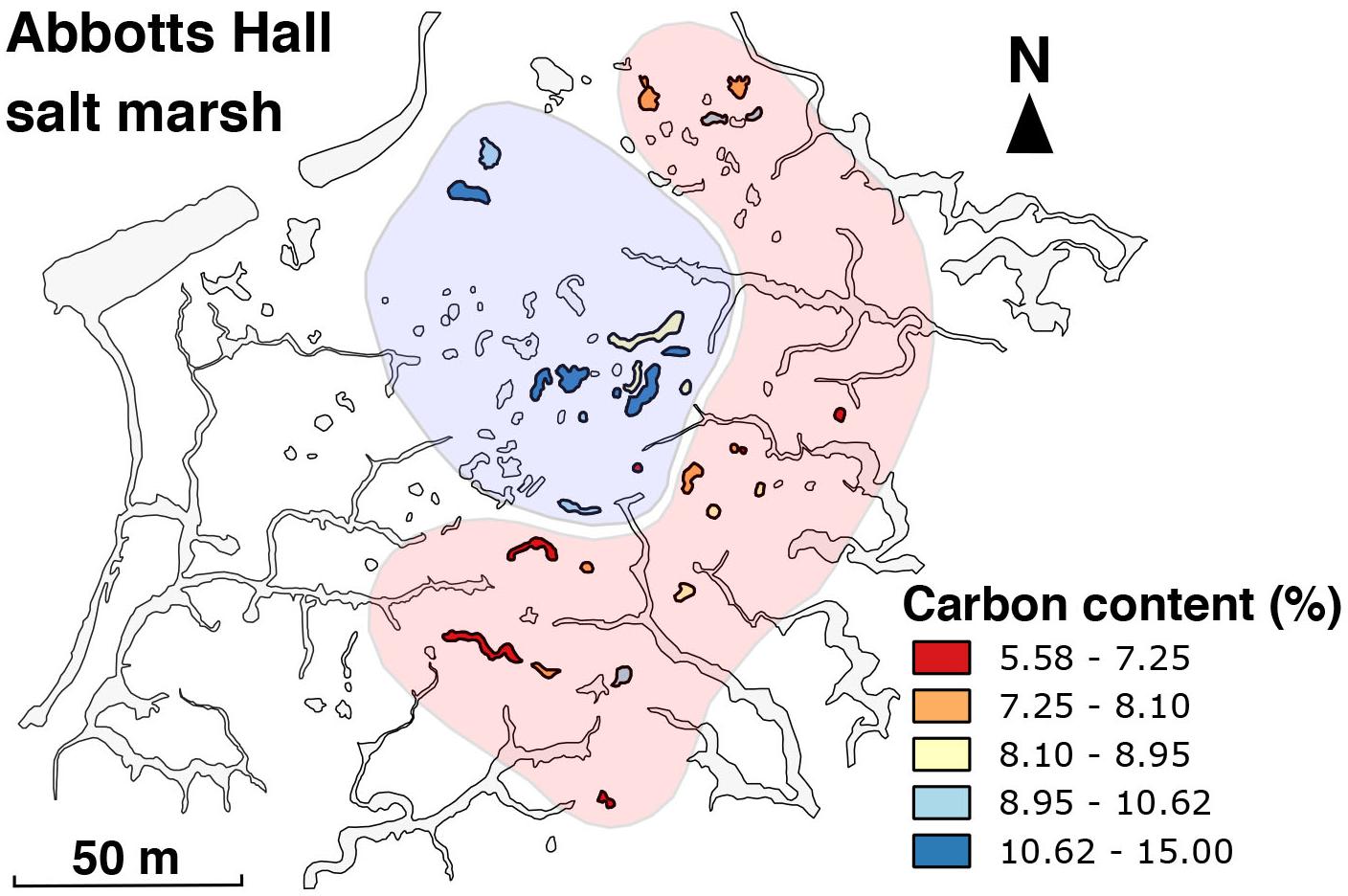
Figure 11. Distribution of organic carbon content (%) in the top 5 cm of pond sediment. Hand-drawn zones of ‘high’ and ‘low’ organic carbon content represent the overall relationship.

We hypothesize that if a pond is proximal to the creeks, it is susceptible to more flooding events and thus any organic carbon, present as dissolved organic carbon, in situ vegetation or marine algae, would be periodically flushed more regularly than ponds located centrally (Spivak et al., 2017). Additionally, the drag imparted by the rough, vegetated surfaces mean that particulate organic carbon is more likely to be deposited in the center of the platform, as the water loses energy during the ebb flow back to the creeks (Figure 12B). This mechanism may help explain why sulfide-rich ponds are located further from creeks (Figures 7, 9). On larger scales, more inland salt marsh areas would also be less affected by these flooding events due to the loss of energy of water as it travels up the platform (Figure 12B). This correlates with what we show in Figure 8, where ponds with sulfide-rich sediment are located further inland. The presence of algal debris on the surface in drone imagery (Figure 8A) reinforces this.

FIGURE 12

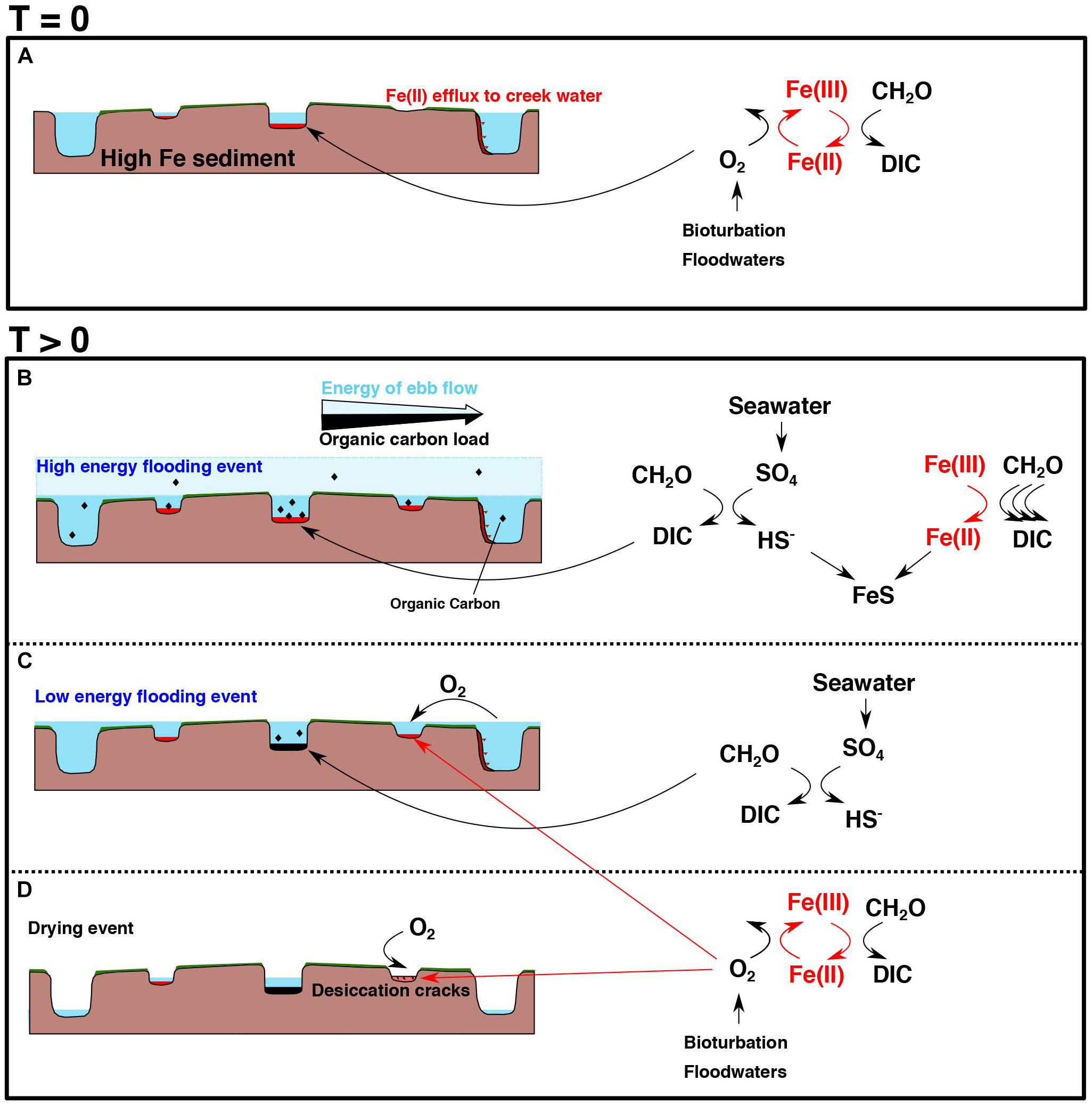
Figure 12. Schematic of potential mechanisms driving pond chemistry heterogeneity over a salt marsh platform. Vertical scale is exaggerated (likely elevation differences are within a meter). (A) Represents an earlier stage of development [T (time) = 0] in a salt marsh platform whereas (B–D) represent changes over time [T (time) > 0] (e.g., the effects of deeper, older ponds and the potential transitioning of pond sediment geochemistry). (A) Due to the high iron content of the sediment, all ponds should, in theory, have an iron-rich pond sediment geochemistry. The reaction shows bacterial iron reduction (BIR) reducing organic matter, with oxygen supplied from bioturbative-mixing and oxic flood waters, which acts to regenerate the ferrous iron. Fe(II) efflux to creek demonstrates the unknown diffusive flux at the creek wall boundary (Figure 5). (B) Periods of extremely high flooding (storm events or very high tides) from tidal creeks. All ponds are flushed with seawater and organic carbon will be deposited. As the energy of the ebb flow decreases during retreat (due to friction with the vegetated surface), the suspended organic carbon load will decrease as the flow returns to the creeks. If the central pond has sufficient organic matter to exhaust the ferric iron pool, microbial sulfate reduction can occur (see reaction alongside diagram), using seawater sulfate as the electron acceptor. This will slowly act to titrate ferrous iron as iron monosulfides, possibly acting as a switch to sulfide-rich conditions (C). (C) Low energy flooding events which may only flood ponds closer to the creeks introduces oxic water. The interior pond is assumed to have negligible available ferric iron supply so sulfide-rich pond sediment conditions are achieved. (D) Periods of excessive dry weather on the salt marsh platform (as observed in July 2018). Differential water head is attained due to the low hydraulic conductivity of the clay-rich sediment. More central ponds, having a deeper water column initially, are less susceptible to full evaporation. When the water column is fully evaporated, deep (<15 cm) desiccation cracks can occur, allowing atmospheric oxygen into the sediment. Further oxygen may be added upon submergence of the pond sediment with oxic seawater and potential bioturbating organisms.

This effect of carbon flushing will likely be convolved with the probability that more frequent flooding events add more oxygenated seawater to ponds proximal to creeks (i.e., oxygen-rich water gets added to water which has been stripped of oxygen by aerobic respiration). This would enhance aerobic respiration of organic carbon, lowering the amount of organic carbon available to sustain subsurface microbial activity (Figure 12C). More central ponds, however, are more hydrologically isolated and are less regularly flushed (Figure 12C). This allows for the in situ growth of vegetation, causing a greater organic carbon supply to the sediment (while the oxygen produced through this in situ growth would escape to the atmosphere), favoring sulfide-rich conditions. We suggest that the quantity and type of organic carbon being metabolized in different ponds and temporal studies on carbon input onto the salt marsh platform surface need to be established before we can properly understand this delivery process.

Subsurface and Surface Hydrological Flow Controls

The final hypothesis to explain the spatial distribution in the pond geochemistry is that subsurface flow, or surface flow, may play a role in distributing reactants, such as ferrous iron, to different parts of the salt marsh (see red arrows on Figure 12). This mechanism is discussed further in Antler et al. (unpublished), whereby a transient flux of ferrous iron might allow for titration of free sulfide and thus allow bioturbation to occur within pond sediments.

The large variation in ferrous iron concentrations among different iron-rich pond sediments, vegetated sediment (Figure 4) and the core taken through the creek wall (Figure 5) indicates there is heterogeneous concentration of ferrous iron over the salt marsh platform. The 3 mM decrease in ferrous iron over the 5 cm boundary layer in the creek core also suggests there is an efflux of iron out of the sediment, into the creek water. Burrowing of crabs and other organisms appears to intensify this effect. The chloride and [SO₄]/[Cl] data suggests this is hydrological mixing and not simply a zone of iron reduction. This efflux can be seen in creek water which contains up to 21 μM ferrous iron (Supplementary Table S2). From this observation, we believe that there is subsurface movement of ferrous iron over the platform, though we cannot offer insight into the direction of these flows. Hydrological flow paths in salt marshes are complex to predict; a catchment area is typically dictated over long timescales by hydrological equilibrium attained by the flood and ebb tides (Allen, 2000). This complexity could be compounded if the ponds interact with these flow paths. Additionally, surface flow likely plays some role in distributing ferrous iron leached from the sediment and deposited closer to the creeks with ebb tides. Evidence of an iron-oxide rich layer on the surface would suggest that at least some portion of this is captured upon diffusion out, though we cannot quantify this effect. Further work would be needed to test the potential of these fluxes to ‘switch’ pond sediment.

A Potential Mechanism

The mechanism which actually causes pond sediment to become sulfide-rich or iron-rich is complex. It is likely some combination of the three effects described above which, together, create conditions favorable for a certain dominant redox condition (Figure 12). Water column depth could play a role, particularly where pond sediments can become sub-aerially exposed, or where the water is so deep that atmospheric oxygen delivery to the sediment surface is greatly curtailed (Figure 12D). The correlation between water depth and classification of the pond could simply be a result of both factors being controlled by creek dynamics independently. If sea level rise causes salt marsh accretion through vegetation-induced sediment capture, then we would expect ponds being impacted by fewer flood tides—the ponds distally located from creeks—to have a lower sedimentation rate to keep pace. As such, depth distribution over the salt marsh favors deeper ponds in the center of the salt marsh platform as the system ages (Figures 12A–D). Since our data suggests a higher organic carbon content in sediments located far from creeks, there is also likely some feedback associated with organic matter degradation and a porosity increase (Spivak et al., 2017). The relative abundance of the surface fluxes of oxygen and carbon compared to the subsurface fluxes of Fe(II) and other redox available elements is important to understand whether geochemical changes are mainly imparted from the surface water or from the platform. It appears more likely based on the data presented here that the surface coupling of organic carbon and other electron acceptors acts to alter an originally iron-rich pond sediment. This is exemplified by the in situ sampler recording a change from iron-rich conditions to sulfide-rich conditions as opposed to the reverse. If this were the only mechanism, we would expect clearer boundaries of iron- and sulfide-rich pond sediment zonation. In view of this, it is likely that other processes are capable of influencing the geochemical characteristics. We suggest spatially heterogeneous transient groundwater and surface water introduction of chemical species and the evaporation of surface water introducing desiccation cracks as such processes for further exploration.

The fact that we see a zonal distribution of pond sediment chemistry implies that the change in pond chemistry is faster than rates of creek migration at present. Whilst it is thought that creek migration is actually quite slow (due to the inability of the flow to carry eroded sediment away) (Allen, 2000), if drainage ditches are emplaced, as in the northern part of Abbotts Hall, the sediment chemistry is likely to be more susceptible to change.

Conclusion

Sulfide-rich and iron-rich sediments are found throughout the East Anglian salt marshes. There is a continuum of observational evidence and porewater geochemical signatures which suggest that these classifications can encapsulate a range of geochemical behaviors. The distribution and in situ sampler data indicate that pond sediment geochemistry can be readily altered in terms of chemical classification over as short a timescale as a year. Drone based mapping of the salt marshes has shown that ponds containing sulfide-rich sediments tend to be congregated in the center of a salt marsh aggregate of ponds, further away from larger creek networks. We hypothesize that this is due to a combination of factors, including delivery of organic carbon across the salt marsh platform, variation in physical characteristics based on the position of the pond (i.e., water depth and the propensity for total evaporation), and a possible sub-surface groundwater flow distributing reactants based on position on the salt marsh. This study suggests that some combination of these effects will result in chemical heterogeneity of salt marsh pond sediment geochemistry and that no single mechanism appears dominant. The results suggest that artificial drainage ditches, common in these East Anglian salt marshes, could alter the geochemistry of these pond sediments on short timescales. This has consequences for the carbon budget, and for nutrient and trace metal capture within salt marsh ecosystems.

Data Availability

All datasets generated for this study are included in the manuscript and/or the Supplementary Files.

Author Contributions

AH wrote the manuscript. All authors contributed feedback on said manuscript. GA had the initial idea behind the study. GA and CYL collected cores for Figure 3 and provided a number of cores for Figure 4. HB, XS, and JM collected cores for Figure 4 and contributed pioneering fieldwork toward the study. MG, AH, HB, AP, and GA undertook the drone survey and subsequent characterization. JW and JC provided data for in situ sampling and AH finished the final 2 months of data analysis. AB and AH worked in the field collecting cores and undertaking subsequent analysis. KR offered insight into the Essex salt marsh system where he had worked previously. AVT is the supervisor behind all of the work involved in the salt marshes and was the first to suggest work there.

Funding

This work was funded partially by an ERC starting investigator grant (CARBONSINK – 307582) to AVT as well as NERC RG94667 to AVT. Funding for AH was provided by a NERC DTP grant (LBAG/199.02.RG91292).

Conflict of Interest Statement

The authors declare that the research was conducted in the absence of any commercial or financial relationships that could be construed as a potential conflict of interest.

Acknowledgments

The data table for this study is supplied in the Supplementary Material. This work has evolved over the course of many years and has involved the contribution of many students and scientists who have worked in the Turchyn lab and have contributed to data collection. We acknowledge in particular the help of Jiarui Lui, Katherine Halloran, and Paul Hutchings for help with fieldwork, B. Lawrence and F. Llewellyn-Beard who helped with the initial design of the in situ sampler and James Rolfe who performed carbon analysis. We acknowledge Essex Wildlife Trust for their permission for us to sample in Abbotts Hall Farm.

Supplementary Material

The Supplementary Material for this article can be found online at: https://www.frontiersin.org/articles/10.3389/feart.2019.00041/full#supplementary-material

References

Allen, J. (2000). Morphodynamics of Holocene salt marshes: a review sketch from the Atlantic and Southern North Sea coasts of Europe. Quat. Sci. Rev. 19, 1155–1231. doi: 10.1016/S0277-3791(99)00034-7

CrossRef Full Text | Google Scholar

Barbier, E. B., Hacker, S. D., Kennedy, C., Koch, E. W., Stier, A. C., and Silliman, B. R. (2011). The value of estuarine and coastal ecosystem services. Ecol. Monogr. 81, 169–193. doi: 10.1890/10-1510.1

CrossRef Full Text | Google Scholar

Bethke, C. M., Sanford, R. A., Kirk, M. F., Jin, Q., and Flynn, T. M. (2011). The thermodynamic ladder in geomicrobiology. Am. J. Sci. 311, 183–210. doi: 10.2475/03.2011.01

CrossRef Full Text | Google Scholar

Blonder, B., Boyko, V., Turchyn, A. V., Antler, G., Sinichkin, U., Knossow, N., et al. (2017). Impact of aeolian dry deposition of reactive iron minerals on sulfur cycling in sediments of the Gulf of Aqaba. Front. Microbiol. 8:1131. doi: 10.3389/fmicb.2017.01131

PubMed Abstract | CrossRef Full Text | Google Scholar

Cline, J. D. (1969). Spectrophotometric determination of hydrogen sulfide in natural waters. Limnol. Oceanogr. 14, 454–458. doi: 10.4319/lo.1969.14.3.0454

CrossRef Full Text | Google Scholar

Deegan, L. A., Johnson, D. S., Warren, R. S., Peterson, B. J., Fleeger, J. W., Fagherazzi, S., et al. (2012). Coastal eutrophication as a driver of salt marsh loss. Nature 490, 388–392. doi: 10.1038/nature11533

PubMed Abstract | CrossRef Full Text | Google Scholar

Drobner, E.H., Wächtershäuser, G., Rose, D., and Stetter, K. O. (1990). Pyrite formation linked with hydrogen evolution under anaerobic conditions. Nature 346, 742–744. doi: 10.1038/346742a0

CrossRef Full Text | Google Scholar

Froelich, P. N., Klinkhammer, G. P., Bender, M. L., Luedtke, N. A., Heath, G. R., Cullen, D., et al. (1979). Early oxidation of organic matter in pelagic sediments of the eastern equatorial Atlantic: suhoxic diagenesis. Geochim. Cosmochim. Acta 43, 1075–1090. doi: 10.1016/0016-7037(79)90095-4

CrossRef Full Text | Google Scholar

Hamblin, R. J. O., Moorlock, B. S. P., Booth, S. J., Jeffery, D. H., and Morigi, A. N. (1997). The Red Crag and Norwich Crag formations in eastern Suffolk. Proceedings of the Geologists’. Association 108, 11–23. doi: 10.1016/S0016-7878(97)80002-8

CrossRef Full Text | Google Scholar

Hansel, C. M., Lentini, C. J., Tang, Y., Johnston, D. T., Wankel, S. D., and Jardine, P. M. (2015). Dominance of sulfur-fueled iron oxide reduction in low-sulfate freshwater sediments. ISME J. 9, 2400–2412. doi: 10.1038/ismej.2015.50

PubMed Abstract | CrossRef Full Text | Google Scholar

Holmkvist, L., Ferdelman, T. G., and Jørgensen, B. B. (2011). A cryptic sulfur cycle driven by iron in the methane zone of marine sediment (Aarhus Bay, Denmark). Geochim. Cosmochim. Acta 75, 3581–3599. doi: 10.1016/j.gca.2011.03.033

CrossRef Full Text | Google Scholar

Johnston, D. T., Farquhar, J., and Canfield, D. E. (2007). Sulfur isotope insights into microbial sulfate reduction: when microbes meet models. Geochim. Cosmochim. Acta 71, 3929–3947. doi: 10.1016/j.gca.2007.05.008

CrossRef Full Text | Google Scholar

Kennish, M. J. (2016). “Anthropogenic impacts,” in Encyclopedia of Estuaries, ed. M. J. Kennish (Dordrecht: Springer), 29–35. doi: 10.1007/978-94-017-8801-4_246

CrossRef Full Text | Google Scholar

Kirwan, M. L., and Megonigal, J. P. (2013). Tidal wetland stability in the face of human impacts and sea-level rise. Nature 504, 53–60. doi: 10.1038/nature12856

PubMed Abstract | CrossRef Full Text | Google Scholar

Koretsky, C. M., Moore, C. M., Meile, C., Dichristina, T. J., and Cappellen, V. (2006). Seasonal oscillation of microbial iron and sulfate reduction in saltmarsh sediments (Sapelo Island, GA, USA). Biogeochemistry 64, 179–203. doi: 10.1023/A:1024940132078

CrossRef Full Text | Google Scholar

Lawrence, D. S. L., Allen, J. R. L., and Havelock, G. M. (2004). Salt marsh morphodynamics: an investigation of tidal flows and marsh channel equilibrium. J. Coast. Res. 201, 301–316. doi: 10.2112/1551-5036 (2004)20[301:SMMAIO]2.0.CO;2

CrossRef Full Text | Google Scholar

Lovley, D. R., and Chapelle, F. H. (1995). Deep subsurface microbial processes. Rev. Geophys. 33, 365–381. doi: 10.1029/95RG01305

CrossRef Full Text | Google Scholar

McCave, I. N. (1987). Fine sediment sources and sinks around the East Anglian Coast (UK). J. Geol. Soc. Lond. 144, 149–152. doi: 10.1144/gsjgs.144.1.0149

CrossRef Full Text | Google Scholar

Mcleod, E., Chmura, G. L., Bouillon, S., Salm, R., Björk, M., Duarte, C. M., et al. (2011). A blueprint for blue carbon: toward an improved understanding of the role of vegetated coastal habitats in sequestering CO 2. Front. Ecol. Environ. 9, 552–560. doi: 10.1890/110004

CrossRef Full Text | Google Scholar

Mills, J. V., Antler, G., and Turchyn, A. V. (2016). Geochemical evidence for cryptic sulfur cycling in salt marsh sediments. Earth Planet. Sci. Lett. 453, 23–32. doi: 10.1016/j.epsl.2016.08.001

CrossRef Full Text | Google Scholar

Mortimer, R. J. G., Galsworthy, A. M. J., Bottrell, S. H., Wilmot, L. E., and Newton, R. J. (2011). Experimental evidence for rapid biotic and abiotic reduction in salt marsh sediments: a possible mechanism for formation of modern sedimentary siderite concretions: iron reduction in salt marsh sediments. Sedimentology 58, 1514–1529. doi: 10.1111/j.1365-3091.2011.01224.x

CrossRef Full Text | Google Scholar

Nealson, K. H. (1997). Sediment bacteria: who’s there, what are they doing, and what’s new? Annu. Rev. Earth Planet. Sci. 25, 403–434. doi: 10.1146/annurev.earth.25.1.403

CrossRef Full Text | Google Scholar

Pethick, J. S. (1974). The distribution of salt pans on tidal salt marshes. J. Biogeogr. 1, 57–62. doi: 10.2307/3038068

PubMed Abstract | CrossRef Full Text | Google Scholar

Pethick, J. S. (1980). Salt-marsh initiation during the holocene transgression: the example of the north norfolk marshes, England. J. Biogeogr. 7, 1–9. doi: 10.2307/2844543

CrossRef Full Text | Google Scholar

Postma, D., and Jakobsen, R. (1996). Redox zonation: equilibrium constraints on the Fe(III)/SO4-reduction interface. Geochim. Cosmochim. Acta 60, 3169–3175. doi: 10.1016/0016-7037(96)00156-1

CrossRef Full Text | Google Scholar

Pye, K., Dickson, J. A. D., Schiavon, N., Coleman, M. L., and Cox, M. (1990). Formation of siderite-Mg-calcite-iron sulphide concretions in intertidal marsh and sandflat sediments, north Norfolk, England. Sedimentology 37, 325–343. doi: 10.1111/j.1365-3091.1990.tb00962.x

CrossRef Full Text | Google Scholar

Redfield, A. C. (1972). Development of a New England Salt Marsh. Ecol. Monogr. 42, 201–237. doi: 10.2307/1942263

CrossRef Full Text | Google Scholar

Santos, I. R., Burnett, W. C., Dittmar, T., Suryaputra, I. G. N. A., and Chanton, J. (2009). Tidal pumping drives nutrient and dissolved organic matter dynamics in a Gulf of Mexico subterranean estuary. Geochim. Cosmochim. Acta 73, 1325–1339. doi: 10.1016/j.gca.2008.11.029

CrossRef Full Text | Google Scholar

Seeberg-Elverfeldt, J., Schlüter, M., Feseker, T., and Kölling, M. (2005). Rhizon sampling of porewaters near the sediment-water interface of aquatic systems: Rhizon porewater sampling. Limnol. Oceanogr. 3, 361–371. doi: 10.4319/lom.2005.3.361

CrossRef Full Text | Google Scholar

Soetaert, K., Hofmann, A. F., Middelburg, J. J., Meysman, F. J. R., and Greenwood, J. (2007). The effect of biogeochemical processes on pH. Mar. Chem. 105, 30–51. doi: 10.1016/j.marchem.2006.12.012

CrossRef Full Text | Google Scholar

Spivak, A. C., Gosselin, K., Howard, E., Mariotti, G., Forbrich, I., Stanley, R., et al. (2017). Shallow ponds are heterogeneous habitats within a temperate salt marsh ecosystem: shallow ponds are heterogeneous habitats. J. Geophys. Res. 122, 1371–1384. doi: 10.1002/2017JG003780

CrossRef Full Text | Google Scholar

Stookey, L. L. (1970). Ferrozine—a new spectrophotometric reagent for iron. Anal. Chem. 42, 779–781. doi: 10.1021/ac60289a016

CrossRef Full Text | Google Scholar

Valiela, I., Teal, J. M., Volkmann, S., Shafer, D., and Carpenter, E. J. (1978). Nutrient and particulate fluxes in a salt marsh ecosystem: tidal exchanges and inputs by precipitation and groundwater 1: salt marsh nutrient exchange. Limnol. Oceanogr. 23, 798–812. doi: 10.4319/lo.1978.23.4.0798

CrossRef Full Text | Google Scholar

Van Huissteden, J., and van de Plassche, O. (1998). Sulfate reduction as a geomorphological agent in tidal marshes (’Great Marshes’ at Barnstaple, Cape Cod, USA). Earth Process. Landforms 23, 233–236.

Google Scholar

Wilson, C. A., Hughes, Z. J., FitzGerald, D. M., Hopkinson, C. S., Valentine, V., and Kolker, A. S. (2014). Saltmarsh pool and tidal creek morphodynamics: dynamic equilibrium of northern latitude saltmarshes? Geomorphology 213, 99–115. doi: 10.1016/j.geomorph.2014.01.002

CrossRef Full Text | Google Scholar