Actual Evapotranspiration in the High Andean Grasslands: A Comparison of Measurement and Estimation Methods

Introduction

Actual evapotranspiration (ETa) is a major component of the hydrological cycle and one of the most important physical processes in natural ecosystems. It explains the exchange of water and energy between the soil, land surface and the atmosphere. An improved characterization of ETa is especially important for: (1) the modeling and management of water resources and related ecosystem services, which include provisioning, supporting, and regulating services and (2) addressing global climate change. Climate change affects ETa rates, therefore soil moisture, vegetation productivity, the carbon cycle and water budgets might also be affected (Gu et al., 2008). Natural grasslands cover around 26% of the Earth's ice-free land surface (Foley et al., 2011). They represent a widespread ecosystem that requires special attention, as processes such as interception or transpiration have traditionally been assumed to be low or even negligible while they could in fact constitute an important loss of water to the atmosphere (Ochoa-Sánchez et al., 2018).

The most important ecosystem in the Andean region for water resources supply is the páramo and it is primarily covered by tussock grasslands (locally referred to as pajonal) (Hofstede et al., 2014). The Andean páramo extends from the North of Colombia (11°N) to the North of Peru (8°39'S), occupying around 36,000 km². The páramo geomorphology includes wide valleys covered by wetlands that act as natural reservoirs. The flora of the páramo has attracted the attention of scientists owing to the high number of endemic species. The fauna is also important for its emblematic species (e.g., condor, spectacled bear, mountain tapir, and puma). In addition, the sociological importance of the páramo lies in the millenary interaction between this ecosystem and its inhabitants. This lengthy occupation and the constant use of the páramo by nearby communities qualify it as a socio-ecosystem (Hofstede et al., 2014). The ethnic diversity of the páramo highlands promotes a lively culture that is still in development. The páramo itself is especially important as it serves as a sponge that captures precipitation and releases water gradually to the surrounding areas (Llambí et al., 2012). This characteristic is vital during dry periods or extreme summers, when water that was retained during the wet periods in the highlands is gradually delivered to lowlands through runoff. The páramo is the primary water source for communities located nearby this ecosystem, which include major cities in Colombia, Ecuador, and Peru. This environment provides water that is intensively used for agriculture, rural, and urban drinking water systems, hydro-power production, and for sustaining aquatic ecosystems. Consequently, the accurate closure of the water balance is essential. While precipitation and discharge have been increasingly monitored in the páramo (Ochoa-Tocachi et al., 2018), ETa requires further assessment.

Few studies have measured evapotranspiration in grasslands at high altitudes (Gu et al., 2008; van den Bergh et al., 2013; Knowles et al., 2015; Coners et al., 2016). In the páramo, ETa has been recently measured using the eddy-covariance (EC) method (Carrillo-Rojas et al., 2019). Although the EC method has proven to be a reliable technique, it is costly and still rarely available around the world. To our knowledge, twelve eddy-covariance towers are located in South America, among which only one is located in the páramo (Fisher et al., 2009; Carrillo-Rojas et al., 2019). This highlights the importance of finding alternative methods to quantify ETa. Weighing lysimeters have always been considered as a viable tool for measuring ETa, and as a possible alternative to the EC measurements (Coners et al., 2016). However, most of the studies focus on the use of weighing lysimeters (e.g., Rana and Katerji, 2000 and Coners et al., 2016) whose construction and operation is still costly. For that matter, some authors have constructed volumetric lysimeters as a lower-cost alternative (e.g., Khan et al., 1993 and Poss et al., 2004).

The estimation of ETa can represent an important alternative for agricultural or hydrological studies, for example when no measurement techniques are available due to their high cost, complex installation, and/or intensive maintenance. ETa has therefore been estimated through several different methods, such as using the water balance, the energy balance, the Penman-Monteith equation and hydrological models. Globally, the water balance has been used as a reference method to estimate ETa. However, the closure of the water balance involves the measurement of not only precipitation and discharge, but in some cases the measurement of other variables that are not easy to quantify, such as the change in soil moisture and groundwater recharge. The energy balance has been used to estimate ETa in the páramo, although those estimations were validated using estimations from the water balance (Carrillo-Rojas et al., 2016). The potential evapotranspiration (ETo) was estimated in the páramo through the use of the Penman-Monteith equation (Córdova et al., 2013, 2015), which is a simple method to estimate ETa that only uses a meteorological station. However, these estimations could not be validated with ETa measurements. Finally, hydrological models are a valuable estimation tool, as they are usually feasible to implement. The Probability Distribution Model (PDM) and the Hydrologiska Byråns Vattenbalansavdelning model (HBV-light) were calibrated for the páramo and have proven to be valid for runoff estimation (Iniguez et al., 2016; Sucozhañay and Célleri, 2018). Although several efforts have led to ETa estimations, they have never been compared with actual measurements.

Currently, little is known regarding which methods are suitable for accurately measuring or estimating ETa at high altitudes and, in a wider sense, studies have not compared ETa by simultaneously implementing several methods at the same site. This study therefore compares the EC measurements with low-cost volumetric lysimeters and hydrological, micrometeorological, and analytical methods that estimate ETa (i.e., water and energy balance methods, the calibrated Penman-Monteith equation and two hydrological models: PDM and HBV-light). Furthermore, this study aims to provide insights into the performance of the methods and information on the suitability of each method for similar grassland ecosystems around the globe.

Materials and Methods

Study Site

The study site is located within the Zhurucay Ecohydrological Observatory (~32 km from the city of Cuenca, Ecuador). Zhurucay is situated in a wet páramo ecosystem on the Pacific side of the Andean cordillera (Figure 1) and is an open-field laboratory where hydrological, micrometeorological, and ecological research is conducted. It has a drainage area of 7.36 km² and the elevation ranges from 3,500 to 3,900 m (a.s.l.). Annual precipitation is around 1,200 ± 100 mm and the precipitation regime is divided into wet (January to May and October) and dry months (June to December). The climate is influenced by the west Pacific regime and the air masses from the Amazon (Córdova et al., 2013). The mean annual temperature is 6°C, the mean relative humidity is 91%, the mean solar radiation is 14 MJ/m²/day, and the mean wind speed is 3.6 m/s (Córdova et al., 2015). The vegetation consists mainly (>80%) of tussock grasses (Calamagrostis Intermedia (J. Presl) Steud. sp., commonly known as “pajonal”), which are perennial plants that grow in bunches leaving no bare soil at the study site. Soils correspond mainly to Andosols with a minority of Histosols (24%) (FAO/ISRIC/ISSS, 1998).

FIGURE 1

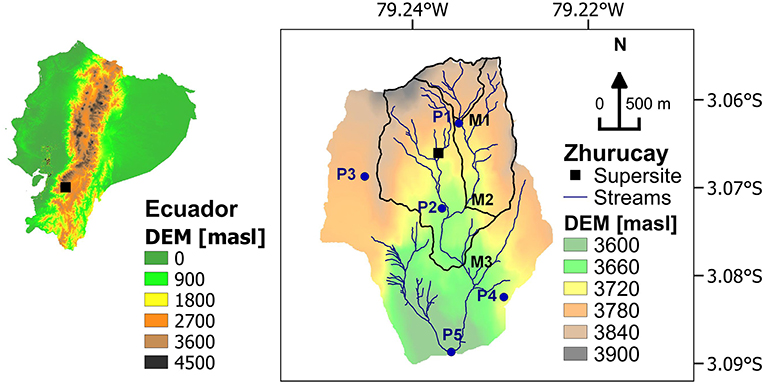
Figure 1. Zhurucay Ecohydrological Observatory located in Southern Ecuador. Three main microcatchments within the Zhurucay Observatory are numbered from M1 to M3 and five rain gauges are numbered from P1 to P5.

A monitoring supersite exists at Zhurucay (Figure 1), equipped with micrometeorological sensors such as an eddy-covariance tower, a meteorological station, energy fluxes sensors, precipitation sensors (rain gauges and a laser disdrometer), as well as a hillslope equipped with a set of 38 water content reflectometers (WCRs).

Methods for Measuring and Estimating Actual Evapotranspiration

Rose and Sharma (1984) suggested that methods should be grouped as those that measure ETa and those that estimate ETa. In addition, methods may be classified as experimental and physically-based. Each method has been developed based on certain assumptions and to fulfill a different objective, therefore each depends on concepts from hydrology or micrometeorology. Among the methods used in this study, eddy-covariance and lysimeters measure ETa, while the water balance method, energy balance method, the hydrological models and the calibrated evapotranspiration equation estimate ETa. Volumetric lysimeters and the water balance method depend on hydrological concepts, while the energy balance and eddy-covariance methods are micrometeorological approaches. The calibrated evapotranspiration equation and the estimation through hydrological models can be grouped as analytical approaches.

All methods have a different time and spatial resolution, as summarized in Table 1. In this study all methods were compared on a daily timescale over a period of 1 year (05/05/2017–30/04/2018), which included comprehensive field campaigns, especially for the implementation of the eddy-covariance tower and the lysimeters.

TABLE 1

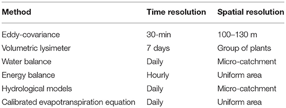
Table 1. Spatial and temporal resolution of the actual evapotranspiration measurement and estimation methods used in this study.

Eddy-Covariance Method (ETa_EC)

Water vapor and energy fluxes were measured by an EC tower from May 2017 to April 2018. The EC site is a FLUXNET observatory (ID: EC-Apr). A photograph of the EC tower is shown in Supplementary Figure 1A. A LI-7200 enclosed-path infrared gas analyzer (LI-COR, Lincoln, NE, USA) detected ETa fluxes at a sampling rate of 20 Hz. The analyzer used an insulated heated tube to avoid water condensation during the sampling intake. Wind components and the sensible heat flux were measured using a three-dimensional sonic anemometer (Gill New WindMaster 3D, Gill Instruments, Hampshire, UK). Additional micrometeorological measurements were taken with slow sensors (with a 1 min sampling frequency) collecting net radiation data (Kipp & Zonen CNR4, Delft, Netherlands), air temperature and relative humidity levels (Vaisala HMP155, Helsinki, Finland), and soil heat fluxes (3 × Hukseflux HFP01, Delft, Netherlands; buried at 8 cm in the soil). The array of instruments was set up at a 3.6 m elevation, surveying the grassland fetch up to ~100–130 meters in the prevailing upwind direction of the flux source (northeast). The ET flux contributions developed from a homogeneous cover of tussock grassland with low orographic affectation (<10°). Detailed characteristics of this pioneering high Andean EC experiment have been described in Carrillo-Rojas et al. (2019).

High-frequency sampling data (ETa and sensible heat) were 30-min block averaged using the EddyPro software (version 6.2.0, LI-COR, Lincoln, NE, USA). The raw data processing contemplated diagnostic flags, plausibility limits, and spike removal. In addition, data quality assurance and quality control were performed, along with corrections for density fluctuations, time lags, wind planar fit, and high- and low-frequency spectral losses, following the recommendations of Mauder et al. (2013). Footprint assessment, based on the methodology of Kljun et al. (2015), excluded <2% of flux data related to unimportant sources in the area, and the EC energy balance closure amounted to 99% in the studied period. This outstanding closure of the energy balance is attributed to the smooth and homogeneous canopy of the native vegetation, the constant moist conditions and the particular location of our site (tropical latitude with low seasonality). Other tropical sites with high moisture environments have shown similar energy balance closures (Cabral et al., 2010, 2015). Advection-affected fluxes were removed through the detection of data with low friction velocity (u*). This was performed using the Moving Point Test for the u* threshold detection (Papale et al., 2006). Missing ET fluxes (scarce temporal gaps of <1 day), due to the u* filtering or power or instrumental failures, and low quality data amounted to 23% of the total amount of 30-min data. This represents a good level of EC temporal coverage according to Falge et al. (2001). These data gaps were filled using the standard method used in FLUXNET, i.e., Marginal Distribution Sampling (MDS) (Reichstein et al., 2005). We selected such an approach due to its wide application at other EC sites and to maintain consistency with former and future studies. The MDS algorithm infilled the missing values with solar radiation, air temperature, and vapor pressure as input variables. The uncertainty error induced by gap filling was assessed using a bootstrapping approach (resampling with replacement). A dataset of pseudo-replicates was created. Here, the difference between the high (95% quantile) and low (5% quantile) threshold estimates of the bootstrapped uncertainty distribution corresponded to the uncertainty level. A detailed description of the EC data processing and specific corrections can be found in Carrillo-Rojas et al. (2019).

Lysimeters Installation and Methodology

Four volumetric lysimeters were installed at the top of the hillslope at the supersite, as depicted in Figure 2a. Actual evapotranspiration (ETa_Lys) was calculated by closing the water balance for each lysimeter as in Equation 1:

$\begin{array}{ll}ET{a}_{Lys}=P-D\pm \Delta S& (1)\end{array}$

where P corresponds to precipitation (in mm/7 days), D corresponds to drainage (in mm/7 days), and ΔS is the change in soil water storage (in mm/7 days). The lysimeter illustration depicted in Figure 2b indicates the design and instrumentation used for the closure of the water balance. Lysimeters contain only the organic horizon and the bedrock is located immediately below the instruments. First, precipitation was recorded with a laser disdrometer (Thies Clima Laser Precipitation Monitor 5.4110.00.000 V2.4 × STD, with 0.01 mm resolution). Changes in soil water storage were calculated from the difference between two WCRs installed inside the lysimeters (CS655 Campbell Scientific WCRs). Changes in soil water tension and soil water potential were continuously checked with tensiometers (T8-UMS) and dielectric water potential sensors (MPS-2 Decagon). Drainage was obtained by placing fiberglass wicks at the bottom of the lysimeters. The wicks acted as a hanging water column, drawing water from the undisturbed field soil without external application of suction (Boll et al., 1992). Lysimeters were sealed laterally and at the bottom, leaving only a central output in the base (2 cm in diameter) for connecting one end of the wick internally through a flexible tube pipe that ends in a rain gauge (TE525MM, Texas, with 0.1 mm resolution). Tips recorded by the rain gauge were corrected for the real collection area, which corresponded to the lysimeter circular area. The daily water balance of the lysimeters frequently gave negative values of ETa. Values were therefore aggregated and a 7-day water balance was found to be sufficient to allow precipitation/drainage balance, and thus only positive values of ETa remained. A weekly closure of the lysimeters' water balance was therefore selected for this study.

FIGURE 2

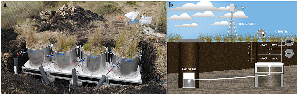
Figure 2. (a) Lysimeters installed at the study site before they were covered by soil and vegetation. Sensors shown are T8 tensiometers. (b) Illustration of the lysimeter instrumentation (WCR, water content reflectometers; DWP, dielectric water potential sensors; T8, tensiometers). Dimensions are shown in centimeters.

Water Balance Method

The water balance was closed for each of three microcatchments M1, M2, and M3 (Figure 1) as in Equation 2:

$\begin{array}{ll}ET{a}_{WB}=P-Q\pm \Delta S& (2)\end{array}$

where P is precipitation (in mm/day), Q is discharge (in mm/day), and ΔS is the change in soil water storage (in mm/day). Precipitation for each microcatchment (M1–M3) was calculated with Thiessen polygons (Jones and Hulme, 1996) from five rain gauges (4 ONSET and one Texas TE525MM). Discharge was registered by using V-notch weirs installed at the outlet of the microcatchments. The change in soil water storage was estimated via the daily difference in the storage calculated with soil moisture data from ten WCRs (CS616 Campbell Scientific WCRs) located at five depths (10, 25, 35, 60, and 70 cm) on the supersite hillslope (Figure 1). Daily storage was calculated by integrating the storage of the mineral and organic soil depths located at five hillslope topographic positions classified in Table 2. The daily storage of catchment M1 at the toe slope position, for example, corresponds to 1.87% (calculated as: area percentage of the toe slope position × [(400 × VWC) (i.e., the organic soil depth × the soil volumetric water content (VWC), which is here the average of the WCRs located at the toe slope position and at the organic soil depth) + (300 × VWC) (i.e., the mineral soil depth × soil VWC, which is here the average of the WCRs located at the toe slope position and at the mineral soil depth)]. All hillslope topographic positions were calculated in this manner and summarized, giving the daily storage of the M1 area.

TABLE 2

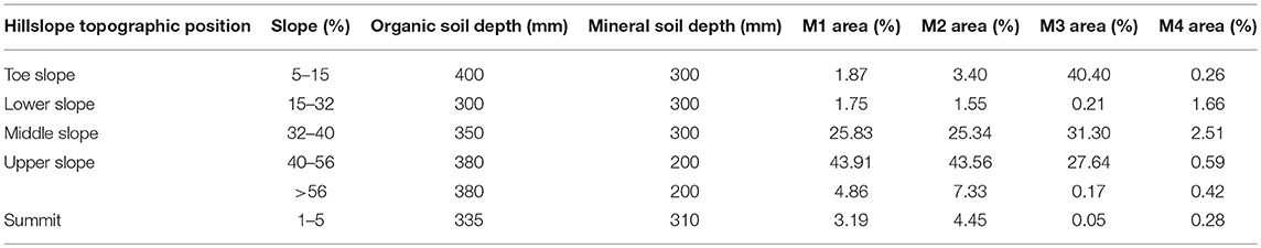
Table 2. Zhurucay microcatchments soil characteristics.

Microcatchments M1–M3 differ mainly by their size. Their vegetation cover, soil type properties and hydrological characteristics are described in Supplementary Table 1.

Energy Balance Method

Actual evapotranspiration is equivalent to the latent heat flux variable (LE, in mm/hour), which is used in the Earth's surface energy budget (Monson and Baldocchi, 2014). It is defined as the amount of energy necessary to transform liquid water into vapor, and was therefore converted to the amount of water that is evaporated or transpired from the Earth's surface. Thus, actual evapotranspiration (ETa_EB) can be calculated with the energy balance presented in Equation 3:

$\begin{array}{ll}ET{a}_{EB}=LE=Rn-G-H& (3)\end{array}$

where Rn is the net radiation (in mm/hour), G is the ground heat flux (in mm/hour) and H is the sensible heat flux (in mm/hour).

Rn was measured immediately above the vegetation height at around 0.6 m, by averaging two net radiometers (CNR4 Kipp & Zonen) located on the hillslope of the Zhurucay supersite. In order to calculate G, two pairs of soil heat flux plates (HFP01SC Campbell Scientific) were located at 8 cm depth from the soil surface (one pair below each net radiometer). G was calculated as the average of the soil heat flux plates plus the heat storage estimation of Mayocchi and Bristow (1995). Therefore, each plate was installed together with a water content reflectometer (CS616 Campbell Scientific) and soil temperature probes (TCAV). H was estimated with the flux variance method detailed in Wesson et al. (2001), in order to calculate it from available meteorological variables without including any complex or uncommon methods such as the eddy-covariance method. The flux variance method calculates H with the following input variables that were measured by the meteorological station: mean air temperature T (CS-2150 Campbell Scientific), mean wind speed u₂ (Met-One 034B Windset anemometer), and net radiation Rn (CNR4 Kipp & Zonen). Since the flux variance method uses different equations for calculating H during day-time and night-time hours, we chose an hourly timestep for the energy balance method. Photographs of the net radiometer, heat flux plates, water content reflectometer, TCAV and meteorological station are shown in Supplementary Figure 1.

Potential Evapotranspiration Equation Calibrated With Eddy-Covariance Measurements

The American Society of Civil Engineers (ASCE) through its Water Resources Institute Technical Committee (ASCE-ET) selected the alfalfa-basis model ASCE Penman-Monteith equation (ASCE-PM) for standardization of the potential evapotranspiration estimation (Walter et al., 2000). Equation 4 presents the ASCE-PM equation in its reduced form, including Cn and Cd, which represent the numerator and denominator parameters that change with vegetation reference type and calculation time-step. These parameters were calibrated in this study for the páramo vegetation at a daily timescale. The calibration procedure compared 2-year daily data (01/05/2016–30/04/2018) from the eddy-covariance measurements with the corresponding values of actual evapotranspiration estimated with the ASCE-PM calibrated equation (ETa_PMCal). The parameters Cn and Cd vary over the ranges 0–1,000 and 0.25–1, respectively. The best values of the parameters were found by randomly creating 5,000 values for each parameter inside the given ranges. The values with the lowest bias, the lowest normalized root mean square error (nRMSE) and the highest Pearson's correlation coefficient (r) were then selected. The 10-fold cross-validation method was then used to prove whether the equation could be used with a different dataset. The method was implemented by partitioning the total number of ETa values (368) into ten groups. As 368 divided by 10 does not give an integer result, nine groups had 36 values and the last group had 44 values. The function (Equation 4) was then applied ten times and one group was left out for fitting at each iteration. The fitted values were compared with the observed values using the coefficient of determination (R²).

When Equation 4 is used with Cn = 900 and Cd = 0.34, the result gives the Penman-Monteith potential evapotranspiration (ETo), which was also calculated for the period of this study in order to provide the estimates of evapotranspiration when there is no water distress:

$\begin{array}{ll}ET{a}_{PMCal}=\frac{0.408\Delta (R_n-G)+\gamma \frac{C_n}{T+273}{u}_2(e_s-e_a)}{\Delta +\gamma (1+C_d{u}_2)}& (4)\end{array}$

where Rn is the net radiation (in MJ/m²/day), G is the soil heat flux density (in MJ/m²/day) (which tends to be zero after 24 h), T is the mean air temperature at 2 m elevation (in °C), γ is the psychrometric constant (in kPa/°C), u₂ is the mean wind speed at 2 m elevation (in m/s), e_s is the saturation vapor pressure at 2 m elevation (in kPa), e_a is the mean actual vapor pressure at 2 m elevation (in kPa), and Δ is the slope of the saturation vapor pressure-temperature curve (in kPa/°C).

Hydrological Models

The hydrological models PDM and HBV-light were run for the M1 microcatchment (Figure 1). The M1 microcatchment is the most similar to the EC footprint compared to the M2 or M3 microcatchments, in terms of the altitude, soil type distribution and vegetation coverage (see Supplementary Table 1). The following input variables were measured at the Zhurucay meteorological station (see Supplementary Figure 1D): daily precipitation P (calculated with Thiessen polygons from five rain gauges: 4 ONSET and one Texas TE525MM, Figure 1), daily potential evapotranspiration ETo (see section Potential evapotranspiration equation calibrated with eddy-covariance measurements), and daily mean air temperature T (CS-2150 Campbell Scientific).

The probability distribution model (PDM) (Moore and Clarke, 1981; Moore, 1985) was calibrated at a nearby catchment (~2 km from the Zhurucay supersite) and proved to work-well for estimating slow flows and evapotranspiration (Iniguez et al., 2016). Thus, the parameters calibrated and validated by Iniguez et al. (2016) were used to estimate actual evapotranspiration during the period of this study. The PDM model was implemented within a MATLAB toolbox using the options of calculating the actual evapotranspiration ETa_PDM as a function of the potential evaporation and the soil moisture deficit [S_max-S(t)] by Wagener et al. (2001), as in Equation 5:

$\begin{array}{ll}ET{a}_{PDM}=\left\{1-\left[\frac{S_{\mathit{\text{max}}}-S(t)}{S_{\mathit{\text{max}}}}\right]\right\}\times ETo& (5)\end{array}$

The Hydrologiska Byråns Vattenbalansavdelning model, in its HBV-light version, is a semi-distributed model (Bergström, 1976), which was calibrated and validated at Zhurucay (Sucozhañay and Célleri, 2018). The HBV-light was run at the M1 microcatchment with the same parameterization. Actual evapotranspiration from the soil box equals the potential evaporation if the current soil water storage [S(t)] over the maximum soil water storage (S_max) is above the parameter threshold for reduction of evaporation (P_LP) multiplied by the S_max, while a linear reduction is used when S(t) over S_max is below this value (Equation 6):

$\begin{array}{ll}ET{a}_{HBV}=ETo\times min\left(\frac{S(t)}{S_{max}\times P_{LP}},1\right)& (6)\end{array}$

Comparison of Actual Evapotranspiration Measurements and Estimates

Eddy-covariance and lysimeters both measure actual evapotranspiration. They were therefore considered as the references to which the estimation methods should be compared. However, the volumetric lysimeters used in this study have a lower temporal resolution than the eddy-covariance method (7-days compared to 30 min), and the eddy-covariance measurements were therefore preferred for the comparison in order to analyze all the methods on a daily basis. To analyze the lysimeter performance, the EC measurements were aggregated to 7 days.

First, daily averages of ETa_EC for each month were examined together with precipitation data in order to characterize ETa seasonally. The daily comparison between methodologies was assessed by accumulating the measurements and estimates during 1 year, then plotting daily ETa boxplots of the measurements and estimates, and calculating daily statistics such as the bias percentage (pbias), the normalized root mean square error (nRMSE), Pearson's correlation coefficient (r), the volumetric efficiency (ve), and the coefficient of determination (R²). Finally, daily differences between the different methods and the EC measurements were plotted.

The bias percentage (Equation 7) measures the average tendency of the daily ETa estimations (sim) to be larger or smaller than the daily EC measurements (obs). It should be taken with caution as it compensates over-estimations with under-estimations at the end of the year. RMSE is commonly used for model performance applications to calculate positive errors. However, the RMSE is sensitive to outliers and extreme values as deviations are squared. The nRMSE (Equation 8) was therefore used instead. The Pearson's correlation coefficient (Equation 9) was calculated to measure the linear correlation between estimates and measurements, however it is sensitive to outliers. To overcome the problem with the compensation of over- and under- estimations and the sensitivity to outliers and extreme values, the ve was also selected (Equation 10). The ve has been proposed as an alternative to the Nash-Sutcliffe Efficiency and has been suggested to be complementary to other metrics, with the advantage that it eliminates the squaring of the deviations (Criss and Winston, 2008). The values of ve range from 0 to 1 and represent the fraction of water delivered at the proper time. In addition, the coefficient of determination R² (Equation 11) was chosen to estimate the proportion of the variance in the ETa measurements that can be predicted from the ETa estimates. All metrics were computed with the hydroGOF package of R, version 3.5.1:

$\begin{array}{ll}pbias=100\frac{{\displaystyle {\sum }_{i=1}^n}si{m}_i-ob{s}_i}{{\displaystyle {\sum }_{i=1}^n}ob{s}_i}& (7)\end{array}$

$\begin{array}{ll}nRMSE=100\frac{\sqrt{\frac{1}{n}{\displaystyle {\sum }_{i=1}^n}{(si{m}_i-ob{s}_i)}^2}}{ob{s}_{max}-ob{s}_{min}}& (8)\end{array}$

$\begin{array}{ll}r=\frac{cov(sim,obs)}{{\sigma }_{sim}{\sigma }_{obs}}& (9)\end{array}$

$\begin{array}{ll}ve=1-\frac{{\displaystyle {\sum }_{i=1}^n}|si{m}_i-ob{s}_i|}{{\displaystyle {\sum }_{i=1}^n}ob{s}_i}& (10)\end{array}$

$\begin{array}{ll}{R}^2=\frac{{\displaystyle {\sum }_{i=1}^n}{\left(si{m}_i-\overline{obs}\right)}^2}{{\displaystyle {\sum }_{i=1}^n}{\left(ob{s}_i-\overline{obs}\right)}^2}& (11)\end{array}$

where n is the total number of daily ETa values, sim is the corresponding daily ETa estimate from each method, obs is the ETa_EC measurement, obs_max is the maximum ETa_EC value, obs_min is the minimum ETa_EC value, cov is the covariance between daily ETa measurements and estimates, and σ is the variance.

Furthermore, in order to discuss the performance of each method, the following approaches were taken:

• Lysimeters: the cumulative ETa for each lysimeter was plotted together with the change in storage;

• Water balance: ETa_WB for each catchment (M1–M3), with and without the ΔS term, were compared with EC measurements;

• Energy balance: each term of the balance equation was compared with the terms measured by the eddy-covariance method;

• Hydrological models: the soil water storage calculated by each model was compared with WCRs observations at the Zhurucay supersite, in terms of the variations throughout the year.

Results

Measuring Daily Actual Evapotranspiration With the Eddy-Covariance Method

Eddy-covariance measurements of daily actual evapotranspiration are shown for every month from May 2017 to April 2018 in Figure 3. The daily ETa varied little throughout the year, with a minimum median of 1.3 mm/day in July and a maximum median of 2.0 mm/day in February. The minimum ETa value was 0.3 mm/day and the maximum value was 4.0 mm/day. The mean ETa for the entire year was 1.7 mm/day. ETa boxplots in Figure 3 show a higher variance for July, September, October, November, January, and February. Variables that are important for the evapotranspiration process, such as net radiation, precipitation, volumetric soil water content, potential evapotranspiration, and relative humidity, are also shown in Figure 3. The ETa distribution, median ETo, and median Rn were plotted together, showing a similar variability throughout the year. The ETa was on average 13% lower than the daily ETo.

FIGURE 3

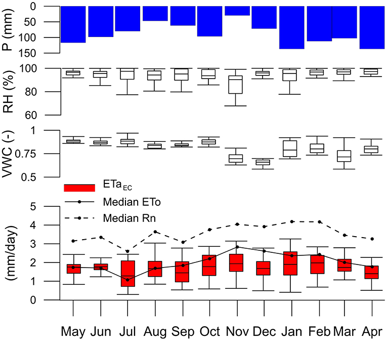
Figure 3. Daily actual evapotranspiration measured with the eddy-covariance method (ETa_EC in mm/day) shown for every month together with the median potential evapotranspiration (ETo in mm/day) estimated with the Penman-Monteith equation and median net radiation (Rn in mm/day). Additionally, monthly precipitation (P in mm/month), soil volumetric water content (VWC), and relative humidity (RH in percentage) are shown.

Comparison of Methods for Estimating and Measuring Actual Evapotranspiration

Cumulative values of daily actual evapotranspiration (for every method), daily potential evapotranspiration, and daily precipitation are shown in Figure 4. The EC measurements recorded 622 mm of actual evapotranspiration at the end of 1 year, while cumulative precipitation was 1,094 mm. In general, all methods except the calibrated evapotranspiration equation underestimated ETa throughout the year. At the end of the year, the calibrated evapotranspiration equation, water balance, and lysimeters were the most accurate in estimating annual ETa (with a 3–10% underestimation), while the other methods underestimated annual ETa by around 20%. The EC and the PMCal methods found an ETa/P-value equal to 0.57, while the other methods found an ETa/P-value equal to 0.5. This indicates that a little more than a half of the precipitation returns to the atmosphere by either evaporation or transpiration. Similarly, the EC and PMCal methods found that the ETa/Rn evaporative fraction was equal to 0.48, while the other methods underestimated this value (the lysimeters and water balance method found ETa/Rn = 0.44, while the hydrological models and the energy balance method found ETa/Rn = 0.40). This indicates that almost half of the energy available at the surface was used for evaporation and transpiration.

FIGURE 4

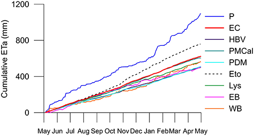
Figure 4. Cumulative daily actual evapotranspiration measured by the eddy-covariance (EC) and lysimeters (Lys) and estimated by the PDM and HBV-light hydrological models, the water balance (WB) and energy balance (EB) methods, the calibrated evapotranspiration equation (PMCal), and the potential evapotranspiration (ETo). Cumulative precipitation (P) is also shown.

Daily measurements of actual evapotranspiration by the EC method are shown in Figure 5 as a boxplot for the entire year. Boxplots of daily ETa estimates from the hydrological models (HBV-light and PDM), water and energy balance methods, and the PMCal equation are also shown. The hydrological models and the PMCal were the most similar to the EC measurements distribution. The energy balance estimates had a very similar median to the EC measurements but the variance was much higher. The water balance estimates were the least similar to the EC measurements out of all methods, with a lower median and a very different distribution. These results were corroborated with the bias percentage (pbias), the normalized root mean square error (nRMSE), the Pearson's correlation coefficient (r), the volumetric efficiency (ve), and the coefficient of determination (R²), which are shown for all methods in Table 3. The bias percentage of all the methods in comparison with the EC measurements were, from lowest to highest: −3% for the calibrated evapotranspiration equation (PMCal), −10% for the lysimeters, −10% for the water balance method, −18% for the PDM model, −19% for the energy balance, and −20% for the HBV-light model. Regarding error and correlation, the hydrological models and the PMCal presented, on a daily basis, the best performance with the lowest error (12–15%), the highest correlation (r = 0.7–0.9 and R² = 0.5–0.8), and the highest efficiency in estimating the water volume (ve = 0.8).

FIGURE 5

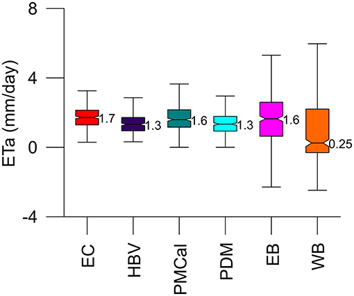
Figure 5. Daily actual evapotranspiration measured by the eddy-covariance method (EC) and estimated by the HBV-light and PDM models, the calibrated evapotranspiration equation (PMCal), the energy balance (EB) and the water balance methods (WB).

TABLE 3

Table 3. Bias percentage (pbias), normalized root mean square error (nRMSE), Pearson's correlation coefficient (r), volumetric efficiency (ve), and coefficient of determination (R²) for the actual evapotranspiration estimated with the HBV-light and PDM models, the calibrated evapotranspiration equation (PMCal), the lysimeters (Lys), the energy balance (EB), and water balance (WB) methods against the eddy-covariance measurements.

Finally, Figure 6 shows the daily differences between the methods and the EC measurements. The hydrological models and the calibrated evapotranspiration equation were biased from the EC measurements over a range −2 to 2 mm/day, the energy balance method was biased over a range −12 to 4 mm/day, the lysimeters were biased over a range −12 to 6 mm/day, and the water balance method was biased over a range −6 to 14 mm/day. Remarkably, the HBV-light outperformed the rest of the models while the water balance method was the one that presented major differences in comparison with the EC measurements. Although the water balance and lysimeters had the second lowest bias percentage throughout the year (Table 3), the differences shown in Figures 3, 6 suggest that this value is the result of the compensation of the considerable over- and under-estimation of daily differences. Thus, these methods estimate ETa better than other methods at the end of the year, but fail at estimating ETa on a daily or weekly basis.

FIGURE 6

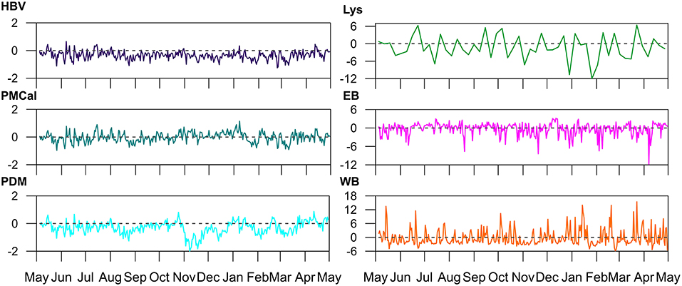
Figure 6. Daily differences in evapotranspiration between the methods and the eddy-covariance (in mm). Methods include: PDM and HBV-light hydrological models, lysimeters (Lys), energy balance (EB), water balance (WB), and the calibrated evapotranspiration equation (PMCal).

Overall, these results indicate that the hydrological models and the calibrated evapotranspiration equation are the most efficient methods for estimating daily ETa when compared with the EC measurements.

Discussion

Actual Evapotranspiration and Its Environmental Controls

Actual evapotranspiration in the páramo was 1.7 mm/day on average (ranging from 0.3 to 4.0 mm/day) according to the EC measurements. ETa has rarely been measured or estimated in the páramo or at high altitudes, such as at 3,765 m a.s.l. where the EC tower and the lysimeters are located. At a nearby location, Iniguez et al. (2016) modeled ETa with the PDM and found slightly lower daily averages of 1.47 mm/day (ranging from 0.19 to 3.33 mm/day). At 3,250 m in the Tibetan meadows, Gu et al. (2008) measured ETa with the EC method and found daily values of 4 mm (ranging from 1.9 to 6 mm) for 30 cm herbaceous vegetation with almost no bare soil (90% vegetation coverage). Coners et al. (2016) measured at the same site a daily ETa range of 1.9–2.2 mm/day with EC and lysimeters. Nevertheless, the ETa/P ratio found in this study (0.57) is similar to the studies mentioned previously (0.6–0.7) and is slightly lower than the mean terrestrial ratio (0.66) (Oki and Kanae, 2006). Also, at New Zealand sites Campbell and Murray (1990) and Holdsworth and Mark (1990) registered an ETa/P ratio between 0.2 and 0.5, where the tussock grasslands are very similar to our site despite a lower altitude of around 1,000 m (a.s.l.). In Peru, similar daily ETa values were found for puna grasslands (ranging from 1.5 to 2.3 mm/day). However, given the high precipitation at that site, the annual ETa/P ratio was 0.2 (Clark et al., 2014). Finally, Fisher et al. (2009) found ETa values of 1,096 mm/year from eddy-covariance towers located in the Amazonian rainforest in the tropics. The ETa values presented here for the páramo should be added to that synthesis study.

The ETa amount depends mainly on water and energy availability. As precipitation (P) and the soil VWC (VWC) are high at the study site (Figure 3), high rates of drizzle have been measured (Padrón et al., 2015) and high interception rates during low intensity events have been quantified (Ochoa-Sánchez et al., 2018), sufficient water is available for evaporation and transpiration almost all year long. Regarding the available energy, Figure 3 shows that the variability of ETa is the same as that of ETo and Rn. ETa was found, on average, to be 13% lower than ETo and this indicates an evaporative fraction of 0.48. Moreover, an important characteristic of our site is the high relative humidity present in the páramo that keeps the air saturated or almost saturated, thus no additional vapor is allowed in the atmosphere (Figure 3). This is corroborated by the high differences in ETa/P between wet and dry months (0.46 and 0.95 on average, respectively). During dry months (<100 mm/month), although less water is available for evapotranspiration, lower cloudy conditions allow higher radiation (Figure 3), and consequently more evaporation. The opposite occurs during wet months.

In summary, the constant rainfall balances ETa loss and drainage. A similar water balance was also found for native tussock grassland catchments in New Zealand (Bowden et al., 2001). There is practically no time in the year where the soil VWC drops below 0.7 (field capacity), except during drier months when values of 0.6 were recorded. However, these values are not below the wilting point (0.45).

Sources of Uncertainty in the ETa Estimation Methods

In general, the ETa was underestimated by all methods except the PMCal equation (Table 3, Figure 5). Volumetric lysimeters were the most accurate in closing the water balance at the vegetation scale, as they used disdrometer observations to measure P and also took into account the change in soil water storage (ΔS). However, disdrometer measurements were only available at the supersite, therefore the water balance and the hydrological models used rain gauge measurements for quantifying P. In addition, the water balance did not include the ΔS term. Here, we showed that the water balance and lysimeters are good at estimating ETa by the end of the year while hydrological models were the most correlated with EC measurements, although they underestimated ETa by the end of the year. During the time period of the comparison, the daily disdrometer measurements recorded 4% more rainfall than rain gauge measurements and they showed a difference of 10% in absolute daily values. If we assume homogeneity between the supersite and microcatchments inside Zhurucay, disdrometer measurements of P could improve the water balance estimation of annual ETa.

Due to the similarities between the ETa and ETo during the first months of this comparison period (May–August), as ETa seems to be limited by the energy availability and not by water availability, the energy balance was very close to the cumulative values of EC measurements (Figure 4). In addition, the outstanding performance of the PMCal (Table 3) is due to the calibration with the EC measurements that served as a bias correction for ETo.

Scatterplots of each ETa measurement and estimation method against one another are given in Supplementary Figure 2. These plots confirm the high performance of HBV-light, PMCal, and PDM estimates, which are positively and highly correlated with the EC measurements (r = 0.88, 0.66, and 0.72, respectively). These methods are also correlated amongst themselves. In addition, the net radiation (Rn) was the meteorological variable that showed the highest correlation with the EC measurements, compared to other variables such as the relative humidity, wind speed, soil moisture, air temperature, and precipitation. This agrees with the studies of Córdova et al. (2015) and Fisher et al. (2009). Fisher et al. (2009) found that Rn was the strongest determinant of evapotranspiration in the tropics. Rn daily values are plotted against the ETa measurements and estimations in Supplementary Figure 2, showing a high correlation with the EC measurements (r = 0.88) and the HBV-light, PMCal and PDM estimates (r = 0.88, 0.74, and 0.71, respectively).

In the following sections, the sources of uncertainties from each method are discussed.

The Eddy-Covariance Technique

The eddy-covariance method applied to non-ideal surfaces, such as steep terrain, and harsh environments can present uncertainties (Baldocchi, 2003). The main sources of biases are related to night-time advection (mostly related to carbon dioxide and methane fluxes, rather than ETa) (Novick et al., 2014) and to the energy exchange that is affected by the underlying sloped surface (Serrano-Ortiz et al., 2016). Such uncertainties cannot be accounted for in the present study, due to the need for additional sensors. However, the uncertainties induced by the data gap-filling process have been calculated via a bootstrapping technique, and amounted to 0.002 ± 0.008 mm/h (1.3%) of the hourly ETa mean for the gap-filled data values exclusively (~20% of the total dataset).

Lysimeters

Four volumetric lysimeters measured ETa over a period of 1 year by closing the water balance every seven days. The variables involved in the water balance are precipitation, drainage, and storage. Precipitation measured with the disdrometer (with a resolution of 0.01 mm) includes observations of light-rain and drizzle, commonly present in the páramo. However, the cumulative drainage differed greatly between lysimeters (up to 165 mm) by the end of the year. Consequently, the ETa measured with each lysimeter differed in a similar manner. This difference represented 38% of the total cumulative ETa. The uncertainty between lysimeters is large in comparison with other studies, for example Gebler et al. (2015) found a difference of 40 mm that represents 7.7% of the total ETa. In addition, the change in soil water storage values calculated with the WCRs were small but appear important for closing the water balance. In summary, the uncertainty in measuring ETa with volumetric lysimeters might be due to differences in vegetation, root density, soil pore space, and soil heterogeneity at each lysimeter. These differences at such a small scale could have caused variability in interception loss, transpiration, and consequently drainage. Furthermore, errors made by measurement instruments such as WCRs should also be considered. Figure 7 shows the cumulative ETa for every lysimeter. The uncertainty between these instruments is the result of two lysimeters in particular. While lysimeters Lys2 and Lys4 measured very similar ETa values, Lys3 and Lys1 strongly over- and under-estimated ETa, respectively. Drainage from lysimeter Lys3 was minimal in comparison with the others, while drainage from lysimeter Lys1 was very high. Nevertheless, the average ETa measured with lysimeters Lys1 and Lys3 was similar to the ETa measured with lysimeters Lys2 and Lys4. This indicates that these values underestimated ETa when compared to the EC measurements. However, these over- and under-estimations were compensated for when they were aggregated over a monthly timescale. A higher correlation was found at a monthly timescale (r = 0.5, R² = 0.4, and ve = 0.8).

FIGURE 7

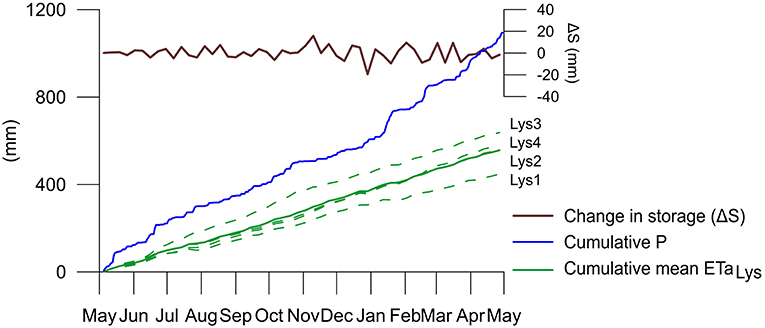
Figure 7. Cumulative evapotranspiration measured with the four lysimeters every 7 days, cumulative precipitation, and the change in soil water storage (ΔS).

Water Balance

Although the water balance method has been extensively used to validate ETa estimates from diverse sources (e.g., remote sensing, models) and three well-monitored microcatchments with different sizes were used in this study to close the water balance, they did not prove to be accurate or to correlate with the EC measurements on a daily timescale. Figure 6 show the mean performance of the three microcatchments depicted in Figure 1. Microcatchments M1–M3 are different in size and relatively similar in terms of vegetation coverage, soil and hydrological properties (see Supplementary Table 1). The M1 microcatchment is the most similar to the EC footprint. Table 4 shows the differences between each microcatchment when comparing their estimates with the EC measurements. The estimates were very similar among microcatchments and only the bias percentage was different. The average was therefore sufficient to give a representation of the performance of the water balance method. However, these estimates did not take into account the change in the soil water storage (ΔS). Figure 8 shows ETa estimates when the ΔS term was included (ETaWB) minus the EC measurements, in comparison with ETa estimates from the water balance when only the precipitation and discharge were used minus the EC measurements. When the ΔS term was included in the water balance through the WCRs measurements, this increased the uncertainties in the estimation of daily ETa. In addition, Table 4 shows the mean estimates of ETa when the term ΔS was considered, confirming its lower performance. This occurred because the WCRs were only located on the supersite hillslope and no other soil VWC measurements were available at Zhurucay. It is noteworthy that the daily over- and under-estimations did not balance one another when they were aggregated weekly or monthly and large differences with EC measurements were still found. However, by the end of the year, the water balance was as accurate as lysimeters in estimating ETa, and was better than the other methods (except PMCal). The concept of closure of the water balance to estimate ETa is the same as the lysimeters' water balance, and when their terms were compared differences arose in the ΔS term. The daily water balance estimates were aggregated to weekly and monthly data, and were found to be far from as good as the lysimeter measurements. At a daily timescale, it is difficult to close the water balance as the precipitation that drains a day after or even later cannot be included. In addition, the poor performance of the water balance could be attributed to the poor estimation of ΔS. This term is important at daily and monthly timescales in order to estimate ETa properly. After 1 year though, the soil water storage is negligible. Studies with long-term data (e.g., Moehrlen et al., 1999; Wilcox et al., 2006; Marc and Robinson, 2007) or with accurate measurements of ΔS (e.g., Wan et al., 2015), have therefore found high accuracy in water balance estimates. However, such studies are uncommon at remote sites (e.g., high altitude sites). Finally, a better measurement of precipitation, which includes hidden precipitation such as drizzle and fog, could close the water balance, and thus ETa could be better estimated.

TABLE 4

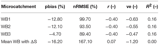
Table 4. Bias percentage (pbias), normalized root mean square error (nRMSE), Pearson's correlation coefficient (r), volumetric efficiency (ve), and coefficient of determination (R²) for the ETa estimates from the water balance closure in three catchments against the eddy-covariance measurements.

FIGURE 8

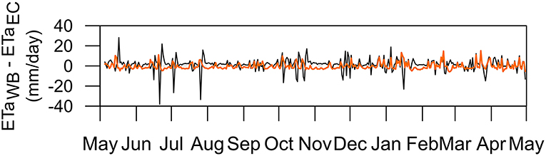
Figure 8. Differences between the mean water balance estimates (without the change in storage term) with EC measurements (orange line) and the differences between the mean water balance estimates (including the change in storage term) and the EC measurements (black line).

Energy Balance

The variables involved in the energy balance were aggregated monthly together with the eddy-covariance measurements in Figure 9, showing their seasonal variance. The net radiation from the eddy-covariance was expected to be smaller than the net radiation from the energy balance, as the measurement elevations differ (3.6 m and 0.6 m, respectively). The ground heat flux was very small and similar between methods. The difference between the ETa estimations with the energy balance and with the EC measurements is therefore attributed to the sensible heat flux estimates. The flux variance method overestimated the sensible heat flux when compared with the EC measurements (Figure 9), therefore the EB method underestimated ETa (Figure 6). The flux variance method is preferred for estimating the sensible heat flux rather than the latent heat flux (Katul et al., 1995; Hsieh et al., 2008), however other studies corroborate that H was overestimated (e.g., Katul et al., 1995). Although the flux variance estimates of H depend on air temperature, wind speed and net radiation (Wesson et al., 2001), we found that for the study site that the estimates' variation is mainly influenced by the air temperature variance (σT), as shown in Figure 9 where the variability between H and σT is the same throughout the year. In the páramo, hourly variations in temperature might be higher than at other sites (σ = 4.5°C/hour), therefore high fluctuations of the H values occur. The energy balance method presented in this study is relatively simple to implement, especially taking into account that G is negligible, and turned out to be more accurate than the water balance method. A more widely used and easy-to-implement method that estimates H or LE is the Bowen ratio-energy balance (BREB) (Fritschen and Simpson, 1989). This method involves differential measurements of temperature and relative humidity, and although it is an indirect measurement of the energy fluxes, it is recommended for future implementation to increase the accuracy of the estimations of ETa with the energy balance methodology.

FIGURE 9

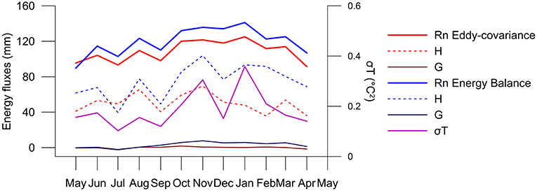
Figure 9. Energy fluxes measured with the eddy-covariance method vs. energy fluxes estimated with the energy balance method. Energy balance method is highly dependent on the variance of the temperature (σT).

The Calibrated Evapotranspiration Equation

After calibration with EC measurements, the coefficients for the ASCE-PM equation were Cn = 550 and Cd = 0.4. They differed from the Penman-Monteith coefficients that estimate ETo (Cn = 900 and Cd = 0.34). Indeed, the ETo and ETa provide different insights, as ETo explains the evapotranspiration when there is no water stress while ETa explains the actual evapotranspiration of the system. The calibration purpose was therefore to find ETa estimates as a function of widely available measurements. The cross-validation of the calibrated evapotranspiration equation proved that results are independent from the dataset (R² = 0.9). The PMCal method is the least biased method (−2%) as EC measurements were used as input for the calibration procedure. Calibration causes a bias correction of the potential evapotranspiration to fit the EC measurements. At our site, this was useful as ETa varies similarly to ETo, as noted in section Actual evapotranspiration and its environmental controls. The differences between PMCal and EC measurements were therefore minimal (Figure 6). Results of the calibrated evapotranspiration equation are accurate and useful at several sites as meteorological stations are widely available. We encourage the use of the calibrated coefficients at páramo sites where only meteorological stations are available to transform the ETo to the ETa estimates, as we have shown here that the common use of ETo to represent evapotranspiration overestimates this important variable by 22%.

The Hydrological Models

The PDM estimates ETa as a function of soil water storage and ETo. In general, model performance was good when compared with the EC measurements (Table 3). The few important differences occurred during November and March (Figure 6). During these months, there was less water available and the PDM underestimated ETa, while the EC measurements showed a relatively high ETa as there was low relative humidity and high ETo that allowed more transpiration (Figure 3). Figure 10 shows the differences between observed field values of VWC and the storage modeled with the PDM (PDM S), which cannot be compared in magnitude but should have the same variability throughout the year. However, it appears that there is no correlation, especially during November and March. Most importantly, the variability was not the same between VWC and PDM S.

FIGURE 10

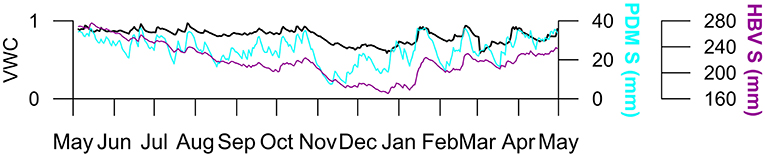
Figure 10. Soil volumetric water content observed with a water content reflectometer (VWC), soil water storage modeled with the PDM (PDM S), and soil water storage modeled with the HBV-light model (HBV S).

The HBV-light model outperformed all methods, evidenced by its high correlation with the EC measurements (0.8–0.9), despite underestimating ETa at the end of the year with a bias of −20%. The bias percentage of the model is higher than other methods, as the over- and under-estimations of the other methods are compensated by the end of the year. HBV-light residuals are small (ranging from −1 to 1) and mostly negative, therefore these underestimations are not compensated, which explains the large negative bias. The volumetric efficiency, on the other hand, analyzes absolute errors, and shows a high performance of the model (ve = 0.8). HBV-light ETa estimates are a function of the same variables as the other models (e.g., PDM). Nevertheless, it appears that the factors multiplying ETo and the soil moisture variables, plus the corrections for temperature anomalies and an estimation of rainfall interception separately from soil evaporation and transpiration (Seibert and Vis, 2012), gave better estimates of ETa. Figure 10 shows the high correlation between VWC and the soil water storage of the HBV-light (HBV S).

It is challenging to represent the change in soil water storage in a model. Even though hydrological models are not very accurate at estimating storage, they take into account this term and this is one important reason why they are well-correlated with daily ETa. Additionally, ETa remains as the only variable that the model needs in order to estimate ETa, as deep percolation and groundwater recharge are negligible at the site. At similar sites where EC or other methods are not available, hydrological models present a solid alternative.

Summary and Conclusions

For the first time, we compared actual evapotranspiration measurements with estimations from several methods in the páramo ecosystem. This study contributes to the advances on the assessment of ETa, which is part of the main challenges established for Earth system science (Fisher et al., 2017). The mean daily actual evapotranspiration was found to be equal to 1.7 mm/day, and in a range from 0.3 to 4 mm/day. Over 1 year, ETa amounted to 622 mm and the ratio of ETa to the total precipitation was 0.57. Furthermore, we have discussed in detail the drivers that led the methods to over- or under-estimate ETa when compared with the EC method. Here we present a brief summary of the suitability of the methods with the main conclusions found in this study.

The main advantages and disadvantages documented for the measurement and estimation of actual evapotranspiration have been summarized in Table 5. In conclusion, the most accurate method with the best temporal resolution is the EC method. However, building the tower includes costly sensors and data corrections that require specific knowledge. A more affordable technique that still gives a complete understanding of the functioning of the environment in terms of the water exchange between the vegetation and the atmosphere, consists in installing the volumetric lysimeters presented here. However, these proved to be effective only when monthly timescales are necessary and when precipitation is accurately measured, taking into account that horizontal precipitation, drizzle and fog are commonly present in the páramo and a disdrometer is preferred over rain gauge measurements (Padrón et al., 2015). The energy balance method also gives a complete understanding of the energy exchange but the sensible heat flux could not be properly estimated in this study and requires further attention.

TABLE 5

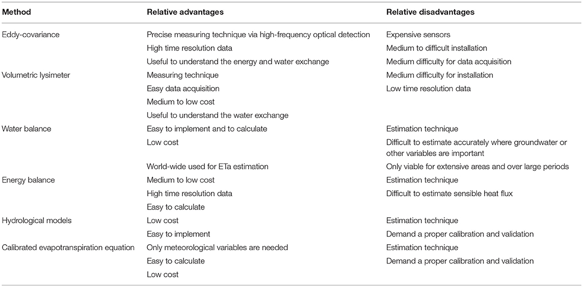
Table 5. General advantages and disadvantages of the actual evapotranspiration measurement and estimation methods.

Although the water balance has been widely used as a validation method for numerous approaches, we have shown here that for relatively small ETa values, the measurement of the change in soil water content plays a crucial role in estimating daily ETa. Even with several WCRs available at our site and information on the soil hydrophysical properties, it was difficult to estimate this term accurately, and at other sites where other variables might be important the accuracy might be even more difficult to improve. Therefore, the water balance is only useful when ETa values are relatively large and other variables are correctly measured or negligible. Furthermore, lysimeters and the water balance method were the least biased in estimating annual ETa, as at the páramo site no other variable appears to be crucial for closing the water balance on that timescale.

When daily estimates and few details on the energy fluxes are needed, the hydrological models (PDM and HBV-light) have proved to be robust for estimating ETa during wet and dry periods. Furthermore, these methods can properly assess the hydrology of the site, are freely available, require only few data as inputs and are easy to implement. They correlate very well with EC measurements and the use of better observations of P (e.g., thorough disdrometers) might improve their accuracy even more.

Finally, it is possible that a meteorological station is available at a páramo site but complete or high-quality data for catchment characterization is not available, and therefore, a model cannot be run. However, the calibration of the Penman-Monteith equation presented here could serve for the estimation of ETa with great accuracy. Moreover, at sites where ETa is not limited by water, the ETo would give very similar results as the ETa. The use of the PM equation is therefore highly advised.

This study has found alternatives to the EC measurements in the páramo grasslands. Further work on this environment is needed to attain higher spatial and temporal resolution. In the future, long-term monitoring studies are required to capture ETa variability under extreme conditions. In addition, partitioning of this variable in the páramo will improve ETa assessment and water resources modeling. These requirements are also important worldwide (Fisher et al., 2017).

Data Availability

The raw data supporting the conclusions of this manuscript will be made available by the authors upon request to any qualified researcher.

Author Contributions

AO-S contributed to installation, maintenance, and data processing of lysimeters, performed data analysis of all methods and wrote the first draft of the manuscript. PC and RC contributed to the conception, design, and supervision of the study, and provided a critical review and editing to the draft of the manuscript. GC-R contributed to installation, maintenance, and data processing of the lysimeters and the eddy-covariance system, and wrote the section on eddy-covariance methodology. AS contributed to the HBV-light modeling. All authors contributed to revision, read and approval of the submitted version of this manuscript.

Conflict of Interest Statement

The authors declare that the research was conducted in the absence of any commercial or financial relationships that could be construed as a potential conflict of interest.

Acknowledgments

This work was funded by the Research Office of the University of Cuenca (DIUC) through the Project XIII–Conc: Estudio Comparativo de Métodos de Estimación de Evapotranspiración Actual en Suelos Húmedos de una Micro cuenca de Páramo Andino and by the Ecuadorian Secretary of Higher Education, Science, Technology and Innovation (SENESCYT) through Programa de Fortalecimiento de las Capacidades en Ciencia, Tecnología, Investigación e Innovación de las Instituciones de Educación Superior Públicas (2013–2014). We thank these institutions for providing generous funding. We also thank Comuna Chumblín Sombrederas (Azuay, San Fernando) and INV Metals (Canada), Project Loma Larga-Ecuador, for providing logistical support. This manuscript is an outcome of the Doctoral Program in Water Resources, offered by Universidad de Cuenca, Escuela Politécnica Nacional, and Universidad Técnica Particular de Loja. The first author gratefully acknowledges University of Cuenca for funding her PhD scholarship.

Supplementary Material

The Supplementary Material for this article can be found online at: https://www.frontiersin.org/articles/10.3389/feart.2019.00055/full#supplementary-material

References

Baldocchi, D. D. (2003). Assessing the eddy covariance technique for evaluating carbon dioxide exchange rates of ecosystems: past, present and future. Glob. Chang. Biol. 9, 479–492. doi: 10.1046/j.1365-2486.2003.00629.x

CrossRef Full Text | Google Scholar

Bergström, S. (1976). Development and Application of a Conceptual Runoff Model for Scandinavian Catchments. Norrköpin: Swedish Meteorological and Hydrological Institute.

Google Scholar

Boll, J., Steenhuis, T. S., and Selker, J. S. (1992). Fiberglass wicks for sampling of water and solutes in the vadose zone. Soil Sci. Soc. Am. J. 56, 701–707. doi: 10.2136/sssaj1992.03615995005600030005x

CrossRef Full Text | Google Scholar

Bowden, W. B., Fahey, B. D., Ekanayake, J., and Murray, D. L. (2001). Hillslope and wetland hydrodynamics in a tussock grassland, South Island, New Zealand. Hydrol. Process 15, 1707–1730. doi: 10.1002/hyp.235

CrossRef Full Text | Google Scholar

Cabral, O. M. R., da Rocha, H. R., Gash, J. H., Freitas, H. C., and Ligo, M. A. V. (2015). Water and energy fluxes from a woodland savanna (cerrado) in southeast Brazil. J. Hydrol. Reg. Stud. 4, 22–40. doi: 10.1016/j.ejrh.2015.04.010

CrossRef Full Text | Google Scholar

Cabral, O. M. R., Rocha, H. R., Gash, J. H. C., Ligo, M. A. V., Freitas, H. C., and Tatsch, J. D. (2010). The energy and water balance of a Eucalyptus plantation in southeast Brazil. 338, 208–216. J. Hydrol. doi: 10.1016/j.jhydrol.2010.04.041

CrossRef Full Text | Google Scholar

Campbell, D. I., and Murray, D. L. (1990). Water balance of snow tussock grassland in New Zealand. J. Hydrol. 118, 229–245. doi: 10.1016/0022-1694(90)90260-5

CrossRef Full Text | Google Scholar

Carrillo-Rojas, G., Silva, B., Córdova, M., Célleri, R., and Bendix, J. (2016). Dynamic mapping of evapotranspiration using an energy balance-based model over an andean páramo catchment of southern ecuador. Remote Sens. 8:160. doi: 10.3390/rs8020160

CrossRef Full Text | Google Scholar

Carrillo-Rojas, G., Silva, B., Rollenbeck, R., Célleri, R., and Bendix, J. (2019). The breathing of the Andean highlands: net ecosystem exchange and evapotranspiration over the páramo of southern Ecuador. Agric. For. Meteorol. 265, 30–47. doi: 10.1016/j.agrformet.2018.11.006

CrossRef Full Text | Google Scholar

Clark, K. E., Torres, M. A., West, A. J., Hilton, R. G., New, M., Horwath, A. B., et al. (2014). The hydrological regime of a forested tropical Andean catchment. Hydrol. Earth Syst. Sci. 18, 5377–5397. doi: 10.5194/hess-18-5377-2014

CrossRef Full Text | Google Scholar

Coners, H., Babel, W., Willinghöfer, S., Biermann, T., Köhler, L., Seeber, E., et al. (2016). Evapotranspiration and water balance of high-elevation grassland on the Tibetan Plateau. J. Hydrol. 533, 557–566. doi: 10.1016/j.jhydrol.2015.12.021

CrossRef Full Text | Google Scholar

Córdova, M., Carrillo-Rojas, G., and Célleri, R. (2013). Errores en la estimacion de la evapotranspiracion de referencia de una zna de paramo andino debido al uso de datos mensuales, diarios y horarios. Aqua-LAC 5, 14–22. Available online at: http://www.unesco.org/new/es/office-in-montevideo/natural-sciences/water-ihp-lac/revista-aqualac/aqua-lac-10-2013/

Córdova, M., Carrillo-Rojas, G., Crespo, P., Wilcox, B., and Célleri, R. (2015). Evaluation of the penman-monteith (FAO 56 PM) method for calculating reference evapotranspiration using limited data. Mt. Res. Dev. 35, 230–239. doi: 10.1659/MRD-JOURNAL-D-14-0024.1

CrossRef Full Text | Google Scholar

Criss, R. E., and Winston, W. E. (2008). Do Nash values have value? Discussion and alternate proposals. Hydrol. Process 22, 2723–2725. doi: 10.1002/hyp.7072

CrossRef Full Text | Google Scholar

Falge, E., Baldocchi, D., Olson, R., Anthoni, P., Aubinet, M., Bernhofer, C., et al. (2001). Gap filling strategies for defensible annual sums of net ecosystem exchange. Agric. For. Meteorol. 107, 43–69. doi: 10.1016/S0168-1923(00)00225-2

CrossRef Full Text | Google Scholar

Fisher, J. B., Malhi, Y., Bonal, D., Da Rocha, H. R., De Araújo, A. C., Gamo, M., et al. (2009). The land-atmosphere water flux in the tropics. Glob. Chang. Biol. 15, 2694–2714. doi: 10.1111/j.1365-2486.2008.01813.x

CrossRef Full Text | Google Scholar

Fisher, J. B., Melton, F., Middleton, E., Hain, C., Anderson, M., Allen, R., et al. (2017). The future of evapotranspiration: global requirements for ecosystem functioning, carbon and climate feedbacks, agricultural management, and water resources. Water Resour. Res. 53, 2618–2626. doi: 10.1002/2016WR020175

CrossRef Full Text | Google Scholar

Foley, J. A., Ramankutty, N., Brauman, K. A., Cassidy, E. S., Gerber, J. S., Johnston, M., et al. (2011). Solutions for a cultivated planet. Nature 478, 337–342. doi: 10.1038/nature10452

PubMed Abstract | CrossRef Full Text | Google Scholar

Fritschen, L. J., and Simpson, J. R. (1989). Surface energy and radiation balance systems: general description and improvements. J. Appl. Meteorol. Climatol. 28, 680–689. doi: 10.1175/1520-0450(1989)028<0680:SEARBS>2.0.CO;2

CrossRef Full Text | Google Scholar

Gebler, S., Hendricks Franssen, H. J., Pütz, T., Post, H., Schmidt, M., and Vereecken, H. (2015). Actual evapotranspiration and precipitation measured by lysimeters: a comparison with eddy covariance and tipping bucket. Hydrol. Earth Syst. Sci. 19, 2145–2161. doi: 10.5194/hess-19-2145-2015

CrossRef Full Text | Google Scholar

Gu, S., Tang, Y., Cui, X., Du, M., Zhao, L., Li, Y., et al. (2008). Characterizing evapotranspiration over a meadow ecosystem on the Qinghai-Tibetan Plateau. J. Geophys. Res. Atmos. 113:D08118. doi: 10.1029/2007JD009173

CrossRef Full Text | Google Scholar

Hofstede, R., Calles, J., López, V., Polanco, R., Torres, F., Ulloa, J., et al. (2014). Los páramos Andinos ¿Qué Sabemos? Estado de conocimiento sobre el impacto del cambio climático en el ecosistema páramo. IUCN. Quito, Ecuador.

Holdsworth, D. K., and Mark, A. F. (1990). Water and nutrient input:output budgets: effects of plant cover at seven sites in upland snow tussock grasslands of eastern and central Otago, New Zealand. J. R. Soc. New N. Zeal. 20, 1–24. doi: 10.1080/03036758.1990.10426730

CrossRef Full Text | Google Scholar

Hsieh, C. I., Lai, M. C., Hsia, Y. J., and Chang, T. J. (2008). Estimation of sensible heat, water vapor, and CO2 fluxes using the flux-variance method. Int. J. Biometeorol. 52, 521–533. doi: 10.1007/s00484-008-0149-4

PubMed Abstract | CrossRef Full Text | Google Scholar

Iniguez, V., Morales, O., Cisneros, F., Bauwens, W., and Wyseure, G. (2016). Analysis of the drought recovery of Andosols on southern Ecuadorian Andean paramos. Hydrol. Earth Syst. Sci. 20, 2421–2435. doi: 10.5194/hess-20-2421-2016

CrossRef Full Text | Google Scholar

Jones, P. D., and Hulme, M. (1996). Calculating regional climatic time series for temperature and precipitation: methods and illustrations. Int. J. Climatol. 16, 361–377. doi: 10.1002/(SICI)1097-0088(199604)16:4<361::AID-JOC53>3.0.CO;2-F

CrossRef Full Text | Google Scholar

Katul, G., Goltz, S. M., Hsieh, C. I., Cheng, Y., Mowry, F., and Sigmon, J. (1995). Estimation of surface heat and momentum fluxes using the flux-variance method above uniform and non-uniform terrain. Bound. Layer Meteorol. 74, 237–260. doi: 10.1007/BF00712120

CrossRef Full Text | Google Scholar

Khan, B. R., Mainuddin, M., and Molla, M. N. (1993). Design, construction and testing of a lysimeter for a study of evapotranspiration of different crops. Agric. Water Manag. 23, 183–197. doi: 10.1016/0378-3774(93)90027-8

CrossRef Full Text | Google Scholar

Kljun, N., Calanca, P., Rotach, M. W., and Schmid, H. P. (2015). A simple two-dimensional parameterisation for Flux Footprint Prediction (FFP). Geosci. Model Dev. 8, 3695–3713. doi: 10.5194/gmd-8-3695-2015

CrossRef Full Text | Google Scholar

Knowles, J. F., Burns, S. P., Blanken, P. D., and Monson, R. K. (2015). Fluxes of energy, water, and carbon dioxide from mountain ecosystems at Niwot Ridge, Colorado. Plant Ecol. Divers. 8, 663–676. doi: 10.1080/17550874.2014.904950

CrossRef Full Text | Google Scholar

Llambí, L. D., Soto, -W. A., Célleri, R., Bièvre, B., De O.choa, B., and Borja, P. (2012). Ecología, Hidrología y Suelos de Páramos, Lima: Proyecto Páramo Andino.

Marc, V., and Robinson, M. (2007). The long-term water balance (1972-2004) of upland forestry and grassland at Plynlimon, mid-Wales. Hydrol. Earth Syst. Sci. 11, 44–60. doi: 10.5194/hess-11-44-2007

CrossRef Full Text | Google Scholar

Mauder, M., Cuntz, M., Drüe, C., Graf, A., Rebmann, C., Schmid, H. P., et al. (2013). A strategy for quality and uncertainty assessment of long-term eddy-covariance measurements. Agric. For. Meteorol. 169, 122–135. doi: 10.1016/j.agrformet.2012.09.006

CrossRef Full Text | Google Scholar

Mayocchi, C. L., and Bristow, K. L. (1995). Soil surface heat flux: some general questions and comments on measurements. Agric. For. Meteorol. 75, 43–50. doi: 10.1016/0168-1923(94)02198-S

CrossRef Full Text | Google Scholar

Moehrlen, C., Kiely, G., and Pahlow, M. (1999). Long term water budget in a grassland catchment in Ireland. Phys. Chem. Earth Part B Hydrol. Ocean. Atmos. 24, 23–29. doi: 10.1016/S1464-1909(98)00006-9

CrossRef Full Text | Google Scholar

Monson, R., and Baldocchi, D. (2014). Terrestrial Biosphere-Atmosphere Fluxes. Cambridge: Cambridge University Press. doi: 10.1017/CBO9781139629218

CrossRef Full Text | Google Scholar

Moore, R. J. (1985). The probability-distributed principle and runoff production at point and basin scales. Hydrol. Sci. J. 30, 273–297. doi: 10.1080/02626668509490989

CrossRef Full Text | Google Scholar

Moore, R. J., and Clarke, R. T. (1981). A distribution function approach to rainfall runoff modeling. Water Resour. Res. 13, 1367–1382. doi: 10.1029/WR017i005p01367

CrossRef Full Text | Google Scholar

Novick, K., Brantley, S., Miniat, C. F., Walker, J., and Vose, J. M. (2014). Inferring the contribution of advection to total ecosystem scalar fluxes over a tall forest in complex terrain. Agric. For. Meteorol. 185, 1–13. doi: 10.1016/j.agrformet.2013.10.010

CrossRef Full Text | Google Scholar

Ochoa-Sánchez, A., Crespo, P., and Célleri, R. (2018). Quantification of rainfall interception in the high Andean tussock grasslands. Ecohydrology 11:e1946. doi: 10.1002/eco.1946

CrossRef Full Text | Google Scholar

Ochoa-Tocachi, B. F., Buytaert, W., Antiporta, J., Acosta, L., Bardales, J. D., Célleri, R., et al. (2018). High-resolution hydrometeorological data from a network of headwater catchments in the tropical Andes. Sci. Data 5:180080. doi: 10.1038/sdata.2018.80

PubMed Abstract | CrossRef Full Text | Google Scholar

Oki, T., and Kanae, S. (2006). Global hydrological cycles and world water resources. Science 313, 1068–1072. doi: 10.1126/science.1128845

PubMed Abstract | CrossRef Full Text | Google Scholar

Padrón, R. S., Wilcox, B. P., Crespo, P., and Célleri, R. (2015). Rainfall in the andean páramo: new insights from high-resolution monitoring in southern ecuador. J. Hydrometeorol. 16, 985–996. doi: 10.1175/JHM-D-14-0135.1

CrossRef Full Text | Google Scholar

Papale, D., Reichstein, M., Aubinet, M., Canfora, E., Bernhofer, C., Kutsch, W., et al. (2006). Towards a standardized processing of Net Ecosystem Exchange measured with eddy covariance technique: algorithms and uncertainty estimation. Biogeosciences 3, 571–583. doi: 10.5194/bg-3-571-2006

CrossRef Full Text | Google Scholar

Poss, J. A., Russell, W. B., Shouse, P. J., Austin, R. S., Grattan, S. R., Grieve, C. M., et al. (2004). A volumetric lysimeter system (VLS): an alternative to weighing lysimeters for plant-water relations studies. Comput. Electron. Agric. 43, 55–68. doi: 10.1016/j.compag.2003.10.001

CrossRef Full Text | Google Scholar

Rana, G., and Katerji, N. (2000). Measurement and estimation of actual evapotranspiration in the field under Mediterranean climate: a review. Eur. J. Agron. 13, 125–153. doi: 10.1016/S1161-0301(00)00070-8

CrossRef Full Text | Google Scholar

Reichstein, M., Falge, E., Baldocchi, D., Papale, D., Aubinet, M., Berbigier, P., et al. (2005). On the separation of net ecosystem exchange into assimilation and ecosystem respiration: review and improved algorithm. Glob. Chang. Biol. 11, 1424–1439. doi: 10.1111/j.1365-2486.2005.001002.x

CrossRef Full Text | Google Scholar

Rose, C. W., and Sharma, M. L. (1984). Summary and recommendations of the Workshop on Evapotranspiration from plant communities. Agric. Water Manag. 8, 325–342. doi: 10.1016/0378-3774(84)90061-1

CrossRef Full Text | Google Scholar

Seibert, J., and Vis, M. J. P. (2012). Teaching hydrological modeling with a user-friendly catchment-runoff-model software package. Hydrol. Earth Syst. Sci. 16, 3315–3325. doi: 10.5194/hess-16-3315-2012

CrossRef Full Text | Google Scholar

Serrano-Ortiz, P., Sánchez-Cañete, E. P., Olmo, F. J., Metzger, S., Pérez-Priego, O., Carrara, A., et al. (2016). Surface-parallel sensor orientation for assessing energy balance components on mountain slopes. Bound. Layer Meteorol. 158, 489–499. doi: 10.1007/s10546-015-0099-4

CrossRef Full Text | Google Scholar

Sucozhañay, A., and Célleri, R. (2018). Impact of rain gauges distribution on the runoff simulation of a small mountain catchment in southern ecuador. Water 10:1169. doi: 10.3390/w10091169

CrossRef Full Text | Google Scholar

van den Bergh, T., Inauen, N., Hiltbrunner, E., and Körner, C. (2013). Climate and plant cover co-determine the elevational reduction in evapotranspiration in the Swiss Alps. J. Hydrol. 500, 75–83. doi: 10.1016/j.jhydrol.2013.07.013

CrossRef Full Text | Google Scholar

Wagener, T., Boyle, D. P., Lees, M. J., Wheater, H. S., Gupta, H. V., and Sorooshian, S. (2001). A framework for development and application of hydrological models. Hydrol. Earth Syst. Sci. 5, 13–26. doi: 10.5194/hess-5-13-2001

CrossRef Full Text | Google Scholar

Walter, I. A., Allen, R. G., Elliott, R., Jensen, M. E., Itenfisu, D., Mecham, B., et al. (2000). “ASCE's standardized reference evapotranspiration equation,” in Watershed Management and Operations Management 2000. Task Committee on Standardization of Reference Evapotranspiration and the Water Management Committee of the Irrigation Association. 10.

Google Scholar

Wan, Z., Zhang, K., Xue, X., Hong, Z., Hong, Y., and Gourley, J. J. (2015). Water balance-based actual evapotranspiration reconstruction from ground and satellite observations over the conterminous United States. Water Resour. Res. 51, 6485–6499. doi: 10.1002/2015WR017311

CrossRef Full Text | Google Scholar

Wesson, K. H., Katul, G., and Lai, C. -T. (2001). Sensible heat flux estimation by flux variance and half-order time derivative methods. Water Resour. Res. 37, 2333–2343. doi: 10.1029/2001WR900021

CrossRef Full Text | Google Scholar

Wilcox, B. P., Dowhower, S. L., Teague, W. R., and Thurow, T. L. (2006). Long-term water balance in a semiarid shrubland. Rangel. Ecol. Manag. 59, 600–606. doi: 10.2111/06-014R3.1

CrossRef Full Text | Google Scholar