 Richard Hoffmann
 Alain Dassargues
 Pascal Goderniaux2
 Thomas Hermans
- 1Hydrogeology and Environmental Geology, GEO3, UEE, Liège University, Liege, Belgium
- 2Geology and Applied Geology, Polytech Mons, University of Mons, Mons, Belgium
- 3Department of Geology, Ghent University, Ghent, Belgium
In heterogeneous aquifers, imaging preferential flow paths, and non-Gaussian effects is critical to reduce uncertainties in transport predictions. Common deterministic approaches relying on a single model for transport prediction show limitations in capturing these processes and tend to smooth parameter distributions. Monte-Carlo simulations give one possible way to explore the uncertainty range of parameter value distributions needed for realistic predictions. Joint heat and solute tracer tests provide an innovative option for transport characterization using complementary tracer behaviors. Heat tracing adds the effect of heat advection-conduction to solute advection-dispersion. In this contribution, a joint interpretation of heat and solute tracer data sets is proposed for the alluvial aquifer of the Meuse River at the Hermalle-sous-Argenteau test site (Belgium). First, a density-viscosity dependent flow-transport model is developed and induce, due to the water viscosity changes, up to 25% change in simulated heat tracer peak times. Second, stochastic simulations with hydraulic conductivity (K) random fields are used for a global sensitivity analysis. The latter highlights the influence of spatial parameter uncertainty on the resulting breakthrough curves, stressing the need for a more realistic uncertainty quantification. This global sensitivity analysis in conjunction with principal component analysis assists to investigate the link between the prior distribution of parameters and the complexity of the measured data set. It allows to detect approximations done by using classical inversion approaches and the need to consider realistic K-distributions. Furthermore, heat tracer transport is shown as significantly less sensitive to porosity compared to solute transport. Most proposed models are, nevertheless, not able to simultaneously simulate the complementary heat-solute tracers. Therefore, constraining the model using different observed tracer behaviors necessarily comes with the requirement to use more-advanced parameterization and more realistic spatial distribution of hydrogeological parameters. The added value of data from both tracer signals is highlighted, and their complementary behavior in conjunction with advanced model/prediction approaches shows a strong uncertainty reduction potential.
Introduction and Motivation
Heterogeneity in porous media, inducing preferential flow paths, and non-Gaussian effects, influences significantly subsurface transport (among others: Fuchs et al., 2009; Heeren et al., 2010). An improved imaging of these preferential pathways, in connection with reducing uncertainty in transport simulations and predictions, is crucial for answering future groundwater quality questions.
Innovative tracer test set-ups, along with relevant interpretations, are possible new ways for quantifying more realistically this heterogeneity and the associated uncertainty (Davis et al., 1980; Maliva, 2016). In this context, heat is considered as a complementary tracer, compared to conservative solute tracers (saline tracer or fluorescent dye). Heat is usually considered as a non-conservative tracer, allows information about advection-conduction processes to be obtained, and heat has a natural retardation and more diffusion linked to the heat capacity of the solid (Anderson, 2005). Using both, solute and heat, thus provides two tracer plumes that can be compared, allows more information about the solid matrix properties to be obtained, and enables the quantification of subsurface processes (immobile water, matrix contributions) with a better resolution (Anderson, 2005; Irvine et al., 2015). For example, Wildemeersch et al. (2014) combine heat and solute tracer experiments to assess the heterogeneity in an alluvial aquifer. Sarris et al. (2018) also give a recent application of jointly interpreting heat and solute tracer data. They show, in a deterministic way, how these innovative tracer tests can contribute to a high-resolution description of deposits, and a significant improvement of transport processes understanding. In the joint heat and solute tracer inversion by Sarris et al. (2018), heat and solute seem to be sensitive to hydraulic conductivity and porosity. In their case study, heat also shows a stronger sensitivity to vertical hydraulic conductivity, resulting in a more complex aquifer parametrization, and more realistic transport predictions.
Deterministic approaches are useful for process understanding. However, predictions based on an unique “best” model parametrization bear a lot of uncertainty and, thus, must be justified and used with care (Renard, 2007; Remonti and Mori, 2016). Deterministic approaches generally reduce heterogeneity, typically by replacing spatially distributed properties by averaged properties, leading to poorer predictions with underestimated uncertainty (Alcolea et al., 2006; Renard, 2007). Using additional information gained from joint heat and solute tracer tests adds more constraints to the inversion process. However, when the tracer behavior is getting more complex, deterministic approaches can quickly turn into ill-posed inverse problems (Zhou et al., 2014), reducing their predictive reliability. Classical deterministic inversion approaches could therefore be questioned.
To explain and adequately represent the observed variables, more advanced transport simulation and forecast approaches, such as stochastic methods (Ptak et al., 2004), are generally required. Monte-Carlo simulations may, for example, be used to explore uncertainty ranges and to consider heterogeneity (among others, Ptak et al., 2004; Renard, 2007, Ferré, 2017). However, the full stochastic inversion of hydrogeological data when spatial uncertainty plays a key role remains difficult and time consuming, limiting the applicability of the methods (Renard, 2007). In this context, transdimensional inference (e.g., Sambridge et al., 2012) is a possible approach to combine the parsimony principle with stochastic inversion. In practice, transdimensional inference includes the number of parameters as an unknown, and therefore limits the complexity of the model to what is necessary to explain the data.
However, if field data is sparse and prior uncertainty is large, the transdimensional approach would also lead to an oversimplification of the model, which can be harmful for its predictive capability (referred to Hermans (2017), about the importance of realistic consideration of prior uncertainty). In contrast, a full stochastic approach allows realistically quantifying the uncertainty for transport predictions, instead of having a single deterministic inversion or multiple simulations with (partly) non-quantified approximations (among others, Caers, 2011; Hermans, 2017; Hermans et al., 2018; Scheidt et al., 2018). In combination with the use of complementary tracers such as heat, stochastic approaches and data analysis methods have a strong potential to learn more from collected data sets and falsify approximations done in conceptual models and prior estimations (Hermans et al., 2015a,b, 2016, 2018).
A further new potential for hydrogeological applications and transport predictions is Bayesian Evidential Learning (BEL) (Hermans, 2017; Hermans et al., 2018; Scheidt et al., 2018). BEL relies on a limited number of Monte-Carlo simulations sampling the prior distribution of model parameters, in order to analyze the global sensitivity of parameters (Park et al., 2016; Hermans et al., 2018) and falsify the prior distribution. In comparison to common single parameter sensitivity analysis, regionalized or global sensitivity analyses consider heterogenous sources of model uncertainty (e.g., Park et al., 2016). The falsification step consists in obtaining consistency between the sampled simulation data (i.e., prior) and the reference data (Hermans et al., 2015a; Scheidt et al., 2018). BEL can also be used, if necessary, to identify a statistical relationship between historical and forecast variables (Hermans, 2017; Hermans et al., 2018; Scheidt et al., 2018). The common inversion step is thus replaced by finding the direct relationship between the prior (sampled simulation data) and the desired forecast, which only depends on the complexity of the subsurface (i.e., model) (Hermans, 2017). Using Monte-Carlo, samples from the prior distribution are generated and used to simultaneously simulate synthetic data and forecasts. Both outcomes are analyzed for detecting direct relationships. Following this innovative approach, cost-expensive inversion can be avoided by reformulating the prediction problem, and the likelihood directly in terms of the forecast (Hermans, 2017).
For addressing the uncertainty of transport predictions, for instance due to preferential flow paths, any forecasting approach should first consider realistic parameter uncertainty related to heterogeneity. In this paper and the context of BEL, “prior” is defined as the prior distribution of model parameters, according to the current knowledge of the field, and from which outcome samples are randomly drawn in Monte-Carlo methods (Rojas et al., 2009; Caers, 2011; Hermans, 2017).
In this paper, the prior uncertainty is investigated for a heterogeneous alluvial aquifer, using joint heat and solute tracer data, through a global sensitivity analysis. A performed tracer experiment (Wildemeersch et al., 2014; Hermans et al., 2015b) has been previously used by Klepikova et al. (2016), to calibrate a deterministic model through automatic inversion. The HydroGeoSphere code (HGS) was used allowing full 3D simulations (Therrien et al., 2010; Brunner and Simmons, 2012). HGS was used in conjunction with PEST as a parameter estimation tool for inversion (Doherty, 1994, 2003). Although those first analyses helped to understand groundwater flow and solute and heat transport in the aquifer, they also showed that the approximations impeded to explain simultaneously all observations. In Hermans et al. (2015a, 2018), additional stochastic approaches considering spatial uncertainty were successfully used in explaining parts of the experimental data, but they considered only limited data sets or parts of the whole aquifer system. In this paper, the current conceptual approximations (the prior) in the description of the alluvial deposits will be revisited with the goal to improve the heterogeneity characterization. Generating a prior, consistent with the observed heat and solute tracer test data, is a necessary step to being able to realistically predict transport in this complex geological setting.
Within this context, the objective of the paper is to take advantage of the complementary behavior of heat and solute tracers to better characterize the heterogeneity in the aquifer system. The aim is to formulate a more realistic prior and analyze its consistency, before moving toward more advanced prior analysis and direct predictions using the BEL framework. For this purpose, the variability of the tracer output signals will be analyzed (1) through a deterministic model, and (2) using Monte-Carlo simulations, followed by a global sensitivity analysis.
Materials and Methods
Test Site: Hermalle-Sous-Argenteau
The test site of Hermalle-sous-Argenteau (HssA) in the north of Liege (Belgium) lies between the canal Albert and the Meuse River (Figure 1A) in an alluvial plain field with a groundwater natural gradient of around 0.06 %. Between the 20 m distant injection well (Pz09) and the pumping well (PP), there are three panels with 10 piezometers including 19 observation points (i.e., most piezometers are screened at two different levels, Figure 1B). The first panel is located at 3 m, the second at 8 m and the third at 15 m from the injection well. An evaluation of the borehole logs during drilling shows that the aquifer is mostly composed of sandy gravel. The sand matrix is finer in the top part and its proportion decreases in the bottom part (Figure 1B). In previous studies, the adopted conceptual model split the aquifer in two layers, an upper (K = 2.38·10−3 m s−1) and a lower (K = 4.67·10−2 m s−1) part (Klepikova et al., 2016; Hermans et al., 2018). The estimated bulk thermal conductivity is in the range κb = 1.37 W m−1 K−1 to 1.86 W m−1 K−1 (Klepikova et al., 2016).
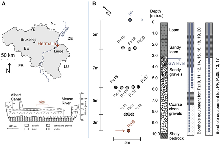
Figure 1. (A) Overview of the field site location. (B) Borehole location showing the three panels between the injection well (Pz9) and the pumping well (PP), a typical log, and borehole equipment [modified figure according to Wildemeersch et al. (2014)].
The reference data set used in this study was described in Wildemeersch et al. (2014). A joint heat and solute tracer experiment was performed with a 24 h and 20 min continuous injection of heat (ΔT = 25.5 K) and naphtionate (C = 5.48 mg L−1) at the rate of 3 m3 h−1, while 30 m3 h−1 were extracted from the pumping well PP. Temperature distribution was the focus and therefore measured in all observation points, while the solute tracer was only measured in PP for validation purposes. Measurements in Pz13 and Pz17 are not used because these observation wells are uniformly screened all over the aquifer and do not allow separated measurements in both the upper and lower compartments (Klepikova et al., 2016; Hermans et al., 2018).
The observed heat tracer plume shows that the heat injected in the lower aquifer part tends to move upwards very quickly toward the first panel, then to be split and move downwards (Wildemeersch et al., 2014). The measured temperature in the second upper panel is significantly lower than in the first upper panel (for detailed measured reference data at all panels, we refer to the “Supplementary Material Figures 1–4”). This observed behavior is currently difficult to be simulated for all observation locations with just one deterministic model inverted with common methods, e.g., using pilot points (Klepikova et al., 2016).
Deterministic Porous Media Model
Based on the current conceptual two-layer aquifer model (each 3.5 m thick), Klepikova et al. (2016) developed a numerical model focusing on the heat transport simulation using HGS in finite difference mode (Therrien et al., 2010) and a pilot point approach (Doherty, 2003) to calibrate the model against heat data. This model is density dependent during the first 24 h only, as density effects were expected to be low afterwards (Ma and Zheng, 2009; Klepikova et al., 2016). This model describes a 40 × 60 × 7 m volume of alluvial aquifer with a grid of 84,280 elements in total. No recharge was assumed for the duration of the experiment. Due to the high permeability of the gravel, the vertical leakage at the bottom of the model was considered as negligible compared to lateral input/output. The initial groundwater temperature was set to Tini = 13.48 °C according to the measured values before the experiment. The model was running under transient flow conditions due to the simulation of the tracer experiment. Peclet numbers of 300 for the upper part, and 14,000 for the lower part were computed, suggesting an expected advection-dominated transport (Klepikova et al., 2016).
Here, this model is extended with a simultaneous solute injection. In HGS, the injection is simulated selecting two nodes next to each other: at the first node, representing the screen location in the borehole, the solute tracer is injected and one node below the heat is injected, respecting the actual experimental set-up. Both injections are simulated using Neumann (2nd type) boundary conditions. For the solute injection, the prescribed mass injection rate is 4.3 10−6kg s−1. For the heat injection, the prescribed injection rate is 8.3·10−4 J K−1 s−1 (Klepikova et al., 2016). The grid is refined to 140,140 rectangular elements with 14 numerical grid sublayers (each 0.5 m thick), allowing a better representation of the spatial heterogeneity and uncertainty. To account for the influence of immobile water on heat conduction, an apparent thermal conductivity is computed using:
θ is the total porosity with 0.12, neff the effective porosity with 0.05, or otherwise called mobile water porosity, κf the fluid thermal conductivity with 0.59 W m−1 K−1 and κs the solid thermal conductivity estimated from previous works to around 1.43 W m−1 K−1. As temperature affects the groundwater density and dynamic viscosity, the injected heat influences both groundwater flow and transport simulations. In contrast to Klepikova et al. (2016), the new numerical implementation allows fully density-dependent, but also viscosity-dependent simulations.
Stochastic Prior Uncertainty Investigation
This study investigates the prior-uncertainty using Monte-Carlo simulations, followed by a global sensitivity analysis and prior falsification. The applied procedure in this study corresponds to the first, second and third steps of the BEL method as described by Hermans et al. (2018). In the Monte-Carlo simulations, part of the calibrated values from the deterministic model parameters are replaced by random values sampled from random uniform distributions (Table 1).
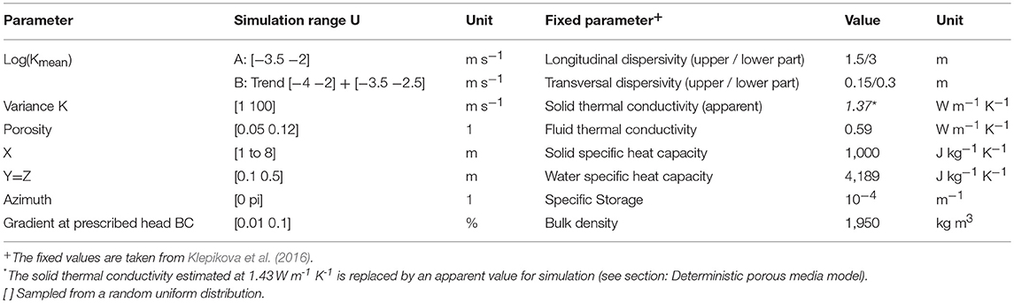
Table 1. Parameter simulation ranges for the Monte-Carlo simulations (left column) and chosen fixed parameter values identical to those chosen by Klepikova et al. (2016) (right column).
In each Monte-Carlo simulation step (prior sampling), a new HGS forward model is parameterized with randomly generated advection global parameters, like the log(Kmean), the K variance, the porosity, the variogram ranges in X,Y,Z directions, the azimuth, and the gradient between the two main prescribed head boundary conditions located upgradient from the injection well and downgradient from the pumping well. Fixed values [i.e., identical to those chosen by Klepikova et al. (2016)] are considered for dispersivity, thermal conductivity, specific heat capacity, specific storage, and bulk density (Table 1). To represent the K-distribution within each Monte-Carlo simulation more realistically, sequential Gaussian simulations are used following two scenarios.
Scenario A uses the prior distribution from Hermans et al. (2015a). This prior was not falsified by geophysical and hydrogeological data acquired during the experiment (Hermans et al., 2015a) in the middle panel. It was thus not tested against the whole available data set, as it is proposed here. In particular, it uses the same two-layer approximation and ignores any trend in the alluvial deposits grain size distribution. Random Kmean values between 10−3.5 and 10−2.5 m s−1 in conjunction with a K-variance between 1 and 100 m s−1 are considered. Models are randomly generated without any additional constraint.
Scenario B considers the trend observed during drilling (Figure 1B) in the alluvial deposits, in which it is assumed that grain size distributions influenced the hydraulic conductivity values. Within 14 constrained sublayers, a vertical downwards increasing K-trend is considered in the geostatistical simulations. Within every Monte-Carlo step, for the 12 sublayers between the fixed top (Kmean = 10−4 m s−1) and bottom (Kmean = 10−2 m s−1) sublayer, new random generated mean values between Kmean = 10−3.5 and 10−2.5 m s−1, increasing downwards, are used. To account for field observations (see section Test site: Hermalle-sous-Argenteau, Wildemeersch et al., 2014; Hermans et al., 2015b) showing that the heat plume does not follow a straight path toward the pumping well, the possible occurrence of local low hydraulic conductivity zones (flow barriers) in the aquifer is thus considered. The presence of loam lenses with low hydraulic conductivity are actually observed at some places in the Meuse river alluvial deposits and are here assumed as a possible origin/explanation for the observed behavior. Two flow barriers are placed in front of Pz14 and Pz17 in the upper part, and the third one in the lower aquifer part between the injection well and Pz11. The constrained hydraulic conductivity is four orders of magnitude lower. Within the sequential Gaussian simulation, the fixed constrained K-values are considered as hard data for the random simulations. The size of the potential flow barriers is thus dependent on variogram characteristics.
For each scenario, 250 simulations are generated through Monte-Carlo methods. This number was considered sufficient to model the variability in the prior data sets, while keeping the computational cost to a minimum, and to estimate the global sensitivity analysis (see below). The reason lies in the fact that the used approach analyzes the data response (temperature or solute curve) which is less complex than the model spatial heterogeneity, therefore requiring only a limited number of samples (Hermans et al., 2018).
A distance metric using the root of the square sums of the difference between each simulated f(ti) and observed g(ti) data over the same experimental time interval tExp (0–10 days), showing positive zero definition, symmetry, and triangle inequality, is used to compare the ability of different simulations to reproduce field data. It allows to identify the best realization at each observation point within the generated 250 realizations, separately for each scenario:
Best simulation at observation point means minimizing:
Best simulations are quantified calculating the root mean square error (RMSE) and the correlation coefficient (R2).
Distance Based Sensitivity Analysis
A global sensitivity analysis reveals key information about model parameters most influencing the simulated data at observation points. With the output signals of the heat and solute realizations, the distance-based global sensitivity analysis (DGSA, Park et al., 2016) is applied, considering the global and spatial parameters of each simulation. DGSA can also identify conditional effects between pairs of parameters (Fenwick et al., 2014; Park et al., 2016). In DGSA, the sensitivity is defined by comparing the parameter cumulative distribution function (cdf) within k clusters to the original distribution. The number of clusters must be chosen so that there are enough simulations in each cluster while allowing sufficient discrimination between them (Hermans et al., 2018). The k clusters are computed using the k-medoid clustering technique applied on a multi-dimensional scaling map of the models. The latter is computed based on the metrics of equation (2). In DGSA, random parameters for each simulation are linked to the corresponding output signal produced by the forward model. We refer to Park et al. (2016) and Fenwick et al. (2014) for details.
Every sample of the prior distribution is parameterized using random generated global parameters, e.g., porosity, gradient, Kmean, and K-variance values and local parameter, i.e., the spatial random K-field, generated by geostatistical simulation. A local parameter is highly dimensional (number of elements) and therefore difficult to analyze using a sensitivity analysis. However, those local parameters can be reduced using Principal Component Analysis (PCA). PCA is one possibility to structure, simplify and visualize complex data sets by replacing multiple statistical variables with a limited, smaller, and approximated amount of linear combinations using the decomposition in eigenvectors (Krzanowski, 2000). With PCA, the first dimensions are explaining the average K distribution and, thus, larger scale heterogeneity, while higher dimensions will be characteristic of smaller-scale heterogeneity (e.g., Oware et al., 2013; Park and Caers, 2018). Therefore, the PCA's first dimensions represent the degree of heterogeneity in the aquifer. That is used to compute the score variables for each of the 250 simulations subsequently in the sensitivity analysis (Park and Caers, 2018).
Tracer Velocity Comparison
The modified deterministic model and the Monte-Carlo simulations are further used for a synthetic heat and solute tracer velocity comparison. The velocity comparison follows the approach of Irvine et al. (2015), but using here the peak times instead of the time of 50 % of tracer recovery in the breakthrough curve. The peak time is here preferred, due to the large uncertainty related to the missing solute tracer information between the injection and pumping wells. Irvine et al. (2015) equations are adapted by using, for the strong advective aquifer system of Hermalle-sous-Argenteau, as thermal retardation factor Rth = 1. An estimated thermal retardation factor based on a fixed specific heat capacity is in this study not sufficient to capture the difference between the two tracers as it cannot account for spatial heterogeneity. The calculations are:
where tsolpeak [s] is the solute peak time of each prediction/simulation, x [m] is the shortest distance from the observation well to the injection point and vsolpeak [m s−1] the corresponding modal velocity. In the heat case theatpeak [s] is the peak time of each prediction/simulation, Rth the thermal retardation factor, vthpeak [m s−1] the thermal front velocity using the peak time.
High K-zones (i.e., corresponding to preferential flow paths) resulting in a mismatch of solute and heat distributions, lead to different vheat and vsolute values (i.e., diverging from a 1:1 line in a vheat vs. vsolute diagram) inducing a decrease of the regression coefficient (Irvine et al., 2015).
Results
Prior Uncertainty Investigation
The heat observations at panel 1, 2, 3, and the joint observed heat and solute information at the pumping well are investigated and used to attempt prior falsification. In a first step, the numerical model considers groundwater density and dynamic viscosity effects caused by the injected heat. In a second step, the multiple heat breakthrough curves and the solute one at the pumping well are simulated using the multiple realizations generated by the Monte-Carlo procedure in conjunction with both K-distribution scenarios. Figure 2 shows the comparison of the deterministic solution of the density (basis model) and the density-viscosity dependent model with the reference data, the two simulation scenarios A and B and the individual best heat simulation for the upper screened part in Pz11-up, Pz15-up, and Pz19-up (observation points in the upper middle lane of Panel 1, 2, and 3).
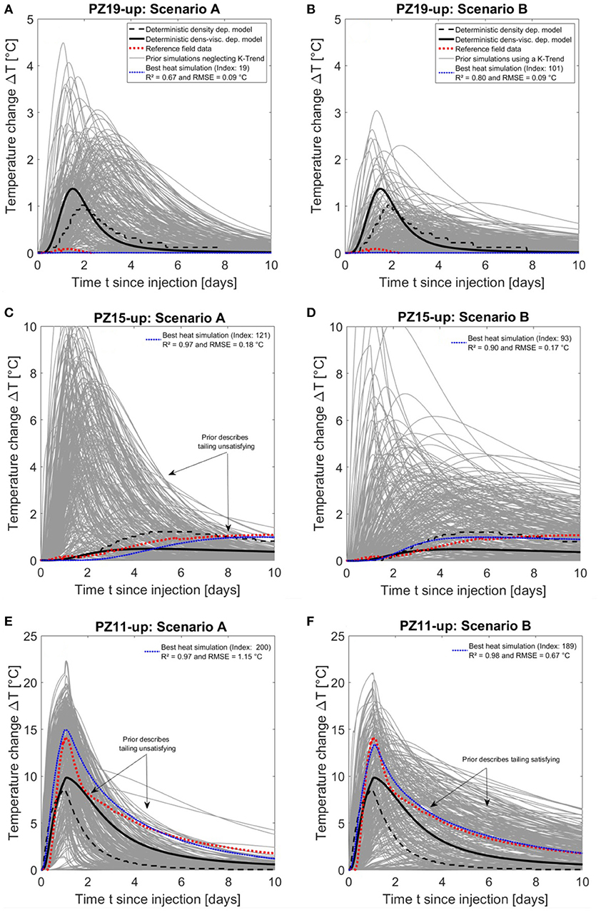
Figure 2. Comparison between deterministic solution, real data and prior + best simulation for both random K-distribution scenarios for Pz19-up (Panel 3): (A) without K-trend (scenario A), (B), with a downwards increasing K-trend (scenario B), for Pz15-up (Panel 2): (C) without K-trend, (D) with K-trend, and for Pz11-up (Panel 1): (E) without K-trend, (F) with K-trend (10 best heat simulations at each observation point are in Supplementary File). The index of the best solution refers its number within the 250 simulations.
The change of the dynamic viscosity, e.g., at the peak-time for Pz11-up about 25 % (upper screen), has a significant effect on the simulated temperature, while the effect of density is limited (0.02 %) (Figures 2E,F, 3). Accounting for this effect allows slight improvement to the fit with the observed heat breakthrough curve at Pz11-up and Pz15-up using a deterministic approach (Figures 2C–F). The simulated peak, e.g., at Pz11-up is slightly improved, as well as the tailing, but the overall fit is still not satisfying for all three observation points.
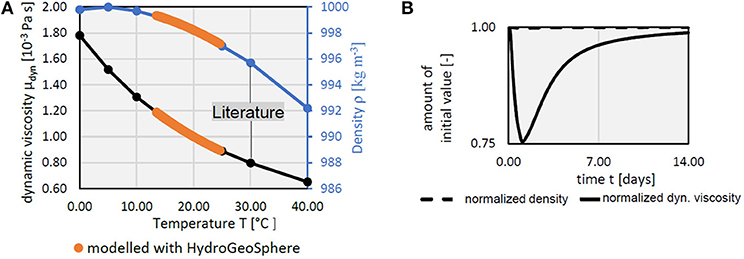
Figure 3. Variation of density and water viscosity influenced by the injected heat observed at PZ11-up as absolute change (A) and relative change (B). (Hoffmann et al., 2018).
Monte-Carlo realizations surround the real data set of the heat tracer at all three points (Figure 2). It highlights the influence of spatial parameter heterogeneity on the resulting breakthrough curves. However, the prior of scenario A seems to be falsified by the tailing part of the curve observed in Pz11-up and Pz15-up (Figures 2C,E). Clearly, scenario B considering the observed vertical downwards increasing K-trend, and describes the tailing part of the curve more realistically compared to the deterministic approach and scenario A (e.g., compare Figures 2E,F). For Pz15-up and Pz19-up the best simulation allows representing the reference data more accurately, compared to the deterministic solutions (Figures 2A–D). Again, scenario B gives more realistic solutions than ignoring any trend in the simulations.
Selecting the 10 best heat simulations from both prior scenarios for all observation points at panels 1 to 3, upper and lower screen, further confirms that considering a vertical downwards increasing K-trend in the simulations is a more realistic description of spatial heterogeneity (referring to “Supplementary Material Figures 1–4”). At panel 3 the observed data fluctuates around a temperature change of 0 °C, without a significant peak. Thus, the solution simulation with ΔT = 0 °C is identified as the best one. The modeled ΔT = 0 °C is exactly zero for the simulation because it corresponds to a set of parameters where diffusion is larger than advection transport; the heat therefore does not reach panel 3. These results stress the need for a more realistic prior-uncertainty quantification and falsification of prior hypotheses. Here, a purely random K-field can be considerably improved by including sedimentological observations that the advocated procedure is capable of taking advantage of it.
Previous paragraphs do not integrate the joint heat and solute breakthrough curves at the pumping well (located 5 m downstream from panel 3). Here, the deterministic model solution calibrated on heat data only (Klepikova et al., 2016), including now both the density and viscosity changes, fails to predict the heat and solute tracers behaviors at the pumping well (Figures 4A,B. Note that the solution depending on density only is not realistic and is not shown).
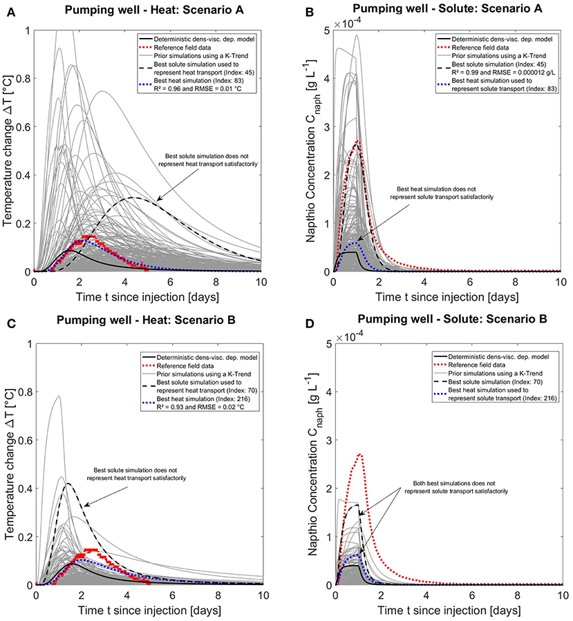
Figure 4. Heat and solute simulation results at the pumping well ignoring any trend (A,B) and considering a downwards increasing K-trend (C,D) compared with the deterministic density-viscosity model. Best heat and solute simulation were used to visualize the complementary tracer (Note that the simulations which consider only the density dependence to temperature and not the viscosity dependence are not shown and rejected as they are not realistic enough).
Monte-Carlo simulations, with the random K-field without trend (scenario A), surround heat and solute observed data (Figures 4A,B), adding indications that spatial heterogeneity is necessary to generate realistic predictions. The best simulation for the observed heat signal using equation (2) (R2 = 0.96, RMSE = 0.01 °C) is however different than the one for the solute signal (R2 = 0.99, RMSE = 1.2·10−5 g L−1). Thus, the best heat simulation poorly predicts the solute signal and vice versa (Figures 4A,B). For the random K-field with the vertical downwards increasing K-trend (scenario B), the heat breakthrough at the pumping well is not as well simulated as in the intermediate panels and the solute breakthrough concentrations are strongly underestimated, even though the time occurrence of the peak seems to be correctly predicted (Figures 4C,D). Near the pumping well, the tracer is intensively diluted due to the high pumping rate (30 m3h−1), making the heterogeneity around this well crucial for explaining the breakthrough curve (see in Discussion section).
The K-fields corresponding to the best heat and solute simulations describing the tracer breakthrough curves at the pumping well using scenario A are largely heterogeneous (Figures 5A,B). However, for both tracers, K-distributions are slightly different, which explains in parallel to the less good modeling of the tailing (Figure 2), why scenario A is not suitable to adequately describe complementary tracer movement (Figures 4, 5). The injected heat forms a plume around the injection well enlarging with time by conduction and advection, while its temperature amplitude decreases (Figure 5C). Further, the solute prefers mainly the high hydraulic conductivity pathways, faster in the lower part than in the upper part (Figure 5D). Both tracers are best described by two different parameter distributions and only stochastic inversion could here result in simulations fitting both, while deterministic inversion finding one global parameterization, may tend to derive a smoothed parameter distribution poorly fitting the data. However, it should be stressed that this prior (scenario A) would not be able to reproduce the observations in intermediate panels. For the K-field and tracer distribution of scenario B (Supplementary Material Figure 5), the best solute tracer simulation displays a strongly heterogeneous model with preferential flow paths, while for heat, a more homogenous K-field respecting the observed trend in the borehole drillings sedimentology (Figure 1B) is found.
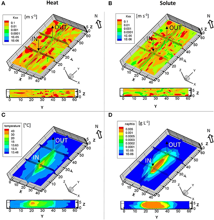
Figure 5. Simulated results at the pumping well using a prior with no K-trend distribution (Scenario A): Spatial K-distribution as obtained for the picked up best simulation for (A) heat data and (B) for the best napthionate simulation. Corresponding simulated tracer plumes for best simulation for (C) heat data and (D) for napthionate data. Under each 3D visualization, a vertical 2D profile is shown along the gradient axis from the injection well through panels 1, 2, and 3, and down to the pumping well.
These single local best realizations, for each observation point, do not explain the full data set, further highlighting the role of local heterogeneity on the measured signals. This probably explains why the global fit of the deterministic solution is poor and highlights the need for more realistic priors instead of trying to find unique parameterization describing reality.
For the Hermalle-sous-Argenteau test site, the prior considering a vertical downwards increasing K-trend seems to better represent the overall hydraulic conditions (until panel 3) and constitutes a better prior assumption than neglecting any K-trend. However, it seems to be somewhat falsified between the last panel and the pumping well in terms of solute concentration amplitude. This suggests that the current parameterization still oversimplifies the heterogeneity of the deposits at a larger scale and cannot be used for inversion or prediction. New hypotheses should be formulated, or new data collected to identify the specific processes taking place between the third panel and the pumping well. Existing ERT transects (Hermans et al., 2015a,b) and newly acquired cross-hole GPR sections are promising tools to image heterogeneity patterns with a higher resolution and at a larger scale.
Distance Based Sensitivity Analysis
The 250 generated models from scenario B are further used for the distance-based global sensitivity analysis. The distance metrics (Equation 2) between pairs of Monte-Carlo simulations is calculated and used as starting point for DGSA. The sensitivity analysis investigates the global simulation parameter values within their given range (Table 1) and the spatial heterogeneity. To analyze spatial heterogeneity, the K-fields from Monte-Carlo simulations are represented using orthogonal basis vectors computed through principal component analysis (PCA) with 250 observation rows and 140,140 corresponding cell K-values as columns (in total: 35,035,000 K values). Only the first 15 principal components are retained and used as an approximate measure of heterogeneity. While, those 15 first dimensions explain only 23 % of the total variance in K, the first three principal components together describe 9.6 % of the variance. The small amount of explained variance is related to the strongly variating K-values from one simulation to the other. The 15 corresponding PCA scores are further included in the sensitivity analysis to characterize the role of spatial heterogeneity.
The sensitivity analysis results for the heat signal at the panels 1, 2, and 3 in relation are presented in Figures 6A,C,E. Figures 6B,D,F show the corresponding classification of the 250 models in three clusters. Clusters are used to group the simulations according to their response (i.e., the first cluster contains simulations with high temperature far above the reference data, the second contains simulations with temperature below the reference data and the third group consists in simulations around the reference data). Using three clusters gives satisfactory results in this case.
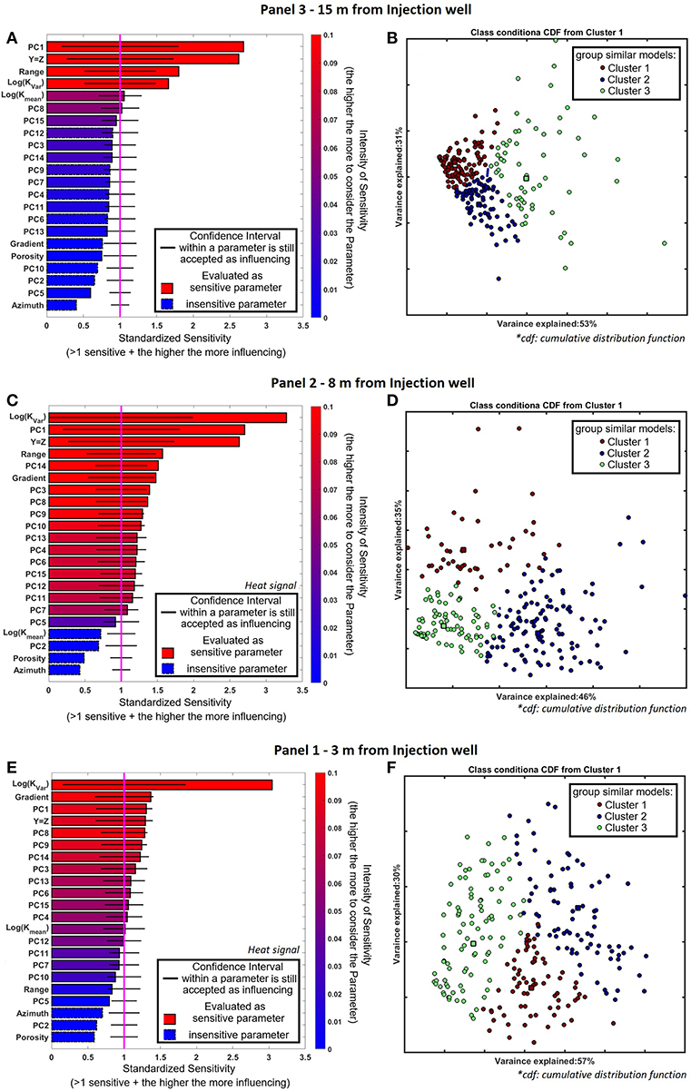
Figure 6. Distance-based sensitivity analysis using the scenario B heat signals at (A) Panel 3, (C) Panel 2, (E) Panel 1, related to the corresponding cluster cumulative distribution function (CDF) for (B) Panel 3, (D) Panel 2, and (F) Panel 1. The square within each cluster in (B), (D), and (F) is the center of mass of each cluster.
The sensitivity of a parameter is computed based on the difference between its cumulative distribution function (cdf) in each of the cluster compared to the global cdf. Significant differences mean that the parameter is considered as sensitive. For all panels, the resampling quantile of the distance is α = 0.95 (we refer to Park et al. (2016) for the detailed explanations of parameters used in DGSA).
The global “log(Kvar)” is the most sensitive parameter at Panel 1 and 2 (Figures 6C,E). Its sensitivity decreases within the third panel (Figure 6A) while “log(Kmean)” is getting more sensitive (Figures 6A,C,E). The influence of the first component of spatial heterogeneity “PC1” is large at every distance from the injection well. The increasing sensitivity and influence of “PC1” with distance from the injection well is related to the hydraulic conductivity in the direction of the gradient, which indicates a strong link to preferential pathways (Figures 6A,C,E). For the first two panels, most PCA components are sensitive. This is in accordance with the previous results, showing that the introduced K-trend is crucial to explain the observed breakthrough curves (section Prior uncertainty investigation). The global parameter “gradient” shows a decreasing sensitivity with distance. The sensitivity of the gradient highlights the influence of uncertain boundary conditions on the simulations. The fluxes around the injection well are crucial to initiate the tracer transport (Figures 6A,C,E). The global “porosity” and the “azimuth” are, at all three panels, a much less sensitive parameter for the strong advective system at Hermalle-sous-Argenteau. The variance explained in the low dimensional space is relatively constant over all three panels, but the clusters are getting closer to each other (Figures 6B,D,F). The sensitivity analysis further indicates that the scale of heterogeneity playing a role on the tracer distribution at panel three is different. The vertical K-trend is not sufficient anymore to explain the observations. It underpins that more realistic imaged preferential pathways (e.g., using improved imaging methods like full-waveform GPR inversion) are probably necessary to understand the heterogeneity surrounding the pumping well.
The sensitivity analysis results at the pumping well using the heat and solute signals using the 250 simulation of scenario B are presented in Figure 7. For the heat and the solute signals, the “log(Kmean)” is more sensitive than the “log(Kvar)” and the “PC1,” “PC2,” and “PC3.” The local heterogeneity is still sensitive and important to consider, but the results are less sensitive to small scale heterogeneity as mostly “PC1” to “PC4” are sensitive. For solute transport, “porosity” is also a sensitive parameter to be considered (Figures 7A,B), probably due to its direct effect on advection velocity. The analysis supports that simulating complementary tracer behavior requires a realistic description of heterogeneity.
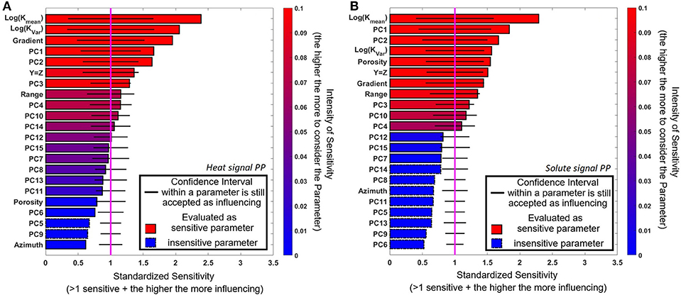
Figure 7. Sensitivity analysis at the pumping well using the scenario B for (A) heat and (B) solute signals.
The sensitivity analysis of the pumping well simulations using scenario B is extended by using alternatively the synthetic velocity ratio vheat/vsol as prior response for the DGSA (Figure 8). Replacing the breakthrough curve as model response by the velocity ratio vheat/vsol, averages the model response over the complete transport path.
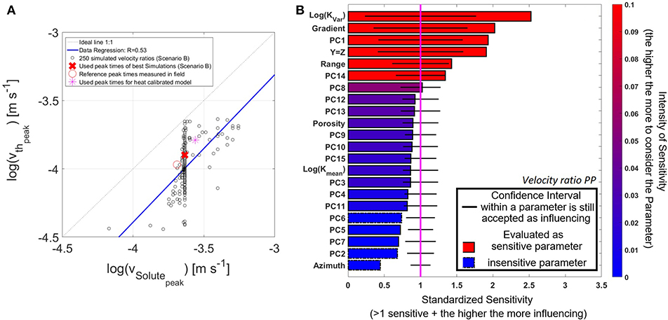
Figure 8. (A) Velocity ratio vheat/vsol comparison using the peak times of the heat and solute breakthroughs generated with Monte-Carlo using Scenario B (K-Trend). (B) Sensitivity results using the derived velocity ratio vheat/vsol as prior responses for DGSA.
As a reference, the field measured derived modal velocities at the peak time of heat (i.e., Rth = 1 ≥ wavefront velocity) and solute at the pumping well are:
Using the assumption of Rth = 1, for scenario B (Figure 8A), the obtained velocity ratios are less spread around the observed data. Many solute velocities forecasts have the same value, but with a different corresponding heat velocity (Figure 8A). This is an indication that the heat signal provides more information, while the variance of the solute velocity responses decreases.
Applying now the DGSA using this alternative prior response, the sensitivity of “porosity” is now less strong than in the solute case, but stronger than in the heat case (Figures 7, 8B). Then, similar to panel 1 to 3, the “log(KVar),” “gradient,” and “PC1” are the most sensitive parameter at the pumping well (Figure 8B). Interestingly, the velocity ratio seems to be not directly sensitive to “log(Kmean),” but on the global heterogeneity (Kvar and range), spatial heterogeneity (PC1) and fluxes (gradient). This is a clear indication that preferential flow paths, being the result of an interaction between K-heterogeneity and gradient, is the main reason for the variation in velocity ratio.
At this stage, it can be assessed that the joint heat-solute tracer experiment results are indeed better represented by a K-distribution with a vertical downwards increasing K-trend. The prior with the K-trend is the current best heterogeneity representation for Hermalle-sous-Argenteau test site between the injection well and panel 3. However, this K-trend is not representative for the part of the simulated domain between the third panel and the pumping well as shown by the Monte-Carlo prior investigation and the DGSA results. This highlights how important a not-falsified prior is for robust decision making, and that every model containing approximations must be use with care for predictions. Furthermore, if the proposed prior seems valid at the local scale, it is not sufficient to explain all observations made at the site. The latter probably requires the inclusion of another level of heterogeneity, accounting for the change of behavior for the tracer.
Discussion
In the field tracer experiment, the heat tracer arrives 1 day after the solute transport and the recovered energy at the pumping well is very low. This delay is a consequence of the different transport processes, mainly the retardation effect related to heat conduction in the solid phase and in the immobile water. For example, the heat tracer test provides useful information to better understand the matrix processes quantifying the immobile water part. This complementary behavior helps to better characterize the actual transport processes occurring in the aquifer, in particular the preferential flow paths.
The previous existing calibrated model was based on heat tracing data only. The new numerical model implemented in the framework of the presented study, showed that the dynamic viscosity has a strong impact on simulated temperature values even in a narrow temperature range. It clearly appeared that this model was failing to reproduce the observed solute concentrations at the pumping well. All attempts to find one single deterministic model fitting both tracer data failed, illustrating the difficulty to approximate solute advection and heat conduction/storage with one single (smoothed) spatial parameter distribution. Even if a global minimum was found, any prediction would remain based on a simplified model with limited prediction capabilities.
To overcome limitations of the deterministic approach, and to avoid full stochastic inversions, performing prior parameter uncertainty investigation using multiple Monte-Carlo realizations offers the possibility to generate more geologically realistic subsurface parameter distributions. Compared to transdimensional inference, which although stochastic in essence and would involve some degree of simplification or parsimony (Sambridge et al., 2012), keeping the full variability in the model is necessary to generate realistic predictions. Thus, in this study, the analysis of those simulations revealed that increasing the spatial heterogeneity of the alluvial deposits allows to better reproduce the observed breakthrough curves. The considered prior uncertainty generates a range of possible outcomes surrounding the observed data. The specific behavior of the breakthrough curves, such as the sharp decrease of temperature after the peaks, is much better reproduced. It is also clearly shown that approximations made in deterministic approaches (e.g., using smoothed K-distributions), strongly influence the results and contribute to higher uncertainty. Furthermore, it appeared that modeling the deposits with two separate layers did not allow the reproduction of the tailing part of the breakthrough curves, whereas a continuous distribution with a vertical downwards increasing trend was more able to model this behavior. However, it was also shown that the used vertical K-trend seems not to be appropriate, i.e., between the third panel and the pumping well. Investigating prior uncertainty here has greatly helped to update the previous conceptual ideas that were mostly based on simple investigations like borehole log description.
The proposed prior with the K-trend is consistent with all observation points (Panel 1 to 3) except the pumping well and Pz18, 19 in the lower aquifer part. Between panel 3 and the pumping well, there are likely preferential flow paths influencing the tracer behaviors, not properly described by the proposed prior. The latter was mainly built based on the high borehole density from intermediate panels. In the original log description of the pumping well (drilled in the 90's), there is no grain size trend described. One possibility is therefore that the strongly heterogeneous alluvial deposits cannot be described by a single simplified parameterization (here Gaussian simulations with a trend) but must include more heterogeneity at the larger scale (for example different vertical trend). It appears that lateral variations occur in the aquifer, stressing the need for a more global description of the heterogeneity, including larger scale sedimentological structures such as channels, and advanced integration of secondary data such as geophysical tomographies (e.g., Hermans et al., 2015a). Indeed, geophysical data acquired on the site showed lateral variations in electrical resistivity related to gravel structures (Hermans and Irving, 2017). A trade-off between the acquisition of new data to refine understanding and cost-affordable field studies must be found. In this framework, the combination of hydrogeological testing (such as joint-heat tracer tests) with static and time-lapse geophysical data (such as GPR and ERT) at an early stage of site characterization is the key to acquire informative data sets at limited costs.
The prior uncertainty analysis also reveals that each specific temperature breakthrough observation is better reproduced by a different prior realization and, therefore, spatial parameter distribution. This clearly identifies spatial heterogeneity as having a major influence on the simulation results. The solute tracer breakthrough at the pumping well is better represented with models showing preferential flow paths, largely influencing advective-dispersive processes. In contrast, temperature observations in the intermediate panels and at the pumping well seem to be better represented with a slightly more homogeneous model, as conduction is indeed important. This might indicate that a significant part of the pore space is occupied by immobile water. This interpretation shows clearly that the previous conceptual model represented by Peclet numbers of 300 (in the upper layer) and 14,000 (in the lower layer) is not adequate. Furthermore, it shows that the use of a heat tracer alone is not necessarily a good choice to calibrate a model, especially if solute transport should be predicted. Trying to use one single deterministic model parametrization is limited here by two points: (1) complementary tracers cannot really predict each other with classic underlying simplifying assumptions and one parametrization and (2) heterogeneity patterns are complex, meaning that highly parameterized inversion might fail to converge toward a realistic solution.
Similarly, stochastic inversion or optimization techniques might be very complicated to tune to convergence in such a complex layout. Here starts the potential of advanced prediction approaches such as Bayesian Evidential Learning. An informative prior sampled by multiple realizations containing complementary tracer processes might be directly used for prediction if a statistical relationship can be found between data and prediction variables. This kind of approach is probably very promising for the future of hydrogeological modeling where the full, explicit inversion fails due to the lack of sufficient qualitative data to constrain the geometry of the deposits. Some uncertainty component might be irreducible and impossible to resolve through inversion methodologies. Approaches such as BEL, combined with an in-depth prior uncertainty analysis, can therefore be a good way to account for those in prediction uncertainty assessment in a computational efficient way.
The fact that a global sensitivity analysis shows different sensitivity patterns for heat and solute responses, here the porosity, is another indication of the complementarity between the tracers. If heterogeneity is more realistically represented by the K-Trend distribution (scenario B), heat seems, in comparison to solute, insensitive to porosity. Although, the Hermalle-sous-Argenteau site is characterized by a strongly advective system, the heat data set remains dominated by the effect of conduction. Heat is mainly stored around the injection well and is only slightly and very slowly withdrawn from the reservoir at the pumping well. Some parts of the heat are transported fully through conduction (immobile water and solid matrix).
The presented study also shows that using the Euclidean distance for the distance-based global sensitivity analysis, might be of limited interest for data sets containing strong complementary behavior. It can result in different sensitivities between needed parameterization for the related output. An alternative proposition is to use the velocity ratio as a proxy for the model response, as it allowed to clearly identify preferential flow paths as the main explanation for the difference in tracer behaviors.
Conclusion
New innovative imaging methods, namely joint heat and solute tracer tests were combined with advanced field data analysis tools to better assess preferential pathways and associated uncertainty in complex alluvial deposits. This paper demonstrates the limitation of deterministic inversion approaches in capturing the complementary behavior of heat and solute tracers. To overcome those limitations, a prior-uncertainty investigation and a heat-solute velocity comparison are applied. Monte-Carlo simulations are used to investigate the range of simulated data and are complemented by a distance-based global sensitivity analysis. The main results are:
1) Heat injection with absolute measured temperature signals between 10 and around 40 °C, as observed for common heat tracer tests, requires considering dynamic viscosity effects in the simulations.
2) Although much effort has been done to calibrate a deterministic model on the complex heat tracer data, the underlying approximations always yield a too smooth K distribution, failing to predict the solute breakthrough curve.
3) In comparison to (over) simplified deterministic models, stochastic models allow for the relaxation of those approximations, and also consider K-fields in conjunction with heterogeneity. Thus, stochastic models using Monte-Carlo reproduce measurements significantly better. They can better reproduce specific behaviors of breakthrough curves (e.g., the tailing). A simple falsification procedure allows to easily reject prior hypotheses inconsistent with the data. It reveals that a single parameterization is not sufficient to fully describe the complex behavior observed at Hermalle-sous-Argenteau. Due to complex spatial heterogeneity and different behavior of the tracers, the simultaneous fitting of all observation points seems to be almost impossible using explicit inversion approaches. Approaches focusing on the prediction and avoiding model inversion (e.g., such as BEL) might be more successful.
4) The global sensitivity analysis reveals that heat seems to be less sensitive to advection parameters like porosity than solute, as was expected based on previous studies. For the strong advective system at Hermalle-sous-Argenteau, heat transport does not seem to be affected by porosity, as long as realistic heterogeneity is considered, using a vertical downwards increasing K-Trend distribution respecting the borehole sedimentology. Indicators linked to local spatial heterogeneity are sensitive parameters for both heat and solute transport, stressing the need to use an adequate prior description of the deposits, a prerequisite for any stochastic Bayesian inversion.
5) The tracer velocity comparison shows that the prior and the sampled Monte-Carlo simulations yield a better representation of the joint heat and solute behavior as observed on the field. This is a key point for further research steps in modeling and predicting the transport processes in this aquifer.
Data Availability
Note that the datasets analyzed for this study must be stored on the H+ Network (http://hplus.ore.fr/en/enigma/data-hermalle) as a mandatory part of the funding project (ENIGMA ITN). The files are ready and currently under upload. We guarantee, that they will be uploaded as it is a mandatory requirement. Codes for DGSA are freely available at https://github.com/SCRFpublic.
Author Contributions
RH generated the results, did most of the writing and the layout of the contribution. TH was the main supervisor and motivator for the paper, contributed mostly to the redaction and writing part as well as assisted actively the modeling part. AD ensured the financial support of the joined tracer tests in Hermalle, did the supervision of the previous works (Wildemeersch et al., 2014; Klepikova et al., 2016), contributed in conceptual and methodological discussions, helped for the writing part and is the main promoter of the Ph.D. of RH. PG reviewed the paper from a global and external position and is the second promoter of the Ph.D. project of RH.
Conflict of Interest Statement
The authors declare that the research was conducted in the absence of any commercial or financial relationships that could be construed as a potential conflict of interest.
Acknowledgments
This work is part of the Ph.D.-thesis of RH in the ENIGMA ITN framework. ENIGMA has received funding from European Union's Horizon 2020 research and innovation programme under the Marie Sklodowska-Curie Grant Agreement N°722028. We thank Jef Caers for our fruitful discussion about the results of the sensitivity analysis. Further, we are thankful for the review and the fruitful exchange with three reviewers and the associated Editor.
Supplementary Material
The Supplementary Material for this article can be found online at: https://www.frontiersin.org/articles/10.3389/feart.2019.00108/full#supplementary-material
References
Alcolea, A., Carrera, J., and Medina, A. (2006). Pilot points method incorporating prior information for solving the groundwater flow inverse problem. Adv. Water Resources 29, 1678–1689. doi: 10.1016/j.advwatres.2005.12.009
Anderson, M. P. (2005). Heat as a ground water tracer. Ground Water 43, 951–968. doi: 10.1111/j.1745-6584.2005.00052.x
Brunner, P., and Simmons, C. T. (2012). HydroGeoSphere: a fully integrated, physically based hydrological model. Ground Water 50, 170–176. doi: 10.1111/j.1745-6584.2011.00882.x
Caers, J. (2011). Modeling Uncertainty in Earth Sciences. Wichester: Wiley-Blackwell. doi: 10.1002/9781119995920
Davis, S. N., Thompson, G. M., Bentley, H. W., and Stiles, G. (1980). Ground-water tracers—a short review. Ground Water 18, 14–23. doi: 10.1111/j.1745-6584.1980.tb03366.x
Doherty, J. (1994). “PEST: a unique computer program for model-independent parameter,” in Water Down Under, Vol. 94. 551–554. Retrieved from https://search.informit.com.au/documentSummary;dn=752715546665009;res=IELENG (accessed May 10, 2019).
Doherty, J. (2003). Ground water model calibration using pilot points and regularization. Ground Water 41, 170–177. doi: 10.1111/j.1745-6584.2003.tb02580.x
Fenwick, D., Scheidt, C., and Caers, J. (2014). Quantifying asymmetric parameter interactions in sensitivity analysis: application to reservoir modeling. Math Geosci. 46, 493–511. doi: 10.1007/s11004-014-9530-5
Ferré, T. P. A. (2017). Revisiting the relationship between data, models, and decision-making. Groundwater 55, 604–614. doi: 10.1111/gwat.12574
Fuchs, J. W., Fox, G. A., Storm, D. E., Penn, C. J., and Brown, G. O. (2009). Subsurface transport of phosphorus in riparian floodplains: influence of preferential flow paths. J. Environ. Q. 38, 473–484. doi: 10.2134/jeq2008.0201
Heeren, D. M., Miller, R. B., Fox, G. A., Storm, D. E., Halihan, T., and Penn, C. J. (2010). Preferential flow effects on subsurface contaminant transport in alluvial floodplains. Trans. ASABE 53, 127–136. doi: 10.13031/2013.29511
Hermans, T. (2017). Prediction-focused approaches: an opportunity for hydrology. Groundwater 55, 683–687. doi: 10.1111/gwat.12548
Hermans, T., and Irving, J. (2017). Facies discrimination with electrical resistivity tomography using a probabilistic methodology: effect of sensitivity and regularisation. Near Surface Geophys. 15, 13–25. doi: 10.3997/1873-0604.2016047
Hermans, T., Nguyen, F., and Caers, J. (2015a). Uncertainty in training image-based inversion of hydraulic head data constrained to ERT data: workflow and case study. Water Resources Res. 51, 5332–5352. doi: 10.1002/2014WR016460
Hermans, T., Nguyen, F., Klepikova, M., Dassargues, A., and Caers, J. (2018). Uncertainty quantification of medium-term heat storage from short-term geophysical experiments using bayesian evidential learning. Water Resources Res. 54, 2931–2948. doi: 10.1002/2017WR022135
Hermans, T., Oware, E., and Caers, J. (2016). Direct prediction of spatially and temporally varying physical properties from time-lapse electrical resistance data: direct forecast from tl resistance data. Water Resources Res. 52, 7262–7283. doi: 10.1002/2016WR019126
Hermans, T., Wildemeersch, S., Jamin, P., Orban, P., Brouyère, S., Dassargues, A., et al. (2015b). Quantitative temperature monitoring of a heat tracing experiment using cross-borehole ERT. Geothermics 53, 14–26. doi: 10.1016/j.geothermics.2014.03.013
Hoffmann, R., Hermans, T., Goderniaux, P., and Dassargues, A. (2018). “Prior uncertainty investigation of density-viscosity dependent joint transport of heat and solute in alluvial sediments,” in Computational Methods in Water Resources XXII - Bridging Gaps Between Data, Models, and Predictions (Saint Malo). Retrieved from: https://www.irisa.fr/sage/jocelyne/CMWR2018/pdf/CMWR2018_paper_166.pdf (Abstract No. 166).
Irvine, D. J., Simmons, C. T., Werner, A. D., and Graf, T. (2015). Heat and solute tracers: how do they compare in heterogeneous aquifers? Groundwater 53, 10–20. doi: 10.1111/gwat.12146
Klepikova, M., Wildemeersch, S., Hermans, T., Jamin, P., Orban, P., Nguyen, F., et al. (2016). Heat tracer test in an alluvial aquifer: field experiment and inverse modelling. J. Hydrol. 540, 812–823. doi: 10.1016/j.jhydrol.2016.06.066
Krzanowski, W. J. (2000). Principles of Multivariate Analysis: A User's Perspective, Revised Edn. New York, NY: Oxford University Press.
Ma, R., and Zheng, C. (2009). Effects of density and viscosity in modeling heat as a groundwater tracer. Ground Water 48, 380–389. doi: 10.1111/j.1745-6584.2009.00660.x
Maliva, R. G. (2016). Aquifer Characterization Techniques. Cham: Springer International Publishing. doi: 10.1007/978-3-319-32137-0
Oware, E. K., Moysey, S. M. J., and Khan, T. (2013). Physically based regularization of hydrogeophysical inverse problems for improved imaging of process-driven systems. Water Resources Res. 49, 6238–6247. doi: 10.1002/wrcr.20462
Park, J., and Caers, J. (2018). “Sensitivity analysis of reservoir forecasts with both global and local model variables,” in SCERF Annual Meeting (Stanford, CA).
Park, J., Yang, G., Satija, A., Scheidt, C., and Caers, J. (2016). DGSA: a matlab toolbox for distance-based generalized sensitivity analysis of geoscientific computer experiments. Comput. Geosci. 97 (Suppl. C), 15–29. doi: 10.1016/j.cageo.2016.08.021
Ptak, T., Piepenbrink, M., and Martac, E. (2004). Tracer tests for the investigation of heterogeneous porous media and stochastic modelling of flow and transport—a review of some recent developments. J. Hydrol. 294, 122–163. doi: 10.1016/j.jhydrol.2004.01.020
Remonti, M., and Mori, P. (2016). The stochastic approach in groundwater modeling for the optimization of hydraulic barriers: the stochastic approach in groundwater modeling for the optimization of hydraulic barriers. Remediat. J. 26, 109–120. doi: 10.1002/rem.21462
Renard, P. (2007). Stochastic hydrogeology: what professionals really need? Ground Water 45, 531–541. doi: 10.1111/j.1745-6584.2007.00340.x
Rojas, R., Feyen, L., and Dassargues, A. (2009). Sensitivity analysis of prior model probabilities and the value of prior knowledge in the assessment of conceptual model uncertainty in groundwater modelling. Hydrol. Process. 23, 1131–1146. doi: 10.1002/hyp.7231
Sambridge, M., Bodin, T., Gallagher, K., and Tkalcic, H. (2012). Transdimensional inference in the geosciences. Philos. Trans. R. Soc. A 371:20110547. doi: 10.1098/rsta.2011.0547
Sarris, T. S., Close, M., and Abraham, P. (2018). Using solute and heat tracers for aquifer characterization in a strongly heterogeneous alluvial aquifer. J. Hydrol. 558, 55–71. doi: 10.1016/j.jhydrol.2018.01.032
Scheidt, C., Li, L., and Caers, J. (2018). Quantifying Uncertainty in Subsurface Systems. Hoboken, NJ; Washington DC: John Wiley and Sons & American Geophysical Union. doi: 10.1002/9781119325888
Therrien, R., McLaren, R. G., Sudicky, E. A., and Panday, S. M. (2010). HydroGeoSphere: a Three-Dimensional Numerical Model Describing Fully-Integrated Subsurface and Surface Flow and Solute Transport. Waterloo, ON: Groundwater Simulations Group, University of Waterloo.
Wildemeersch, S., Jamin, P., Orban, P., Hermans, T., Klepikova, M., Nguyen, F., et al. (2014). Coupling heat and chemical tracer experiments for estimating heat transfer parameters in shallow alluvial aquifers. J. Contam. Hydrol. 169, 90–99. doi: 10.1016/j.jconhyd.2014.08.001
Keywords: joint heat and solute tracer tests, density-viscosity dependent flow and transport, alluvial sediments, preferential flow paths, uncertainty investigation, distance-based global sensitivity analysis, principal component analysis
Citation: Hoffmann R, Dassargues A, Goderniaux P and Hermans T (2019) Heterogeneity and Prior Uncertainty Investigation Using a Joint Heat and Solute Tracer Experiment in Alluvial Sediments. Front. Earth Sci. 7:108. doi: 10.3389/feart.2019.00108
Received: 30 November 2018; Accepted: 26 April 2019;
Published: 29 May 2019.
Edited by:
Frederick Delay, Université de Strasbourg, FranceReviewed by:
Jean-Francois Girard, UMR7516 Institut de Physique du Globe de Strasbourg (IPGS), FranceBruno Cheviron, National Research Institute of Science and Technology for Environment and Agriculture (IRSTEA), France
Copyright © 2019 Hoffmann, Dassargues, Goderniaux and Hermans. This is an open-access article distributed under the terms of the Creative Commons Attribution License (CC BY). The use, distribution or reproduction in other forums is permitted, provided the original author(s) and the copyright owner(s) are credited and that the original publication in this journal is cited, in accordance with accepted academic practice. No use, distribution or reproduction is permitted which does not comply with these terms.
*Correspondence: Richard Hoffmann, cmljaGFyZC5ob2ZmbWFubkB1bGllZ2UuYmU=