Abstract
With the advent of the two Sentinel-1 (S1) satellites, Synthetic Aperture Radar (SAR) data with high temporal and spatial resolution are freely available. This provides a promising framework to facilitate detailed investigations of surface instabilities and movements on large scales with high temporal resolution, but also poses substantial processing challenges because of storage and computation requirements. Methods are needed to efficiently detect short term changes in dynamic environments. Approaches considering pair-wise processing of a series of consecutive scenes to retain maximum temporal resolution in conjunction with time series analyses are required. Here we present OSARIS, the “Open Source SAR Investigation System,” as a framework to process large stacks of S1 data on high-performance computing clusters. Based on Generic Mapping Tools SAR, shell scripts, and the workload manager Slurm, OSARIS provides an open and modular framework combining parallelization of high-performance C programs, flexible processing schemes, convenient configuration, and generation of geocoded stacks of analysis-ready base data, including amplitude, phase, coherence, and unwrapped interferograms. Time series analyses can be conducted by applying automated modules to the data stacks. The capabilities of OSARIS are demonstrated in a case study from the northwestern Tien Shan, Central Asia. After merging of slices, a total of 80 scene pairs were processed from 174 total input scenes. The coherence time series exhibits pronounced seasonal variability, with relatively high coherence values prevailing during the summer months in the nival zone. As an example of a time series analysis module, we present OSARIS' “Unstable Coherence Metric” which identifies pixels affected by significant drops from high to low coherence values. Measurements of motion provided by LOSD measurements require careful evaluation because interferometric phase unwrapping is prone to errors. Here, OSARIS provides a series of modules to detect and mask unwrapping errors, correct for atmospheric disturbances, and remove large-scale trends. Wall clock processing time for the case study (area ~9,000 km2) was ~12 h 4 min on a machine with 400 cores and 2 TB RAM. In total, ~12 d 10 h 44 min (~96%) were saved through parallelization. A comparison of selected OSARIS datasets to results from two state-of-the-art SAR processing suites, ISCE and SNAP, shows that OSARIS provides products of competitive quality despite its high level of automatization. OSARIS thus facilitates efficient S1-based region-wide investigations of surface movement events over multiple years.
1. Introduction
Surface movement events are abundant in high-mountain environments and further activation is anticipated under sustained climate change, e.g., through thawing permafrost on slopes or unstable moraines in deglaciated settings (Heckmann et al., 2016). To date, analyses of the timing, location, and magnitude of such events are limited to few sites where detailed monitoring programs have been established. Synthetic Aperture Radar (SAR) interferometry (InSAR) has proven its large potential to detect and analyze surface movements (e.g., Gabriel et al., 1989; Massonnet and Feigl, 1998); however, until recently such investigations were typically limited to individual events and regions favorable for obtaining high coherence pairs owing to long temporal baselines and low spatial resolution. This situation changed in recent years and particularly with the advent of the European Space Agency's two Copernicus Sentinel-1 satellites (S1; e.g., Malenovsky et al., 2012; Torres et al., 2012) providing freely available, high-quality C-band SAR data with high temporal and spatial resolution (Rucci et al., 2012; Jung et al., 2013; Yagüe-Martínez et al., 2016). S1 data thus provide a promising framework to facilitate broad applications of detailed SAR- and interferometry-based surface changes as demonstrated by a rapidly increasing portfolio of studies from all classic domains of InSAR applications, including surface deformation through earthquakes (e.g., Grandin et al., 2016; Polcari et al., 2016), thawing permafrost (e.g., Strozzi et al., 2018), or volcanoes (e.g., González et al., 2015), surface movements by landslides (e.g., Bejar et al., 2017; Kalia, 2018), glacier ice velocities (e.g., Sánchez-Gámez and Navarro, 2017), and damage assessment (e.g., Plank, 2014; Olen and Bookhagen, 2018). Furthermore, the short revisit time of 6–12 days opens perspectives toward near real time monitoring applications (e.g., Raspini et al., 2018). Notably, however, the vast majority of S1 InSAR studies still focuses on obtaining maximum precision and detail for individual events and high coherence regions through application of elaborate methods that typically require substantial manual configuration efforts, such as Persistent Scatterer Interferometry (PSI; cf. Ferretti et al., 2001; Crosetto et al., 2016). Conversely, S1's vast potential to investigate comprehensive and detailed time series is hardly being exploited to date.
The new situation poses great challenges to both soft- and hardware, particularly in cases where long time series and thus large stacks of S1 scenes are to be analyzed, often requiring dozens of scenes of several gigabytes each to be processed. A variety of software products specializing in SAR data processing is available today, out of which SNAP (open source, free; cf. ESA, 2018), GMTSAR (open source, free; cf. Sandwell et al., 2011), ISCE (access restricted, free; cf. Rosen et al., 2012), ENVI SARscape (proprietary, commercial; cf. Harris-Geospatial, 2018), GAMMA (binary and source code licenses available, commercial; cf. GAMMA Remote Sensing, 2017), and SARPROZ (binary and source code licenses available, commercial with free demo, cf. SARPROZ, 2018) are the most mature and actively developed products. However, neither of them are designed to efficiently process large stacks of data with a focus on temporal resolution. To our knowledge, to date there is only one tool focusing on generating such comprehensive time series data, the “P-SBAS Processing Chain” (Zinno et al., 2018), which is, however, closed-source and not available to other researchers. Conversely, access to High Performance Computing (HPC) clusters which facilitate parallel processing of large datasets is widespread today.
Here we present OSARIS (Loibl, 2019a), the “Open Source SAR Investigation System” (GNU General Public License), as a framework to process large stacks of S1 data in HPC environments. OSARIS is based on GMTSAR and the “Slurm workload manager” (Yoo et al., 2003). It was designed with a specific focus on applications retaining the full temporal resolution of the input data time series. The GMTSAR package was chosen as the basis because of high processing performance, shell scripting susceptibility, and good potential for parallel implementation. However, configuration of GMTSAR for analysis of comprehensive datasets is challenging. Also, parallel processing schemes are not directly implemented in GMTSAR, leaving much potential for performance optimization. Key development aims of OSARIS were (i) to facilitate simple and efficient configuration for complex S1 processing workflows; (ii) to provide flexible processing schemes for different scenarios, e.g., pair-wise, single master, Small BAseline Subset (SBAS; cf. Berardino et al., 2002); (iii) to parallelize the processing; (iv) to provide a common and efficient structure for output products; (v) to generate analysis-ready data products, and (vi) to foster outputs that can be readily fed into time series and higher level analyses through a common, convenient interface. Consequently, simplification of the configuration workflow and automated adaptation for different processing scenarios was one of the key aims in the development of OSARIS. In this article, we detail the concept and design of the OSARIS framework and demonstrate its capabilities for standard and time series InSAR processing in a case study from the Tien Shan mountain range in Central Asia. The quality of two key processing result datasets, i.e., interferometric phase and coherence, are evaluated in comparison to ISCE and SNAP.
2. Case Study Area and Data
2.1. Study Area
With an extent of ~2,500 km in WNW-ENE direction and an area of ~800,000 km2, the Tien Shan (Chinese for “Celestial Mountains”) is the dominant mountain range in Central Asia. The orogenic belt exhibits a pronounced basin and range structure with the highest peak at 7,439 m a.s.l. (Kyrgyz, Jengish Chokusu; Russian, Pik Pobedy) and the lowest point at 154 m b.s.l. in the Turfan depression. As a consequence of active tectonics and rugged topography, the Tien Shan is a highly dynamic region exhibiting a variety of surface movement processes well-suited to InSAR studies, including measurements of tectonically induced ground deformation (e.g., Goode et al., 2011; Neelmeijer et al., 2018), landslides (e.g., Roessner et al., 2005), glaciers (e.g., Li et al., 2014), and rock glaciers (e.g., Wang et al., 2017).
As test site for evaluation of OSARIS a mountainous region in the northern Tien Shan was selected (Figure 1). Spanning from alluvial fans and floodplains near Bishkek, Kyrgyzstan, in the North across the glaciated Kyrgyz Range near Pik Semionova (4,895 m a.s.l.) to a desert marginal setting in the Naryn region, the wider study area comprises a variety of topographic, hydrologic, and climatic regimes as well as heterogeneous land use and vegetation patterns. The regional climate is distinctly continental with a main precipitation period during spring and early summer. Annual precipitation amounts to ~430 and ~700 mm in Bishkek and the Ala Archa region in the Kyrgyz mountain range, respectively (Aizen et al., 2000). As a consequence of these topographic and climatic contrasts, surface moisture, and vegetation cover are subject to substantial seasonal variability and spatial heterogeneity. Water originating from the Ala Archa headwaters feed the endorheic drainage basin of the Chu river, the major source for irrigation and water-supply for northern Kyrgyzstan and southern Kazakhstan (Aizen et al., 2006).
Figure 1
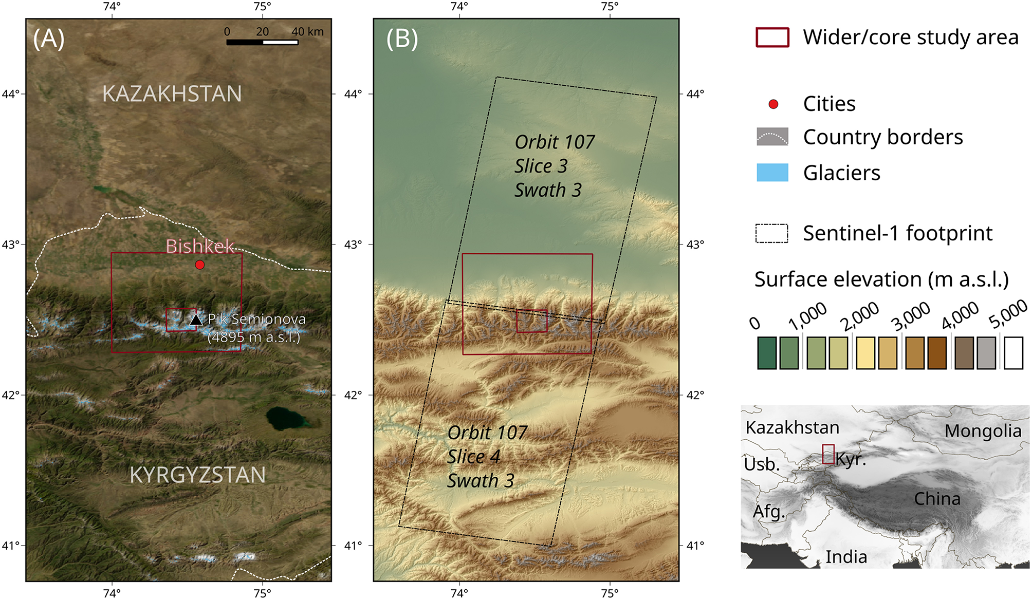
Overview of the case study region in the north-western Tien Shan mountain range. (A) Satellite image showing the distribution of vegetation, glaciers and the location of the city of Bishkek in the northern part of the study area. Satellite image from NASA Blue Marble, Glaciers from Randolph Glacier Inventory v6 (RGI Consortium, 2017). (B) SRTM-based topography and location of the Sentinel-1 scenes/swathes used in the study. The outer red box indicates the locations of the larger study area including the mountain front, alluvial fans, plains and the city of Bishkek; the inner box refers to the glacierized high-mountain core study area in the Ala Archa range (cf. Figure 2).
The study area also provides challenging conditions for S1 InSAR processing. The boundary between slices 3 and 4 of orbit 107 is located in the center of the region of interest. Topography at the northern slope of the Tien Shan is dominated by the contrast between rugged high mountain and lowland environments, accounting for relief >4,000 m. The core study area in the upper reaches of Ala Archa region (see Figure 1 for extent) represents a glacierized high-mountain environment with rugged topography (Figure 2). As such, it encompasses a variety of landforms that are susceptible to dynamic mass movement processes, such as deglaciated proglacial areas framed by Little Ice Age moraines, rock glaciers, steep slopes in permafrost-affected areas, and gullies (Figure 2).
Figure 2
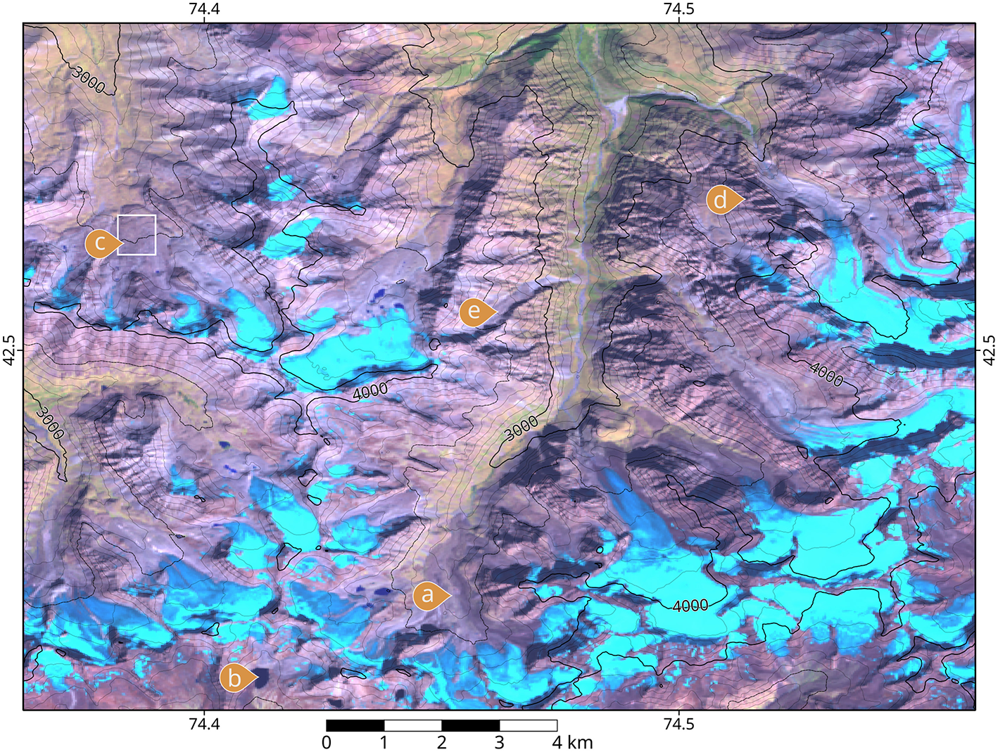
Core study area in the Ala Archa region of the Kyrgyz Range in optical imagery (Landsat 8, 2017-09-16, bands 6-5-4) with contours from SRTM. Arrows indicate features of particular interest, e.g., (a) proglacial areas framed by Little Ice Age moraines, (b) proglacial lakes, (c) rock glaciers, (d) steep slopes in permafrost areas, and (e) gullies. The white rectangle outlines the area investigated in the rock glacier coherence time series (cf. section 4.2).
2.2. Base Data and Processing Environment
Input data were limited to descending data takes from S1A and S1B. On descending orbits, the S1 satellites pass the study area in the night, at ~1 a.m. UTC and ~5 a.m. local time, respectively, so that these scenes are generally less affected by ionospheric disturbances than ascending data taken during the day. Besides this limitation, all available scenes from orbit 107, slices 3 and 4, were included. In order to obtain the maximum possible precision in interferometric processing, orbit parameterization was based exclusively on the “Precise Orbit Ephemerides” (AUX_POEORB) provided by the “Sentinel Payload Data Ground Segment” (https://qc.sentinel1.eo.esa.int/).
Processing was conducted on the “Cirrus” HPC cluster at Humboldt-Universität zu Berlin. Cirrus consists of one Login node (1 x Intel Xeon E5-2667v4, 8 cores, 64 GB RAM), eight basic compute nodes (each 2 x Intel Xeon E5-2640v4, 20 cores total, 64 GB RAM), and 12 high-memory compute nodes (each 2 x Intel Xeon E5-2640v4, 20 cores total, 128 GB RAM), so that a total of 400 cores and two TB RAM are available on the compute nodes.
3. Methods
3.1. General Software Design
OSARIS was designed with a focus on detecting short term changes in dynamic environments, particularly mountain ranges. Therefore, the core capabilities of the software are in pair-wise processing of a series of consecutive scenes to retain maximum temporal resolution, enabling researchers to investigate the timing, magnitude, and spatial extent of individual events. Conversely, detailed measurements of surface deformation on longer timescales by approaches that aim for geodetic precision, such as PSI, are not the primary goal of OSARIS. A special case in this regard are SBAS analyses, which are generally possible with GMTSAR but do hardly benefit from parallelization since GMTSAR conducts SBAS processing in a single process for all scenes.
Considering the minimalistic setup system administrators typically favor on processing nodes of HPC clusters, OSARIS was designed to require a minimum of software packages installed. Base software was chosen with focus on processing performance, exclusively using freely available open source products. These demands are best met by GMTSAR (see Table 1, Software assessment). GMTSAR bases on the “Generic Mapping Tools” (GMT; Wessel and Smith, 1991; Wessel et al., 2013), a library of C programs and Unix scripts for geocoded data, and therefore provides all routines necessary for pre- and post-processing. OSARIS combines these tools with the Slurm resource manager, providing a queuing and parallel processing environment for Linux-based HPC clusters. Conversely, Java, Matlab, and other higher languages were avoided for the above-mentioned reasons and the use of Python was restricted to a minimum in optional tools, e.g., to create plots and visualizations of results.
Table 1
| Name | Language | Based on | Open source | Accessibility | Scripting | PP-susceptibility |
|---|---|---|---|---|---|---|
| SNAP | Java | DORIS | Yes | Free | Python, shell | Native |
| GMTSAR | ANSI-C | GMT | Yes | Free | Shell | Multiple instances |
| ISCE | ANSI-C | ROI_PAC | Yes | Restricted access | Python | Unknown |
| GAMMA | ANSI-C | / | optional | Commercial | Native | Native |
| GiaNT | Python | Python modules | Yes | Free | Python, shell | Unknown |
| SARproZ | Matlab | Matlab modules | No | Restricted access | Unknown | Native |
Overview of SAR software products.
The core components of OSARIS are Bash shell scripts, providing easy integration in Linux/Unix environments, high performance, and convenient customization. In its current version OSARIS focuses on S1 scenes as input data; However, other sensors are supported by GMTSAR and may thus be implemented in the future.
For most scenarios, the setup can be conducted by editing two configuration template files according to machine configuration and processing demands (Loibl, 2019a). Configuration for system paths, input data, Slurm jobs, and general processing options, are merged in OSARIS' main configuration file template, which can conveniently be copied and fitted for individual processing projects. In cases where non-standard configurations regarding the interferometric processing are required, these can be tweaked in the GMTSAR configuration file.
OSARIS processes data in five steps (Figure 3): (i) Downloading input data; (ii) preprocessing; (iii) interferometric processing; (iv) post-processing, and (v) generating reports. Individual tasks which are to be performed in each step can be customized in the configuration file. This also allows skipping routines enabling users to split processing schemes into several phases. For example, it is often useful to start with a run performing only the preprocessing and interferometric processing steps, then check the results, and subsequently apply modules in separate runs. Processing steps which are implemented in Slurm-based parallel processing jobs are marked by [PP] in the following.
Figure 3
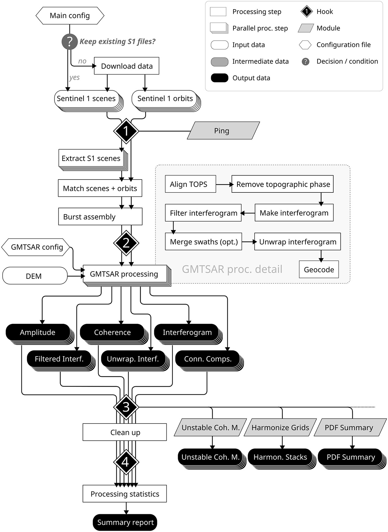
OSARIS processing scheme. The module setup presents an excerpt of key modules used in the case study (cf. section 3.3).
(i) Downloading of data is optional. OSARIS can also work with existing folders for both SAR scenes and orbits. This offers the opportunity to update the scene repository when new scenes become available, allowing repeated updates. When downloading is activated, OSARIS will use a shell script provided by ESA (dhusget.sh; https://github.com/SentinelDataHub/Scripts) to download S1 scenes based on relative orbit and latitude/longitude corner coordinates. Orbit data can either be in a local copy of the orbit repository which OSARIS will automatically update on each run or be downloaded on demand to reduce required disk space and download capacities. Appropriate digital elevation model (DEM) data must be supplied by the user and can, for example, be obtained using the online tool provided on the GMTSAR website (http://topex.ucsd.edu/gmtsar/demgen/).
(ii) Preprocessing comprises creation of directories and symlinks, extraction of S1 zip archives [PP], linking of S1 scenes and orbits, and creating list files of input files and related orbits. Optionally, unnecessary bursts can be cropped and the DEM can be cut to scene extent for improved efficiency. In case the area of interest is at the edge of two slices the relevant bursts will be extracted from both files and merged for further processing.
(iii) Interferometric processing is based on GMTSAR, using its tools to align scenes [PP], calculate coherence [PP], remove topographic phase [PP], filter phase [PP], process interferograms [PP], and unwrap phase with Snaphu (Chen and Zebker, 2000, 2001, 2002) [PP]. Two basic processing modes are available, “chronologically moving pairs” (A–B, B–C, C–D, […]) and “single master” (A–B, A–C, A–D, […]). In addition, OSARIS offers calculation of the difference of forward minus reverse interferograms (ϕAB − ϕBA) [PP] to identify unwrapping errors. In case multiple swaths are relevant, OSARIS will process each swath, merge the results, and crop them to the area of interest extent. All results are provided as stacks of geocoded grid files with a common naming scheme which includes the dates of master and slave scene (yyyymmdd) and the processing step(s), e.g., “20170729–20170810-coherence.grd.”
(iv) Most tasks in the post-processing phase are optional. Subsequently, a clean-up routine removes unnecessary and temporary data. The level of deleting is set in the main configuration file.
(v) OSARIS collects metadata of the executed processes. In the final phase, the meta data are written to report files that provide an overview of processing characteristics, e.g., total run time vs. wall clock run time.
3.2. Modules
After each processing step, interfaces to include additional routines, so-called hooks, are implemented. These hooks allow for the integration of modules in order to apply additional processing tasks to the data available at this point (Figure 3), facilitating to tailor processing schemes to specific goals. Module code must be supplied in the modules subdirectory of OSARIS. Modules need to be activated in the main configuration file and may supply additional configuration files. In the following, several core modules are described in detail. A comprehensive and regularly updated list is incorporated in the readme file (Loibl, 2019a).
3.2.1. Ping
Ping sends a series of minimal jobs to the Slurm queue in order to wake up nodes that are in stand-by mode. This ensures that the cluster is fully available at the time the GMTSAR parallel jobs are sent to the Slurm queue.
3.2.2. Stable Ground Point Identification (SGPI)
Identify stable ground by finding the pixel that exhibits the highest coherence throughout the time series
where γ is the coherence of each of the n pairs.
3.2.3. Harmonize Grids (HG)
Time series of raw unwrapped interferogram or line-of-sight displacement results typically exhibit substantial undesirable variability owing to different reference points for phase unwrapping. Since this is inevitable through the parallel and pair-wise application of GMTSAR and Snaphu, a posterior harmonization of unwrapping results is essential for higher level analysis. In standard configuration HG uses the coordinates of a “stable ground point” reference provided by a preceding SGPI run as input. Alternatively, the reference point coordinates can be provided manually. Assuming that the surface elevation change is zero at the reference point, the HG module identifies the value at the specified coordinates for each input dataset and then shifts the whole grid by the inverse value:
where Φunwr is the input grid file, e.g., unwrapped phase or Line-of-Sight displacement (LOSD), and ΦSGP is the value at the stable ground point location.
3.2.4. GACOS Correction
This module applies “Generic Atmospheric Correction Online Service for InSAR” (GACOS; Yu et al., 2017, 2018) data to correct unwrapped interferograms for signal delays originating from atmospheric disturbances. GACOS data acquisition currently needs to be performed manually via the web frontend (http://ceg-research.ncl.ac.uk/v2/gacos/); An API for automated data retrieval is announced and is planned to be implemented into the module upon release. The processing procedure follows the recommendations from the GACOS documentation (cf. Yu, 2017). First, the difference between the GACOS files is calculated for each pair of dates. Subsequently, the series of GACOS files are harmonized to a reference point, typically using the stable ground point identified by the SGPI module. In case the interferogram time series is not already harmonized to a reference point, these will also be harmonized to the same reference point. Ultimately, the correction is applied by subtracting the harmonized GACOS differences from the harmonized phase for each time step.
3.2.5. Unstable Coherence Metric (UCM)
UCM provides a coherence-based algorithm aiming to allow for the detection of surface changes in dynamic environments. Therefore, UCM does not rely on statistic properties of the whole time series but focuses on changes between two individual pairs of scenes. The module walks through the series of processed coherence files and, for each pair, identifies regions where high coherence values in the chronologically prior file coincide with a substantial coherence drop in the chronologically following file. Both high coherence and drop are defined by threshold values in the configuration file and may thus be fitted to the properties of specific environments (cf. section 3.3).
where γA and γB are two coherence files and UT and LT are upper and lower threshold values, respectively.
3.2.6. Detrend
The Detrend module fits low-order polynomial trends to a series of grid files using least-squares. Subsequently, the respective trend surfaces are subtracted from the individual grid files. Optionally, the trend files can be stored in a subdirectory for further analysis.
3.2.7. Statistics
This module calculates summary statistics for a series of grid files and returns a set of key statistical characteristics in a single csv file, including minimum and maximum values, median, scale, mean, standard deviation, and mode. The Statistics module can be configured to process several datasets in one run. Supplementary to the statistics module is the tool “pyStatisticPlot” that displays the results in a time series of boxplots.
3.2.8. Preview Files
GMTSAR's default scripts generate PNG images and Google Earth® KML files directly for each basic result file. This feature was moved to a module in OSARIS to provide users with more flexibility. The Preview Files module may thus be executed subsequent to higher level processing routines, limited to datasets that are actually of interest, or omitted when not needed. The module takes a list of one or more directories containing grid files as input and then renders the series of preview files to subdirectories. Generation of KML files is optional.
3.2.9. Summary PDF
The amount of individual image files in comprehensive time series of multiple InSAR datasets renders it challenging to obtain an overview. The Summary PDF module facilitates this by combining preview images of key processing results for each timestep in a single graphic overview (see Figure S1 for an example). By default, PDF Summary will display amplitude, coherence, unwrapped interferogram, and Snaphu connected components. However, the module can be configured to combine up to four of any of the results datasets available at the time when the module is called.
3.3. Specific Configuration
Configuration was set to process only swath 3 since it covers the entire area of interest. Cutting and merging was activated, so that only S1 bursts from slice 3 and 4 containing parts of the study area as provided by boundary box coordinates were processed into individual images. GMTSAR's filter wavelength was set to 100 m (default 200 m) to increase the resolution of results. The Slurm workload manager was configured to use 5 and 10 cores on the basic and high memory nodes, respectively, for individual parallel processing job to ensure sufficient RAM (i.e., ~30 GB per job). Such large amounts of RAM are required only by the phase unwrapping tool Snaphu in combination with high image resolution. Deactivating phase unwrapping or increasing the Gaussian filter wavelength substantially reduces the RAM requirement. Coherence thresholds for unwrapping and geocoding were set to 0.2 and 0.1, respectively. For interferometric processing, “chronologically moving pairs” mode with its A–B, B–C, C–D pattern was chosen for this demonstration, since the alternative “single master mode” processing scenes with its A–B, A–C, A–D pattern provides less coherence over the full dataset.
Seven key OSARIS modules were implemented to the workflow at different stages: (i) Ping, (ii) UCM, (iii) SGPI, (iv) HGS, (v) GACOS Correction, (vi) Detrend, and (vii) PDF Summary.
Ping was activated in the first hook, so that it is launched after file downloads and before pre-processing, triggering processing nodes to boot while S1 files are being extracted and preprocessed on the main node. In our setup, Ping saves about 3:30 min of runtime when nodes are in standby mode.
UCM is activated in the post-processing hook since it requires as input the coherence files processed by GMTSAR. A relatively low threshold value of 0.4 was chosen as high coherence threshold accompanied by a low value of 0.1 for the drop threshold taking into account the study's focus on high mountain environments.
The SGPI module identifies points that exhibit high coherence throughout the time series. In this case study, we used the module “Crop” previous to SGPI to cut the unwrapped interferogram and LOSD time series to the extent of the core study area. This ensures that the result is relevant for the region under investigation. Subsequently, the SGPI module was then configured to solely return the coordinates of the point with highest average coherence which could then to be used as “stable ground” reference point in the following processing step.
Using the stable ground point identified by the SPSI module, the HG module measures the value at this point in each unwrapped interferogram in the time series. Each file is then shifted so that the value at the stable ground point is zero. The harmonized time series then allows for comparative analysis between individual time steps.
The imprints of atmospheric signal delays in unwrapped interferograms are corrected using GACOS data (cf. section 3.2.4).
Subsequent to processing, PDF Summary generates a single document providing overview maps of the the key processing results coherence, amplitude, connected components, and LOSD.
3.4. Comparison to ISCE and SNAP
In order to evaluate whether the quality of OSARIS results is competitive despite its high level of automatization, a comparison to results from two other state-of-the art InSAR software tools, ISCE (Rosen et al., 2012) and SNAP (ESA, 2018), was conducted. However, processing a similar time series would be extremely laborious or not feasible in ISCE and SNAP, respectively. Therefore, the comparison had to be restricted to selected scene pairs. Out of the S1 data available for the case study area, one pair of particularly challenging (2016-11-25 to 2016-12-19) and one of particularly expedient (2017-07-29 to 2017-08-10) processing conditions, i.e., low and high coherence, were chosen. For these scene pairs, coherence and unwrapped interferograms were obtained with each software, so that one fundamental and one higher level dataset could be compared. Notably for OSARIS in this context, these fundamental InSAR datasets for individual scene pairs are basically GMTSAR results. However, the quality of these datasets strongly depends on configuration and preprocessing routines, particularly merging of slices, burst assembly and orbit processing, all of which are conducted automatically by OSARIS. Therefore, the comparison aims to test the performance of OSARIS as a specific, highly automatized GMTSAR implementation. All results were cut to the same boundary box extent (upper left: 74E/42.8N, lower right: 74.7E/42.3N) and unwrapped interferograms were harmonized to their respective medians to facilitate comparison between different processors.
Since each software applies different algorithms and filters, configurations were fitted for best inter-comparability. For example, GMTSAR/OSARIS uses a Gaussian Filter instead of the multilooking of ISCE and SNAP. We chose a pragmatic approach to manage these differences and retain the processing characteristics of each tool by configuring individual processing chains for a target resolution of ~30 m in the unwrapped interferograms. One arc second (~30 m) SRTM DEMs were consistently used for topographic phase removal by all tools. All three tools use Snaphu for phase unwrapping by default. However, SNAP does not include Snaphu in the main processing routines but requires manual export before and re-import after phase unwrapping. As outlined in Chapter 3.1, merging of slices 3 and 4 of orbit 104 is required to process the study area.
For robust comparison of the resulting raster files we apply the SPAtial EFficiency metric (SPAEF; Koch et al., 2018), which combines three equally weighted statistic parameters:
where α is the Pearson correlation coefficient (CC) between reference (OSARIS) and compared raster (ISCE, SNAP), β is a ratio of the coefficients of variation (CVR) representing spatial variability, and γ is the histogram intersection (HI) for the given histogram K of the reference raster and the histogram L of the compared raster, each containing n bins.
4. Results
In the following the results from the case study will be presented, aiming to provide insights into key features and capabilities of the OSARIS framework. Please note that the presentation had to be limited to overviews and individual examples owing to the vast amount of result datasets. An archive of key result time series datasets in grid file format (~18 GB) is available via the “GFZ Data Services” repository (Loibl, 2019b).
4.1. Data Characteristics
During the run on May 5, 2019, a total of 174 S1 scenes (622 GB) were retrieved automatically from ESA's DHUS hub, covering a timespan from January 17, 2015 to April 26, 2019, for slices 3 and 4 of orbit 107 (Table S1). After slice merging and cutting to the study area extent, a total of 81 files were available for interferometric processing, resulting in 80 pairs of scenes. Omission of scenes was caused by two reasons: a change of slice extents by ESA in late 2015 that lead to failures in the cut and merge procedure (n = 7), and missing precise orbits for the newest acquisitions (n = 4, two dates).
Interferometric processing provides amplitude, coherence, interferometric phase, and unwrapped phase for each pair of scenes. Results are stored as geocoded grid files. Setting GMTSAR's filter wavelength to 100 m yielded a resolution of ~31 m for each grid file. The series of unwrapped interferograms was subsequently harmonized to a common reference point through the application of the SGPI and HG modules, facilitating comparison throughout the stack. Correction for atmospheric signal delays and large-scale trends was conducted using the GACOS correction and Detrend module, respectively.
Wall clock processing time was 12 h 3 min 58 s (excluding S1 scene download time). The total time including parallel jobs amounted to 12 d 22 h 48 min, indicating ~12 d 10 h 44 min (~96%) were saved through parallelization. Considering individual processing steps, the largest part of processing time, 11 d 10 h 58 min 52 s (wall clock time 9 h 33 min 41 s), was consumed by interferometric processing (cf. step iii in section 3.2). With 1 d 1 h 11 min 50 s (wall clock time 2 h 17 min 5 s) modules had the second largest share of processing time, followed by extraction of S1 archives with 10 h 27 min 12 s (wall clock time 1 h 2 min 44 s). The remaining ~10 min encapsulate all other routines, including preprocessing, file operations, clean up, and reporting.
Total disk space requirement was ~2.5 TB. Out of this, the majority of ~1.8 TB is located in the “Processing” directory for temporary files that may be deleted afterwards or removed automatically during the run through the “Clean up” parameter in the configuration file. Input files, i.e., the zipped S1 files, amount to 622 GB. The “Output” directory containing all result files has a total size of 49 GB. The latter includes, however, several interim stages of the module processing chain which may also be omitted. The basic interferometric processing results before applying modules total to ~24.5 GB. The “Log” directory contains another 221 MB of text files documenting the run.
4.2. Amplitude and Coherence
Amplitude and coherence of interferometric SAR datasets are valuable measurements useful for change detection and have been applied to a wide range of features, including aeolian landforms (Wegmuller et al., 2000; Liu et al., 2001; Havivi et al., 2017), flood detection and fluvial channel dynamics (Nico et al., 2000; Ullmann et al., 2019), and infrastructure change/damage (Liao et al., 2008; Nakmuenwai et al., 2016). OSARIS generates comprehensive time series of both amplitude and coherence (Figure 4, Figure S1) and provides modules to facilitate further analysis (cf. section 4.4).
Figure 4
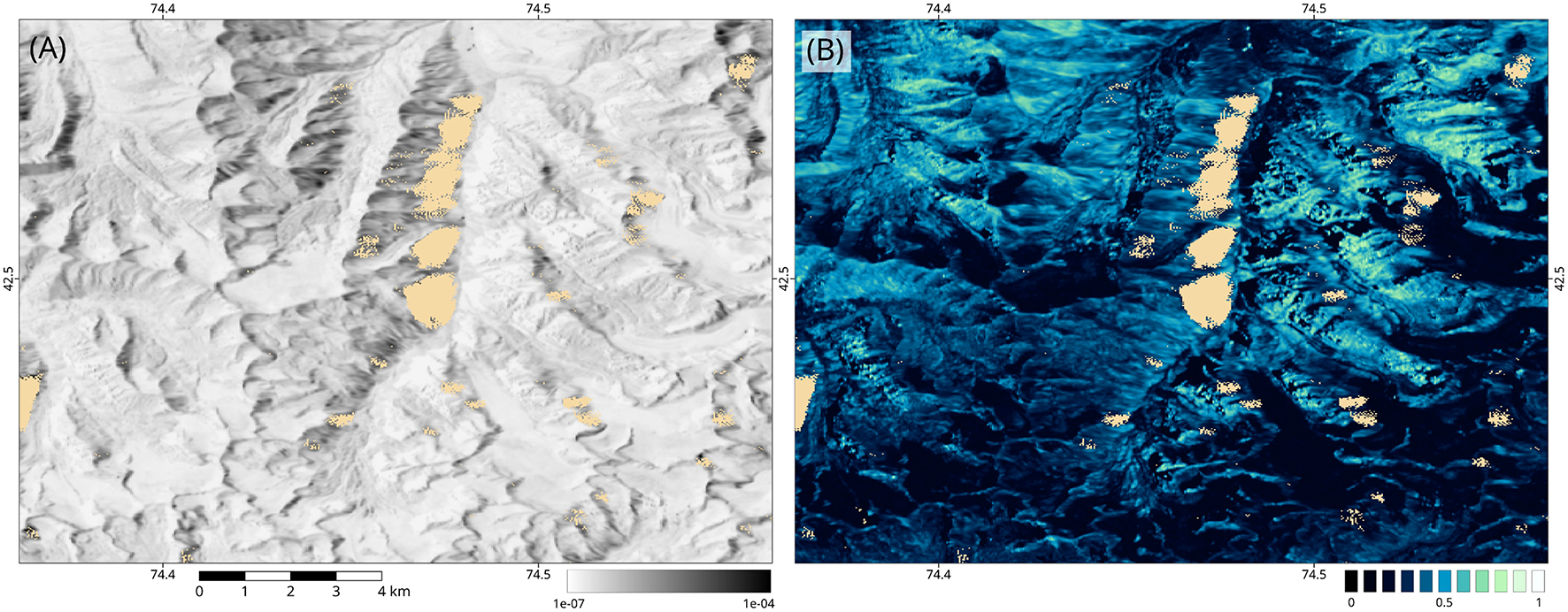
Average (A) amplitude and (B) coherence values for the full time series (n = 54) and the core study area in the Ala Archa mountain range (cf. Figure 2). Beige color indicates locations where at least one result had “no data” values. Contains modified Copernicus Sentinel data 2015–2019.
Average amplitude distinctly correlates with topography, with relatively high values on ridges and slopes facing away from the sensor, i.e., approximately toward the East, and low values on slopes facing toward the sensor as well as on relatively flat terrain (Figure 4A). Average coherence is highest on spurs and ridges with maximum values of ~0.85. Conversely, low average coherence values < 0.3 prevail over glaciers, slopes steeper ~45°, gullies, and talus cones (Figure 4B). “No data” values occur predominantly on steep slopes facing away from the sensor, indicating interferometric processing results in these areas should be treated with caution or masked.
The coherence time series exhibits strong seasonal variability (Figure 5). April is consistently the month with lowest monthly average median coherences of ~0.2 for all three investigated settings. From spring to late summer, coherence values exhibit increasing trends in each series and for each year, with maximum monthly average median coherences reaching ~0.52, ~0.61, and ~0.75 in the wider study area (Figure 5A), Ala Archa (Figure 5B), and rock glacier (Figure 5C) settings, respectively. This shows that, consistent with expectations, the variability is more pronounced in the high mountain environment of the core study area than in the wider region where different dynamics of snow, vegetation, moisture, etc., tend to offset each other. Backscatter at the rock glacier site is controlled by the contrasting reflective properties of snow and rock, leading to extreme differences of ~±0.6 median coherence between winter/spring and summer. In the mountain environment, coherence drops significantly (~−0.5) during autumn each year as a consequence of the first snowfall. The highest variability in coherence between individual consecutive pairs and between 2016 and 2017 occurs during winter and spring, presumably caused by changes in moisture, snow cover, and vegetation.
Figure 5
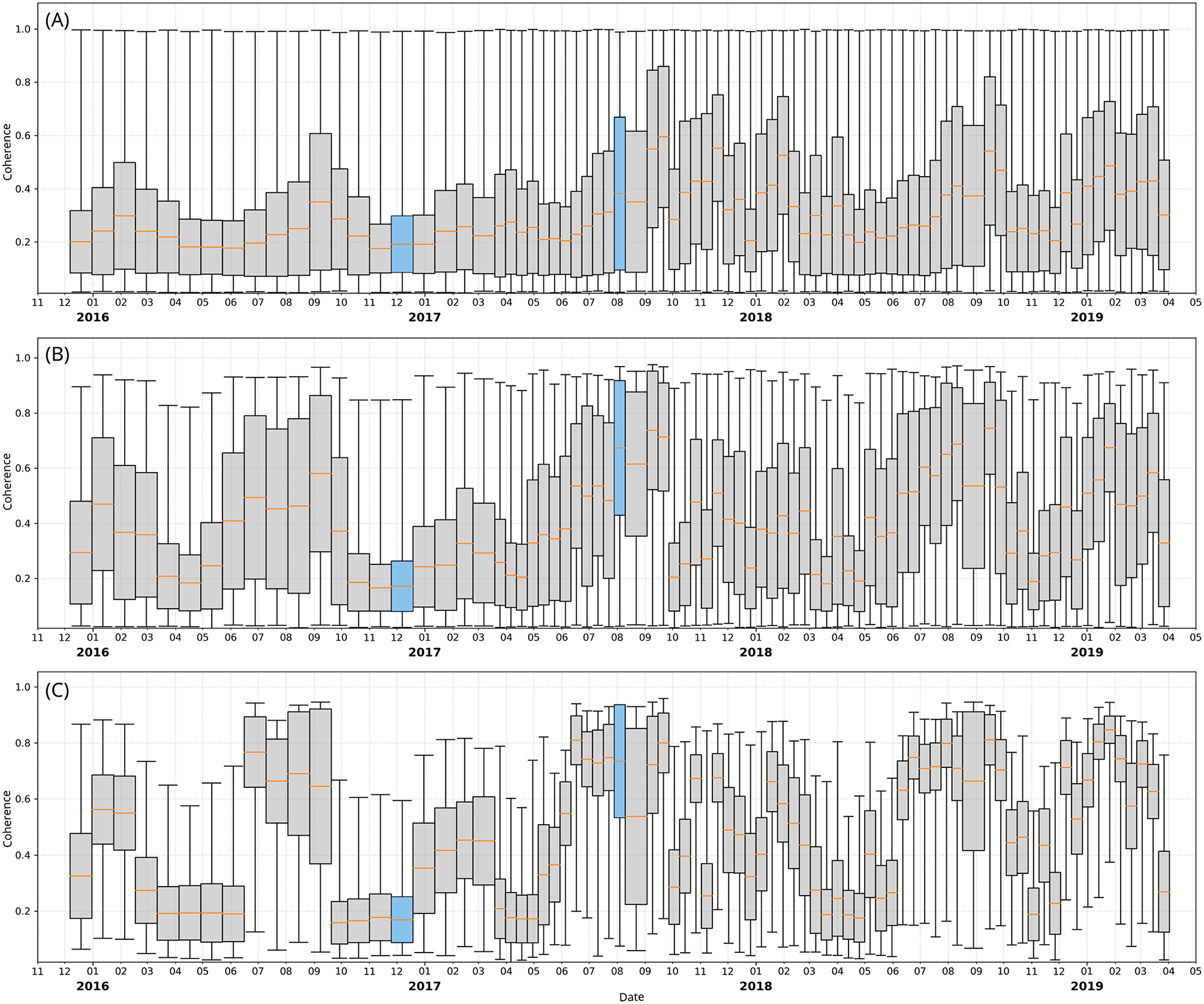
Box plots of OSARIS coherence processing results for the full time series and (A) the wider study area, (B) the core study area in the Ala Archa mountain range, and (C) a rock glacier as example for an individual landform (cf. Figures 2, 4). Box width shows the timespan covered by individual scene pairs. Blue colors mark the time steps (2016-11-25 to 2016-12-19 and 2017-07-29 to 2017-08-10) that are investigated in more detail in the subsequent figures. The figure was generated using OSARIS' “pyStatisticPlot” based on output of the “Statistics” module. Contains modified Copernicus Sentinel data 2015–2019.
The high coherence pair example (2017-07-29 to 2017-08-10) for the wider study area reveals substantial heterogeneity (top row in Figure 6). High coherence values > 0.7 are abundant in the higher alpine and nival levels, individual slopes in the foothills at the fringe of the mountain range, individual agricultural fields, and settlements. Conversely, low coherence < 0.3 prevails over glaciated areas, throughout the subalpine and montane zones as well as on the alluvial fans. The detail from the mountain range (bottom row in Figure 6) highlights the distinct coherence contrast between glaciers (< 0.2) and adjacent bare rock surfaces (> 0.7). Steep, east facing slopes exhibit conspicuous stripe patterns often accompanied by data gaps, indicating signal shadows on inclined surfaces facing away from then sensor.
Figure 6

Coherence example results for the (A,B) wider and (C,D) core study area. (A,C) Show data for the high coherence pair 2016-11-25 to 2016-12-19, (B,D) for low coherence pair 2017-07-29 to 2017-08-10. Contains modified Copernicus Sentinel data 2016, 2017.
4.3. Unstable Coherence Metric (UCM)
The UCM module aims to facilitate automatized detection of change events as well as to provide a measure for their magnitude. A time series of coherence changes is used as input for UCM. Figure 7 shows an excerpt from the UCM time series for the core study area covering the time span 2017-07-05 to 2017-10-09. Since UCM considers coherence from two consecutive pairs of scenes (cf. section 2.2), each UCM image involves three data takes (e.g. 2017-07-05, 2017-07-17, 2017-07-29 for Figure 7A) with the middle data take being slave in the first and master in the second pair (e.g., 2017-07-17 for Figure 7A). High UCM values indicate a substantial drop from high to low coherence values between the two scene pairs, implying that change occurred on a surface that was stable and well-reflecting in the earlier scene pair. Such events are abundant on slopes in permafrost areas and in proglacial settings, including Little Ice Age moraines, rock glaciers, glaciofluvial, and glaciolimnic features.
Figure 7
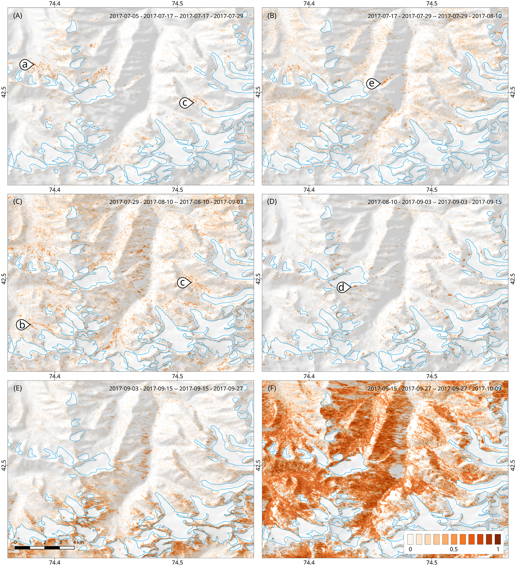
Excerpt of “Unstable Coherence Metric” processing results covering the timespan 2017-07-05 to 2017-10-09 (A–F). High UCM values indicate areas of significant loss of coherence between two consecutive pairs of scenes. Regions in white to grey colors (hillshade) represent no-data UCM values. Arrows highlight examples of high UCM values that relate to specific landforms of interest: (a) rock glaciers, (b) Little Ice Age moraines, (c) proglacial areas, (d) steep slopes in permafrost areas, and (e) gullies. A semitransparent hillshade based on SRTM DEM data and glacier outlines from Randolph Glacier Inventory v6.0 were added for orientation. Contains modified Copernicus Sentinel data 2017.
The time series from July to October 2017 reveals that substantial activation of surface movement processes occurred during the summer months, with particularly strong and widespread events during late July and August. Distinct phases of activity for individual landforms can also be observed. For instance, the rock glacier highlighted by arrow (a) in Figure 7A displays high UCM values during July and August (Figures 7A–C) and significantly lower values in the consecutive results (Figures 7D,E). Conversely, pronounced local events that focus on ridges and slopes in permafrost areas are abundant in the period from late August to early September (Figure 7D). During September, UCM values exhibit two altitudinal belts, with low values prevailing in the lower and high values in the higher portion of the scene, presumably caused by snowfall (Figure 7E). A large-scale coherence drop dominates the UCM result of late September–October (Figure 7F), indicating extensive snowfall (cf. Figure S2).
4.4. Line-of-Sight Displacement
Datasets derived from interferometric phase, such as LOSD, are subject to various natural and processing-related factors, such as atmospheric moisture content, ionospheric disturbances, changes in vegetation, and the influence of DEM errors during removal of topographic phase. These may adversely affect the results, demanding masking of artifacts and correction of specific effects. In the following, the capabilities of OSARIS for creating automatic processing chains to correct comprehensive stacks of LOSD data are demonstrated. For illustration, a high coherence scene pair, 2018-08-05 to 2018-08-17, was selected (Figure 8). Notably for this dataset, raw LOSD displacement processing results already show widely consistent patterns even in the high-mountain core study area (Figure 8A). This excludes the aforementioned regions of prevailing low coherence, i.e., glaciers and steep east-facing slopes, which are characterized by patchy extreme values and striped artifacts, respectively. OSARIS facilitates masking regions of deficient phase unwrapping using sums of forward plus reverse pair unwrapping (Figure 8C). The resulting dataset exhibits less noise and several distinct features have been removed (e.g., marker f in Figures 8A,D). In the wider study area, however, a distinct imprint of topography is still evident, typically caused by atmospheric disturbances affecting the SAR signal. These are subsequently corrected using GACOS data (cf. section 2.2), resulting in a much smoother overall image (Figure 8H). Remaining large-scale gradients are treated using the Detrend module which calculates a best-fit polynomial surface for correction (Figure 8I). Notably, the core study area is hardly affected by the GACOS correction and Detrend routines (Figures 8G,J).
Figure 8
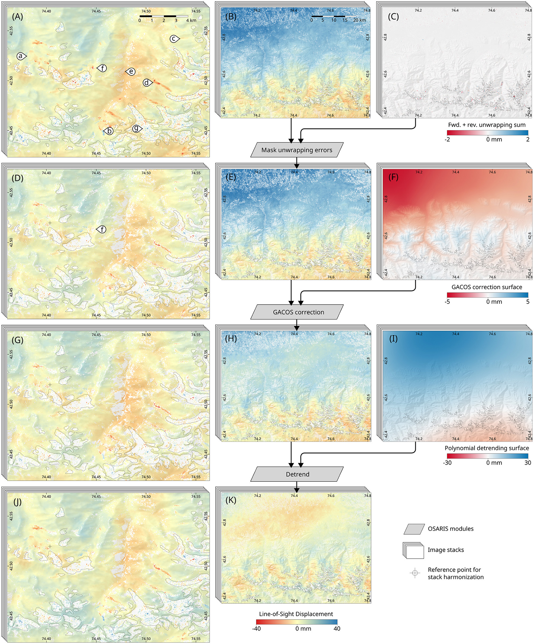
Example processing chain for Line-of-Sight displacement (LOSD) results, demonstrated with the scene pair 2018-08-05 to 2018-08-17. Left and middle columns show results for the core and wider study area, respectively. The right column presents supplementary datasets that are used in the next processing step. (A,B) Harmonized LOSD dataset and (C) forward plus reverse pair unwrapping sums which are used to mask phase unwrapping errors. (D,E) Masked LOSD and (F) GACOS correction surface which is used to correct for atmospheric signal delays. (G,H) LOSD after GACOS correction and (I) polynomial surface used to remove large-scale trends. (J,K) LOSD after trend removal. Note that each processing step was automatically applied to the whole stack. Markers in (A) indicate (a) a rock glacier, (b) a Little Ice Age moraine ridge, (c) a gully, (d) a proglacial drainage channel, (e) striped artifacts, (f) a region of deficient phase unwrapping that was masked in (D), and (g) patchy extreme values over a glacier. A semitransparent hillshade based on SRTM DEM data and glacier outlines from Randolph Glacier Inventory v6.0 were added for orientation. Contains modified Copernicus Sentinel data 2018.
Several distinct features remain after the masking and correction procedures, and confidence is thus high that these are depicting real displacements. Specifically, patterns of deformation along multiple channels in proglacial areas, gullies on slopes, and moraine ridges, are consistent in spatial extent in individual scenes and with expectations regarding the geomorphological process systems. These patterns often prevail throughout multiple scenes in the time series (Figure S1).
4.5. Comparison to ISCE and SNAP
The results of the InSAR processing tool comparison based on the SPAEF metric (section 2.3) are provided in Table 2, histogram and scatter plots illustrating the underlying data are incorporated in Figure 9. The differences between OSARIS and ISCE coherence results reveal that ISCE generates substantially higher overall coherence/topophase correlation (Figures 9A,B). Particularly for 2016-11-25 to 2016-12-19, histograms show similar distribution curves but a distinct shift toward higher values in ISCE, leading to the lowest HI value of ~0.45. Spatial patterns of distribution for the high coherence pair 2017-07-29 to 2017-08-10 (Figure 9B) indicate that ISCE's coherence results are higher than those of OSARIS and SNAP, particularly in regions of relatively low coherence and challenging sensing conditions, such as glaciated surfaces, vegetated areas, and steep slopes facing away from the sensor. In addition, the bimodal histogram curves exhibit a clear trend toward higher ISCE absolute coherence values in the range > 0.8. This is also evident in a distinct cluster at high ISCE coherence values in the scatter plot. Statistically, the general similarity of spatial and absolute value distribution lead to relatively high CC (~0.72) and HI (~0.87) values, respectively. Conversely, the deviations at the higher and lower portions of the value range are reflected by a relatively low CVR value of ~0.64, resulting in an intermediate SPAEF of ~0.52. Interestingly, OSARIS exhibits higher coherence values on ridges whereas ISCE along valley bottoms, steep slopes, and over glaciers.
Table 2
| Dataset | Dates | References | Comparison | SPAEF | CC | CVR | HI | References Figures |
|---|---|---|---|---|---|---|---|---|
| Coherence | 20161125-20161219 | OSARIS | ISCE | 0.0593 | 0.4877 | 0.4379 | 0.4463 | Figure 9A |
| Coherence | 20161125-20161219 | OSARIS | SNAP | 0.5556 | 0.6405 | 0.7787 | 0.8610 | Figure 9C |
| Coherence | 20170729-20170810 | OSARIS | ISCE | 0.5241 | 0.7180 | 0.6391 | 0.8705 | Figure 9B |
| Coherence | 20170729-20170810 | OSARIS | SNAP | 0.8483 | 0.8843 | 0.9083 | 0.9649 | Figure 9D |
| Unwr. Interf. | 20161125-20161219 | OSARIS | ISCE | −3.1167 | 0.3594 | −3.0649 | 0.8837 | Figure 10A |
| Unwr. Interf. | 20161125-20161219 | OSARIS | SNAP | −1.3883 | 0.2191 | −1.0983 | 0.1686 | Figure 10C |
| Unwr. Interf. | 20170729-20170810 | OSARIS | ISCE | 0.6566 | 0.7783 | 0.7389 | 0.9765 | Figure 10B |
| Unwr. Interf. | 20170729-20170810 | OSARIS | SNAP | 0.7066 | 0.7218 | 0.9102 | 0.9761 | Figure 10D |
SPAtial EFficiency metric (SPAEF) results.
Figure 9
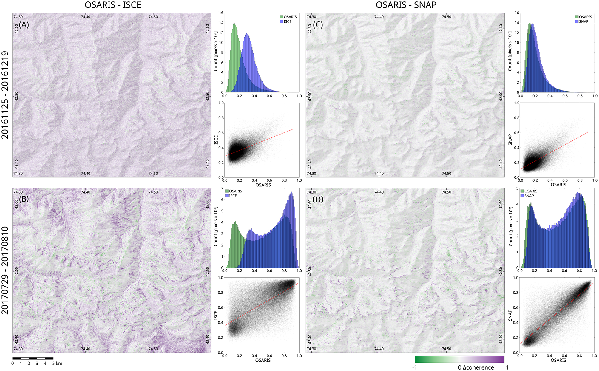
Differences in coherence and corresponding SPAtial Efficiency metric results (histograms, scatter plots) for the core study area. (A) OSARIS—ISCE for the low-coherence pair 2016-11-25 to 2016-12-19, (B) OSARIS—ISCE for the high-coherence pair 2017-07-29 to 2017-08-10, (C) OSARIS—SNAP for the low-coherence pair 2016-11-25 to 2016-12-19, (D) OSARIS—SNAP for the high-coherence pair 2017-07-29 to 2017-08-10. Difference images for the wider study area are available in Figure S3, the respective coherence results from the individual processors in Figure S4. A semitransparent hillshade based on SRTM DEM data was added for orientation. Contains modified Copernicus Sentinel data 2016, 2017.
Similar to ISCE, SNAP's coherence results for the pair with adverse processing conditions, i.e., 2016-11-25 to 2016-12-19, exhibits a similar pattern of histogram distribution as OSARIS, with a shift of ~+0.05 toward higher values (Figure 9C). The total differences are thus of smaller magnitude than with ISCE, leading to relatively high CVR and HI values of ~0.78 and ~0.86, respectively. The high coherence pair 2017-07-29 to 2017-08-10 (Figure 9D) exhibits the best match of all coherence datasets, with a SPAEF of ~0.85 owing to high values in CC (~0.88), CVR (~0.91), and HI (~96). The histogram shows that OSARIS' coherence result tends to more extreme values than SNAP, i.e., more values in the ranges < ~0.15 and > ~0.85. Spatially, extremes in Δcoherence between OSARIS and SNAP focus on ridges and steep slopes facing away from the sensor, with a clear dominance of higher SNAP coherence values on ridges and alternating patterns between different slopes.
Despite ISCE's substantially higher coherence values under adverse processing conditions, ISCE's unwrapped interferograms for the 2016-11-25 to 2016-12-19 scene pair show few differences to OSARIS' results for a substantial portion of the mountain range (Figure 10A). Consequently, the histograms also exhibit clear similarity (HI ~0.88) with the exception of a slightly higher abundance of negative values in the range ~−18 to −6 in the ISCE result. However, in the northern and particularly in the southern part of the detail high Δ values > ±5 prevail, owing to unwrapping-specific artifacts such as local errors and connected component boundaries (cf. Figure S6). These pronounced local divergences are clearly systematic as visible in diagonal patterns in the scatter plot of Figure 10A and lead to the lowest CC, CVR and SPAEF values of ~0.36, ~−3.06 and ~−3.12, respectively. The difference image for OSARIS—SNAP unwrapped interferograms (Figure 10C) is dominated by patches of strong positive and negative values. SNAP's multimodal histogram clearly indicates that the dataset is affected by substantial breaks in the distribution of phase unwrapping connected components, resulting in the lowest overall HI of ~0.17. For the high coherence pair 2017-07-29 to 2017-08-10 good agreement between results from all three tools was achieved, except for low coherence regions such as glaciers and presumably active landforms such as proglacial areas and talus cones.
Figure 10
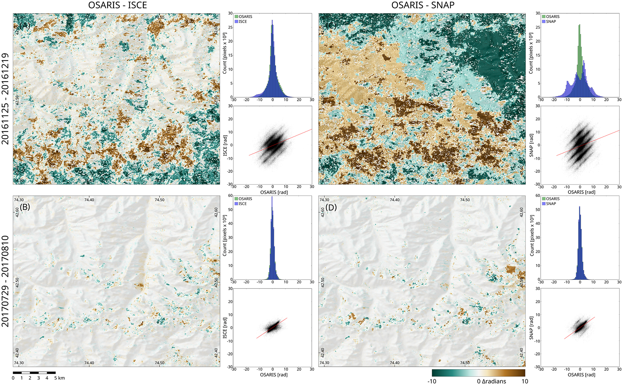
Differences in unwrapped interferograms and corresponding SPAtial Efficiency metric results (histograms, scatter plots) for the core study area. (A) OSARIS—ISCE for the low-coherence pair 2016-11-25 to 2016-12-19, (B) OSARIS—ISCE for the high-coherence pair 2017-07-29 to 2017-08-10, (C) OSARIS—SNAP for the low-coherence pair 2016-11-25 to 2016-12-19, (D) OSARIS—SNAP for the high-coherence pair 2017-07-29 to 2017-08-10. Difference images for the wider study area are available in Figure S5, the respective coherence results from the individual processors in Figure S6. A semitransparent hillshade based on SRTM DEM data was added for orientation. Contains modified Copernicus Sentinel data 2016-2017.
In summary, ISCE provides the highest coherence values in all test cases, with the most prominent deviations (Δ > 0.3) in scene pairs (Figure 9A) or sub regions (Figure 9B) with challenging sensing conditions. Despite a slight trend toward higher values visible in the histograms (Figures 9C,D), coherence values obtained by SNAP show strong similarity to those of OSARIS/GMTSAR, particularly regarding overall value frequencies and patterns of spatial distribution, as evidenced by CVRs of > 0.77 and HIs > 0.86. Notably, the coherence processing algorithms of SNAP and particularly ISCE (topophase correlation) are different from GMTSAR, so that the absolute coherence values do not allow for general inferences regarding the quality of the tools' processing results. Nevertheless, the Δcoherence provides a valuable indicator of how well individual tools handle specific challenges as outlined above. This point is supported by the comparison of unwrapped interferograms, where HIs of ~0.88 and ~0.98 highlight the dominating similarities between the results of ISCE and OSARIS. CVRs of ~−3.06 and ~0.74 are indicating the pronounced local deviations between the unwrapped interferograms of OSARIS/GMTSAR and ISCE, particularly under challenging conditions. Notably, in contrast to SNAP, OSARIS' and ISCE' unwrapped interferograms still allow to distinguish between unwrapping artifacts in such cases, so that automated masking routines may be applied.
5. Discussion
5.1. Setup and Processing
Scenes before 2015-12-07 (n = 7) failed in processing, owing to a different configuration of the slice extent. An automatic routine for this issue is planned to be implemented in OSARIS in the near future. With the current version this could easily be solved by processing all swaths or by cutting and merging the scenes manually. However, we decided to refrain from any interventions to the general workflow to provide a genuine demonstration of OSARIS' functioning and its high level automatization. In combination with the template-based configuration concept, this saves a substantial amount of time in comparison to other available software tools or manual configuration of GMTSAR routines, particularly for comprehensive time series. The benchmarks presented in Chapter 4.1 show that parallelization reduced processing time by ~96%. Notably, the HPC cluster setup used was not sufficient to run all 80 interferometric processing jobs at the same time. Therefore, wall clock processing time could be reduced further if more CPU cores and/or RAM per core were available. The total hard disk storage requirement of ~2.5 TB may be reduced to a minimum of ~49 GB by activating the most thorough clean-up option, which will only retain result and log files.
5.2. Evaluation of Case Study Results
The coherence time series (Figures 4–6, Figure S3) and the comparison to results from other state-of-the-art SAR processing software, i.e., ISCE and SNAP (Figure 9, Figure S3), demonstrates that OSARIS' routines for SAR preprocessing and scene alignment yield results of competitive quality. The comparison to ISCE and SNAP also allowed for identification of specific strengths and weaknesses of each processor. Specifically, ISCE generates higher coherence values under adverse conditions. Nevertheless, except for a general trend of ISCE to “smoother” results unwrapped interferograms from OSARIS and ISCE exhibit highly similar distributions of values as evidenced by HI values of ~0.88 and ~0.98 for the low and high coherence pair, respectively. As such, it is well possible that the observed differences are rather a consequence of different approaches to calculate coherence as well as different filtering/multilooking routines applied. Regarding OSARIS and SNAP the results exhibit similar characteristics under favorable conditions. However, lacking features to process large stacks of data and the missing integration of phase unwrapping pose substantial obstacles for automated processing of comprehensive S1 datasets with SNAP.
Striped artifacts originating from deficient assembly of S1 TOPS bursts—common source of error in S1 TOPS processing products—are rare throughout the OSARIS' result dataset (Figure S3). Considering the heterogeneous and often challenging processing conditions in the case study area, differences between individual time steps in OSARIS coherence can be clearly attributed to specific changes of surface reflectance characteristics caused, for example, by snowfall, vegetation, glaciers, or surface moisture. Seasonal changes and the time interval between subsequent S1 data takes affect substantially coherence in the high mountain environment of the core study area (Figure 4).
5.3. Evaluation of Higher-Level Processing Results
Besides the straightforward correlation to coherence, OSARIS-derived interferograms are also consistent both internally and in comparison to results from other processing software (Figure 10, Figure S6). For high-coherence regions, LOSD results provide first-order estimates of movement rates. However, absolute values must be treated with caution owing to the sensitivity of pair-wise processing to various disturbances outlined before (Figure 8A). Forward-reverse unwrapping sums and Snaphu's connected components facilitate identifying and masking areas affected by unwrapping errors (Figures 8B,C). In combination with adequate low coherence thresholds for phase unwrapping, these datasets allow limitation of subsequent analyses of LOSD to regions where confidence in the quality of results is high. Notably, the effect of the correction modules GACOS and Detrend is very limited in the core study area, affirming the robustness of the obtained LOSD measurements in the vicinity of the reference point to which the time series is harmonized. These processing steps may thus be considered optional in cases where relatively high coherence prevails throughout the time series and the area under investigation is of limited spatial extent. It is thus advisable to base decisions regarding the implementation of these optimization modules on a survey of the properties of the whole time series, e.g., as provided by OSARIS' PDF Summary and Statistics modules. Furthermore, several images are affected negatively by the GACOS correction routine, e.g., by increases of large-scale gradients or newly introduced local disturbances, demanding a posterior evaluation of the effectiveness of this routine.
The UCM module provides a versatile tool to identify locations and timing of changes to objects of relatively high coherence, potentially indicating actual mass movement events as demonstrated for periglacial and proglacial features in Figure 7. In this example, the observed patterns are consistent with expectations that thaw- and melt induced instabilities occur on a variety of glacier- and permafrost-related landforms, such as potentially ice-cored Little Ice Age moraines or steep rockwalls in permafrost areas. However, a flexible threshold value configuration allows for applications of UCM in various scenarios, e.g., detecting river bank collapses or constructions affected by catastrophic events. Since UCM is based on coherence, it complements phase-based datasets very well. Specifically, UCM is less prone to measurement errors and hardly dependent on the satellite's looking angle. Nevertheless, substantial coherence drops may also be caused by other events, out of which snowfall and vegetation changes are of particular relevance in high mountain regions. Therefore, the spatial patterns of UCM results must be considered carefully in interpretations.
5.4. Prospects and Limitations
The main drawback of the OSARIS approach, particularly in comparison to GUI solutions like SNAP, is a lack of flexibility and interactivity in the processing procedure. Specifically, all configuration must be set up before executing the script, possibilities to review the results during the processing phase are limited, and changes to the setup in many cases require restarting the processing. It is therefore advisable to start a new OSARIS project with a small subset of S1 scenes and optimize the configuration before launching a comprehensive job. Options to use previously downloaded or existing extracted files as input data support this workflow of configuration optimization. Additionally, activating the options to skip preprocessing and/or interferometric processing facilitates using existing processing results and thus allows for effective tuning of the module configuration. In case a dataset requires substantial parameter tuning for individual scenes, the open structure and accessible data format of OSARIS allows for workflows that exploit OSARIS' parallel processing capabilities to generate fundamental SAR and InSAR datasets and subsequently import the data, e.g., into a GUI-based tool, for manual optimizations.
Users will need to have at least basic skills working with Unix shells to handle and optimize the processing; however, comments and hints are included throughout the scripts and outputs to keep such obstacles to a minimum. In addition, the documentation in the Github repository explains all steps required to install, configure and launch OSARIS, and a step-by-step tutorial is available on the CryoTools website (https://cryo-tools.org/osaris-tutorial-1). Ultimately, a HPC cluster with the workload manager Slurm is required to exploit OSARIS' parallel processing capabilities. Users who do not have access to such a computing environment may use cloud-based services. A regularly updated list of Slurm-enabled HPC cloud services including links to relevant resources is included in the OSARIS documentation.
OSARIS has its strongest advantages in studies aiming to obtain interferometric data from comprehensive series of S1 data in which retaining the full temporal and high spatial resolution is critical. For SAR processing experts, the shell file-based setup, modular structure and open source code provides many possibilities for fine-tailored, individual processing solutions. In this context we would like to point out that the images shown in the result section, particularly Figures 6–8, are limited to presenting individual examples out of 15 different full datasets, most of which contain 80 images covering the whole time series from December 2015 until April 2018. Despite substantial design efforts, it is impossible to represent such a dataset comprehensively in the format of figures in a scientific paper.
The case study from the Tien Shan mountains demonstrates the software's capability to obtain various information on location, timing and magnitude of surface displacement events in a dynamic high mountain environment. OSARIS' high degree of automatization facilitates processing large amounts of data in relatively short time and with reasonable configuration efforts. The comparison to ISCE and SNAP showed it is possible to implement a similar processing scheme for an individual scene pair and selected datasets, i.e., coherence and interferometric phase, with results of similar quality. However, setting up a scheme to process all datasets provided by OSARIS for the whole time series would have been extremely laborious using alternatives. Particularly for SNAP with its wrapped Java engine, similar processing times will be impossible to achieve. In ISCE an implementation of a similar degree of parallelization would require substantial programming and configuration efforts.
Owing to GMTSAR using only one core per process, OSARIS performs best on systems where much RAM is available for each core, with an optimum of 16–32 GB per core in the context of processing full swaths of S1 SLC data. The definite RAM needed depends on the filter configuration and whether or not phase unwrapping is needed. Provided sufficient RAM, only one core will be needed for each Slurm job whereas configurations with less RAM per core will require assigning multiple cores until the RAM requirements are met.
The comparison between different tools shows that none of them is capable of generating reliable unwrapped interferograms for low coherence pairs. It is thus generally advisable to restrict pair-wise analysis of interferometric phase and derived products to pairs of relatively high coherence. This requires either a-priori knowledge of the study area, such as seasonal characteristics of snow cover and vegetation, or a two step implementation of the workflow. For the latter, a first run should include all scenes, allowing to identify the time steps when coherence in the area of interest rises above or drops below a designated threshold. Subsequently, scenes that do not fulfill the coherence/quality criteria are omitted and processing is then limited to high coherence scenes.
6. Conclusions and Outlook
OSARIS presents a versatile framework to process large stacks of S1 scenes on HPC clusters, reducing processing times to a fraction of comparable serial processing schemes. OSARIS' modular structure and community-based open source development concept allow for flexible configuration and extension according to user needs. The core processing routine yields geocoded, analysis-ready timeseries of amplitude, coherence, interferometric phase, unwrapped interferograms, and Snaphu connected components. The comparison with results from SNAP and ISCE shows that these GMTSAR-based datasets are of competitive quality. Higher level analyses are facilitated through OSARIS output data structure and module design, fostering the creation of processing chains by applying additional metrics to any of the datasets generated before. Owing to its focus on pair-wise processing schemes, the software is particularly expedient in scenarios that benefit substantially from S1's high temporal resolution, such as investigations of periodically active landslides, cryospheric landforms, or study areas where beneficial SAR sensing conditions are limited to short periods of the year. OSARIS is therefore useful for studies in dynamic environments, e.g., high mountain ranges, active floodplains, or regions affected by thawing permafrost. Conversely, high-precision geodetic measurements of surface deformation based on multiple scenes, e.g., using PSI techniques, are not within the core scope of OSARIS.
Future development will focus on additional functionality relevant to investigate dense time series of large SAR datasets. This will involve options to process different polarizations and to create cross-polarization interferograms to facilitate further analyzes of surface properties. Also, a tool for Python- and OpenGL-based interactive visualization of 3D data time series is currently under development, aiming to facilitate effective visual investigation of comprehensive datasets. Ultimately, contributions by users are strongly encouraged and we are happy to provide support to people interested in developing additional modules or adding functionality to the core routines of OSARIS.
Statements
Author contributions
DL and BB had the idea for OSARIS and drafted its initial concept. DL developed the software, conducted the case study, and wrote the initial version of the manuscript. BB and SV conducted analyses using ISCE and SNAP, respectively. CS supported geoscientific analysis and participated in conceptualizing and writing the manuscript. All authors reviewed and finalized the manuscript.
Funding
. This work was conducted within the scope of the project MOdel- and Remote Sensing-based Analysis of glacier-related NAtural hazards in the Tien Shan mountains (MORSANAT), funded by Geo.X. The Research Network for Geosciences in Berlin and Potsdam (grant SO-087-Geo.X). Publishing fee was payed by the Open Access Publication Fund of Humboldt-Universiät zu Berlin.
Acknowledgments
This work contains modified Copernicus Sentinel data 2015–2019. Sebastian Schubert is thanked for great support with the setup and various system administration tasks on the Cirrus HPC cluster at the Geography Department of HU Berlin. Ziyadin Çakir boosted the initial development phase of OSARIS by sharing his powerful scripts. Xiaohua Xu helped solve numerous development issues with his great support in the GMTSAR user forum. This project would not have been possible without a series of highly sophisticated open source software tools, particularly GMT, GMTSAR, Slurm, QGIS, Inkscape, and Gimp. We thank all development teams and support groups of these software packages. We acknowledge support by the German Research Foundation (DFG) and the Open Access Publication Fund of Humboldt-Universität zu Berlin.
Conflict of interest
The authors declare that the research was conducted in the absence of any commercial or financial relationships that could be construed as a potential conflict of interest.
Supplementary material
The Supplementary Material for this article can be found online at: https://www.frontiersin.org/articles/10.3389/feart.2019.00172/full#supplementary-material
References
1
AizenV.AizenE.GlazirinG.LoaicigaH. (2000). Simulation of daily runoff in Central Asian alpine watersheds. J. Hydrol.238, 15–34. 10.1016/S0022-1694(00)00319-X
2
AizenV. B.KuzmichenokV. A.SurazakovA. B.AizenE. M. (2006). Glacier changes in the central and northern Tien Shan during the last 140 years based on surface and remote-sensing data. Ann. Glaciol.43, 202–213. 10.3189/172756406781812465
3
BejarM.NottiD.MateosR. M.EzquerroP.CentolanzaG.HerreraG.et al. (2017). Mapping vulnerable urban areas affected by slow-moving landslides using sentinel-1 InSAR data. Remote Sens.9:876. 10.3390/rs9090876
4
BerardinoP.FornaroG.LanariR.SansostiE. (2002). A new algorithm for surface deformation monitoring based on small baseline differential SAR interferograms. IEEE Trans. Geosci. Remote Sens.40, 2375–2383. 10.1109/TGRS.2002.803792
5
ChenC. W.ZebkerH. A. (2000). Network approaches to two-dimensional phase unwrapping: intractability and two new algorithms. J. Opt. Soc. Am. A17, 401–414. 10.1364/JOSAA.17.000401
6
ChenC. W.ZebkerH. A. (2001). Two-dimensional phase unwrapping with use of statistical models for cost functions in nonlinear optimization. J. Opt. Soc. Am. A18, 338–351. 10.1364/JOSAA.18.000338
7
ChenC. W.ZebkerH. A. (2002). Phase unwrapping for large SAR interferograms: statistical segmentation and generalized network models. IEEE Trans. Geosci. Remote Sens.40, 1709–1719. 10.1109/TGRS.2002.802453
8
CrosettoM.MonserratO.Cuevas-GonzálezM.DevanthéryN.CrippaB. (2016). Persistent scatterer interferometry: a review. ISPRS J. Photogramm. Remote Sens.115, 78–89. 10.1016/j.isprsjprs.2015.10.011
9
ESA (2018). SNAP | STEP. Available online at: http://step.esa.int/main/toolboxes/snap/ (accessed July 19, 2018).
10
FerrettiA.PratiC.RoccaF. (2001). Permanent scatterers in SAR interferometry. IEEE Trans. Geosci. Remote Sens.39, 8–20. 10.1109/36.898661
11
GabrielA. K.GoldsteinR. M.ZebkerH. A. (1989). Mapping small elevation changes over large areas: differential radar interferometry. J. Geophys. Res.94, 9183–9191. 10.1029/JB094iB07p09183
12
GAMMA Remote Sensing (2017). GAMMA Software Information. Available online at: https://www.gamma-rs.ch/uploads/media/GAMMA_Software_information_02.pdf (accessed July 20, 2018).
13
GonzálezP. J.BagnardiM.HooperA. J.LarsenY.MarinkovicP.SamsonovS. V.et al. (2015). The 2014-2015 eruption of fogo volcano: geodetic modeling of sentinel-1 TOPS interferometry. Geophys. Res. Lett.42, 9239–9246. 10.1002/2015GL066003
14
GoodeJ.BurbankD.BookhagenB. (2011). Basin width control of faulting in the Naryn basin, south-central Kyrgyzstan. Tectonics30, 1–14. 10.1029/2011TC002910
15
GrandinR.KleinE.MétoisM.VignyC. (2016). Three-dimensional displacement field of the 2015 mw8.3 illapel earthquake (chile) from across- and along-track sentinel-1 TOPS interferometry. Geophys. Res. Lett.43, 2552–2561. 10.1002/2016GL067954
16
Harris-Geospatial (2018). ENVI SARscape - Read, Process, Analyze, and Output Products From SAR Data. Available online at: https://www.harrisgeospatial.com/SoftwareTechnology/ENVISARscape.aspx (accessed July 20, 2018).
17
HaviviS.AmirD.SchvartzmanI.AugustY.MamanS.RotmanS. R.et al. (2017). Mapping dune dynamics by InSAR coherence. Earth Surface Process. Landforms43, 1229–1240. 10.1002/esp.4309
18
HeckmannT.McCollS.MorcheD. (2016). Retreating ice: research in pro-glacial areas matters. Earth Surface Process. Landforms41, 271–276. 10.1002/esp.3858
19
JungH.LuZ.ZhangL. (2013). Feasibility of along-track displacement measurement from sentinel-1 interferometric wide-swath mode. IEEE Trans. Geosci. Remote Sens.51, 573–578. 10.1109/TGRS.2012.2197861
20
KaliaA. C. (2018). Classification of landslide activity on a regional scale using persistent scatterer interferometry at the moselle valley (Germany). Remote Sens.10:1880. 10.3390/rs10121880
21
KochJ.DemirelM. C.StisenS. (2018). The SPAtial EFficiency metric (SPAEF): multiple-component evaluation of spatial patterns for optimization of hydrological models. Geosci. Model Dev.11, 1873–1886. 10.5194/gmd-11-1873-2018
22
LiJ.LiZ.-w.DingX.-L.WangQ.-J.ZhuJ.-J.WangC.-C. (2014). Investigating mountain glacier motion with the method of SAR intensity-tracking: removal of topographic effects and analysis of the dynamic patterns. Earth Sci. Rev.138, 179–195. 10.1016/j.earscirev.2014.08.016
23
LiaoM.JiangL.LinH.HuangB.GongJ. (2008). Urban change detection based on coherence and intensity characteristics of SAR imagery. Photogramm. Eng. Remote Sens.8, 999–1006. 10.14358/PERS.74.8.999
24
LiuJ. G.BlackA.LeeH.HanaizumiH.MooreJ. M. (2001). Land surface change detection in a desert area in Algeria using multi-temporal ERS SAR coherence images. Int. J. Remote Sens.22, 2463–2477. 10.1080/01431160119991
25
LoiblD. (2019a). Open Source SAR Investigation System (OSARIS). Version 0.7.2. Zenodo. 10.5281/zenodo.2559455
26
LoiblD. (2019b). OSARIS Sentinel-1 InSAR Processing Results for the Ala-Archa Region, Kyrgyzstan, December 2015 to April 2019. GFZ Data Services. 10.5880/fidgeo.2019.016
27
MalenovskyZ.RottH.CihlarJ.SchaepmanM. E.García-SantosG.FernandesR.et al. (2012). Sentinels for science: potential of sentinel-1, -2, and -3 missions for scientific observations of ocean, cryosphere, and land. Remote Sens. Environ.120, 91–101. 10.1016/j.rse.2011.09.026
28
MassonnetD.FeiglK. L. (1998). Radar interferometry and its application to changes in the earth's surface. Rev. Geophys.36, 441–500. 10.1029/97RG03139
29
NakmuenwaiP.YamazakiF.LiuW. (2016). Multi-temporal correlation method for damage assessment of buildings from high-resolution SAR images of the 2013 typhoon haiyan. J. Disaster Res.11, 577–592. 10.20965/jdr.2016.p0577
30
NeelmeijerJ.SchöneT.DillR.KlemannV.MotaghM. (2018). Ground deformations around the toktogul reservoir, kyrgyzstan, from envisat ASAR and sentinel-1 data-a case study about the impact of atmospheric corrections on InSAR time series. Remote Sens.10:462. 10.3390/rs10030462
31
NicoG.PappaleporeM.PasquarielloG.ReficeA.SamarelliS. (2000). Comparison of SAR amplitude vs. coherence flood detection methods - a GIS application. Int. J. Remote Sens.21, 1619–1631. 10.1080/014311600209931
32
OlenS.BookhagenB. (2018). Mapping damage-affected areas after natural hazard events using sentinel-1 coherence time series. Remote Sens.10:1272. 10.3390/rs10081272
33
PlankS. (2014). Rapid damage assessment by means of multi-temporal SAR– a comprehensive review and outlook to sentinel-1. Remote Sens.6, 4870–4906. 10.3390/rs6064870
34
PolcariM.PalanoM.FernándezJ.SamsonovS. V.StramondoS.ZerbiniS. (2016). 3D displacement field retrieved by integrating Sentinel-1 InSAR and GPS data: the 2014 South Napa earthquake. Eur. J. Remote Sens.49, 1–13. 10.5721/EuJRS20164901
35
RaspiniF.BianchiniS.CiampaliniA.SoldatoM. D.SolariL.NovaliF.et al. (2018). Continuous, semi-automatic monitoring of ground deformation using sentinel-1 satellites. Sci. Rep.8:7253. 10.1038/s41598-018-25369-w
36
RoessnerS.WetzelH.-U.KaufmannH.SarnagoevA. (2005). Potential of satellite remote sensing and GIS for landslide hazard assessment in Southern Kyrgyzstan (Central Asia). Nat. Hazards35, 395–416. 10.1007/s11069-004-1799-0
37
RosenP. A.GurrolaE.SaccoG. F.ZebkerH. (2012). The InSAR scientific computing environment, in EUSAR 2012, 9th European Conference on Synthetic Aperture Radar (Nuremberg), 730–733.
38
RucciA.FerrettiA.Monti GuarnieriA.RoccaF. (2012). Sentinel 1 SAR interferometry applications: the outlook for sub millimeter measurements. Remote Sens. Environ.120, 156–163. 10.1016/j.rse.2011.09.030
39
Sánchez-GámezP.NavarroF. J. (2017). Glacier surface velocity retrieval using D-InSAR and offset tracking techniques applied to ascending and descending passes of sentinel-1 data for Southern Ellesmere Ice Caps, Canadian Arctic. Remote Sens.9:442. 10.3390/rs9050442
40
SandwellD.MellorsR.TongX.WeiM.WesselP. (2011). Open radar interferometry software for mapping surface deformation. Eos Trans. Am. Geophys. Union92, 234–234. 10.1029/2011EO280002
41
SARPROZ (2018). SARPROZ - the SAR PROcessing Tool by PeriZ. Available online at: https://www.sarproz.com/ (accessed August 02, 2018).
42
StrozziT.AntonovaS.GüntherF.MätzlerE.VieiraG.WegmüllerU.et al. (2018). Sentinel-1 SAR interferometry for surface deformation monitoring in low-land permafrost areas. Remote Sens.10:1360. 10.3390/rs10091360
43
TorresR.SnoeijP.GeudtnerD.BibbyD.DavidsonM.AttemaE.et al. (2012). GMES sentinel-1 mission. Remote Sens. Environ.120, 9–24. 10.1016/j.rse.2011.05.028
44
UllmannT.SerfasK.BüdelC.PadashiM.BaumhauerR. (2019). Data Processing, feature extraction, and time-series analysis of Sentinel-1 Synthetic Aperture Radar (SAR) imagery: examples from Damghan and Bajestan Playa (Iran). Z. Geomorphol. 62, 9–39. 10.1127/zfg_suppl/2019/0524
45
WangX.LiuL.ZhaoL.WuT.LiZ.LiuG. (2017). Mapping and inventorying active rock glaciers in the northern tien shan of china using satellite SAR interferometry. Cryosphere11, 997–1014. 10.5194/tc-11-997-2017
46
WegmullerU.StrozziT.FarrT.WernerC. L. (2000). Arid land surface characterization with repeat-pass SAR interferometry. IEEE Trans. Geosci. Remote Sens.38, 776–781. 10.1109/36.842006
47
WesselP.SmithW. H. F. (1991). Free software helps map and display data. Eos Trans. Am. Geophys. Union72, 441–446. 10.1029/90EO00319
48
WesselP.SmithW. H. F.ScharrooR.LuisJ.WobbeF. (2013). Generic mapping tools: improved version released. Eos Trans. Am. Geophys. Union94, 409–410. 10.1002/2013EO450001
49
Yagüe-MartínezN.Prats-IraolaP.GonzálezF. R.BrcicR.ShauR.GeudtnerD.et al. (2016). Interferometric processing of sentinel-1 TOPS data. IEEE Trans. Geosci. Remote Sens.54, 2220–2234. 10.1109/TGRS.2015.2497902
50
YooA. B.JetteM. A.GrondonaM. (2003). SLURM: Simple linux utility for resource management, in Job Scheduling Strategies for Parallel Processing. Lecture Notes in Computer Science, eds FeitelsonD.RudolphL.SchwiegelshohnU. (Berlin; Heidelberg: Springer), 44–60. 10.1007/10968987_3
51
YuC. (2017). GACOS ReadMe. Available online at: ftp://stella.ncl.ac.uk/pub/chen/ReadMe.pdf (accessed September 30, 2018).
52
YuC.LiZ.PennaN. T. (2018). Interferometric synthetic aperture radar atmospheric correction using a GPS-based iterative tropospheric decomposition model. Remote Sens. Environ.204, 109–121. 10.1016/j.rse.2017.10.038
53
YuC.PennaN. T.LiZ. (2017). Generation of real-time mode high-resolution water vapor fields from GPS observations. J. Geophys. Res.122, 2008–2025. 10.1002/2016JD025753
54
ZinnoI.BonanoM.BuonannoS.CasuF.LucaC. D.ManuntaM.et al. (2018). National scale surface deformation time series generation through advanced DInSAR processing of sentinel-1 data within a cloud computing environment. IEEE Trans. Big Data4:1. 10.1109/TBDATA.2018.2863558
Summary
Keywords
remote sensing, InSAR, high mountain environments, rock glacier, sentinel-1, time series analysis
Citation
Loibl D, Bookhagen B, Valade S and Schneider C (2019) OSARIS, the “Open Source SAR Investigation System” for Automatized Parallel InSAR Processing of Sentinel-1 Time Series Data With Special Emphasis on Cryosphere Applications. Front. Earth Sci. 7:172. doi: 10.3389/feart.2019.00172
Received
29 January 2019
Accepted
19 June 2019
Published
12 July 2019
Volume
7 - 2019
Edited by
Annett Bartsch, Independent Researcher, Korneuburg, Austria
Reviewed by
Ivana Zinno, Institute for the Electromagnetic Detection of the Environment (IREA), Italy; Andrew John Sole, University of Sheffield, United Kingdom
Updates
Copyright
© 2019 Loibl, Bookhagen, Valade and Schneider.
This is an open-access article distributed under the terms of the Creative Commons Attribution License (CC BY). The use, distribution or reproduction in other forums is permitted, provided the original author(s) and the copyright owner(s) are credited and that the original publication in this journal is cited, in accordance with accepted academic practice. No use, distribution or reproduction is permitted which does not comply with these terms.
*Correspondence: David Loibl david.loibl@geo.hu-berlin.de
This article was submitted to Cryospheric Sciences, a section of the journal Frontiers in Earth Science
Disclaimer
All claims expressed in this article are solely those of the authors and do not necessarily represent those of their affiliated organizations, or those of the publisher, the editors and the reviewers. Any product that may be evaluated in this article or claim that may be made by its manufacturer is not guaranteed or endorsed by the publisher.