Rock Magnetic Cyclostratigraphy of the Carboniferous Mauch Chunk Formation, Pottsville, PA, United States

Introduction

Rock magnetic cyclostratigraphy (Kodama and Hinnov, 2015) uses rock magnetic measurements of sedimentary sequences to detect astronomically forced global climate change cycles thus allowing high-resolution chronostratigraphy to be assigned to the sequence. To date most successful rock magnetic cyclostratigraphy studies have been conducted on marine sediments (Kodama et al., 2010; Gunderson et al., 2012; Wu et al., 2012; Hinnov, 2013; Minguez et al., 2015; Gong et al., 2017; Minguez and Kodama, 2017; Pas et al., 2018) which have a greater probability of nearly continuous sedimentation; therefore, ensuring a more complete record of global climate cycles.

The goal of this study of the Carboniferous Mauch Chunk Formation red beds is to determine if rock magnetics can detect astronomically forced global climate cycles in a terrestrial, fluvial depositional environment that doesn’t have continuous sedimentation. There have been few cyclostratigraphic studies of terrestrial environments (Abdul Aziz et al., 2000; Abels et al., 2013; Noorbergen et al., 2018; Zhang et al., 2019). There is the additional concern that a red bed, dominated by the anti-ferromagnetic mineral hematite, may not have a depositional remanence, although the Mauch Chunk has demonstrated a robust magnetostratigraphy (DiVenere and Opdyke, 1991) so it either carries a depositional remanence or a very early diagenetic (chemical) remanence. Additional paleomagnetic studies of the Mauch Chunk Formation (Kent and Opdyke, 1985; Stamatakos and Kodama, 1991; Cioppa and Kodama, 2003; Bilardello and Kodama, 2010) strongly suggest, in particular for the anisotropy/inclination shallowing detection and correction work, that the magnetization is a depositional remanence carried by the hematite grains.

Our specific target was the Pottsville, Pennsylvania outcrop of the Mauch Chunk Formation. It is located in east central Pennsylvania and has been described in detail by Levine and Slingerland (1987) (Figure 1). The Pottsville outcrop, exposed along Route 61 just south of Pottsville, PA is approximately 600 m thick. We sampled the bottom 68 m of this section which, according to Levine and Slingerland, is comprised of overbank deposits (red calcareous mudstones) and shallow channel deposits (coarse to fine-grained red sandstones). Slingerland and Levine identify upward fining sequences from sandstone to mudstone repeating about every 20 m in this part of the section.

FIGURE 1

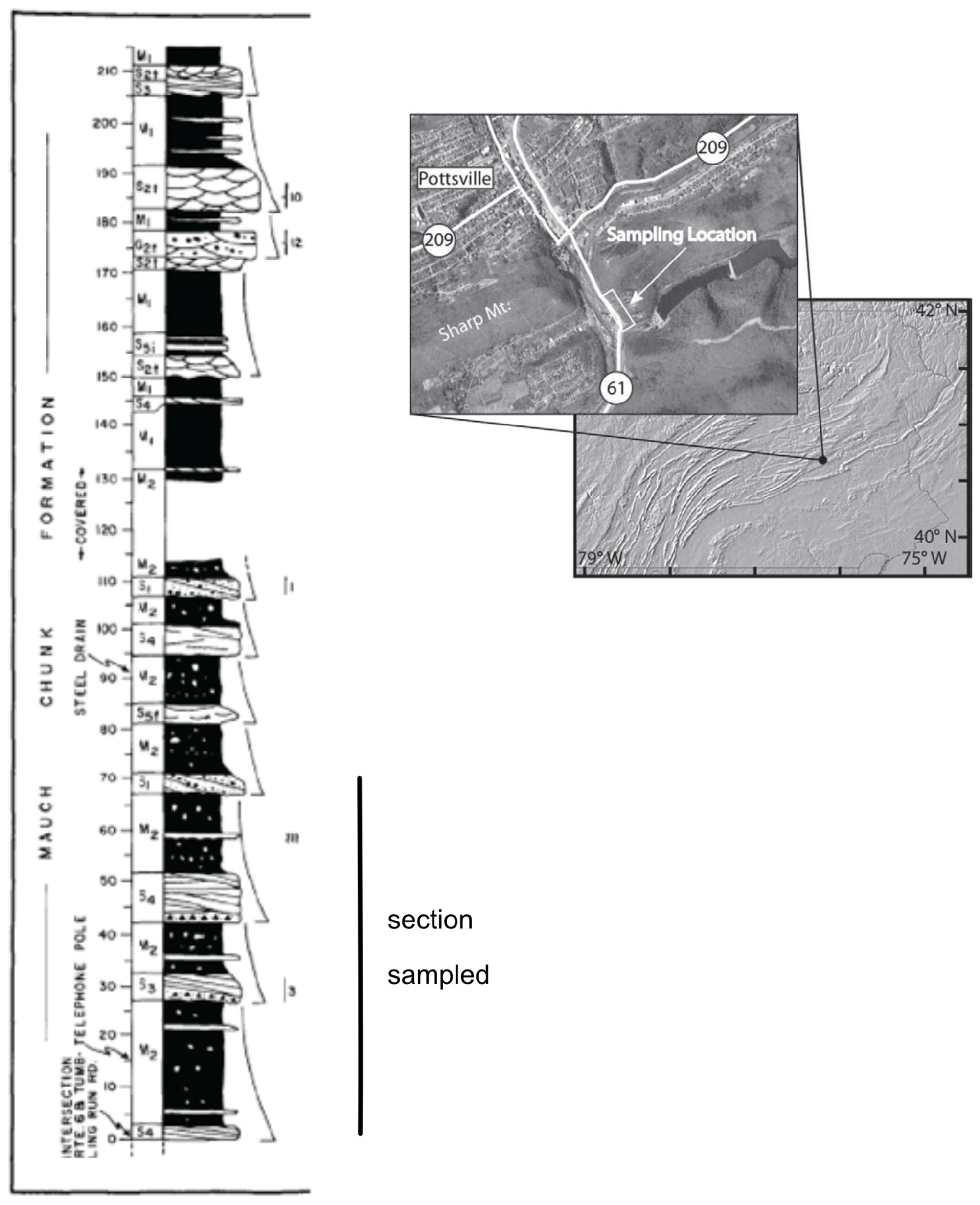
Figure 1. (Left) Stratigraphic column of the Pottsville, PA, Mauch Chunk Formation section from Levine and Slingerland (1987). (Right) Location of the Pottsville section of the Mauch Chunk Formation along Route 61 in northeastern Pennsylvania (from Bilardello and Kodama, 2010).

The Pottsville outcrop of the Mauch Chunk also offers a detailed magnetostratigraphy (DiVenere and Opdyke, 1991) which allows constraint of the sediment accumulation rate (SAR) thus allowing more robust identification of any Milankovitch cycles detected by the rock magnetics. The DiVenere and Opdyke (1991) magnetostratigraphy identifies a long (100 m thick) normal polarity event in the bottom part of the section where we have sampled. This normal event (MMCn at the Pottsville section) has been correlated to N5 in the Nova Scotia’s Maringouin Peninsula and the Joggins section and the MPN1 at the Broad Cove-Chapel section in Cape Breton Island by Opdyke et al. (2014) based primarily on biostratigraphy (palynology and fossil plants). This correlation suggests that 270.5 m of the Pottsville section represents 2.9 million years (Opdyke et al., 2014) yielding an average SAR of 9.3 cm/ka. The Geologic Time Scale 2012 (Gradstein et al., 2012) indicates that the MMCn normal polarity event is a little less than one million years in duration (SAR∼9–10 cm/ka) and is 330.9 Ma in age.

This paper will demonstrate that Milankovitch cycles (astronomically forced global climate change cycles of periodicities 100, 35, and ∼20 ka) can be detected rock magnetically in a fluvial depositional environment despite the presence of hiatuses in sedimentation typical of this environment. We will also show that measuring the susceptibility in the field with a portable susceptibility meter can yield a time series which records the same Milankovitch cycles.

Materials and Methods

To acquire the rock magnetic time series, we collected an un-oriented sample every 0.5 m of stratigraphic thickness, measuring stratigraphic thickness with a Jacob’s staff for the nearly vertically dipping strata at the Pottsville section. Based on the time series analysis theory, the shortest cycle detectable is the Nyquist frequency which is determined by the sample spacing.

$$\mathrm{Nyquist}\mathrm{frequency}=1/(2\times \mathrm{sample}\mathrm{spacing})$$

The shortest Milankovitch frequency we hoped to detect is precession which has periodicities of about 17.5 and 21 ka in the Carboniferous (Berger and Loutre, 1994; Waltham, 2015). Based on the SAR estimated from biostratigraphy and magnetostratigraphy (9.3 cm/ka), this would dictate sampling about every 80 cm of stratigraphic thickness to detect precession. Conservatively, we sampled every 50 cm.

In a pilot study, in 2012, a graduate level paleomagnetism class at Lehigh University sampled 40 m of the Pottsville section and measured isothermal remanent magnetization (IRMs) acquired in a 3.5 T field (IRM_3.5T). The measurements were normalized by sample mass. The magnetic susceptibility (χ) was also measured and the IRMs were alternating field demagnetized at 100 mT to remove the contributions of low coercivity ferromagnetic minerals to the IRM (IRM_3.5T–100mT).

In 2017, un-oriented samples were collected from 68 m of section, at a 0.5 m spacing. The rock samples were fitted into 2 × 2 × 2 cm³ plastic sample cubes and their magnetic susceptibility was measured in a KLY-3s Kappabridge. Each sample was measured three times and the measurements were averaged. The average measurements for each sample were normalized by sample mass. In the 2017 study, an SM-20 portable susceptibility meter was used to measure the bulk susceptibility at each place on the outcrop that the un-oriented samples were collected. The in situ susceptibility was measured at least three times on the flattest surface available and the results were averaged. The measurement is normalized by the volume that the SM-20 measures, approximately 49 cm³. The stratigraphic measurements were tied to the bottom of the Mauch Chunk Formation which outcrops at the Pottsville section.

Time series analysis was conducted using the multi-taper method (MTM, Thomson, 1982) with robust (Mann and Lees, 1996) red noise [Gilman et al., 1963; AR-1 autoregressive for both the portable (SM-20) and un-oriented rock samples (Kappabridge)]. Meyers’ (2014) and RStudio Team. (2015) was used for the analyses. Evolutionary spectrograms, using Astrochron, were also calculated to monitor how the dominant cycles varied throughout the section.

In the Astrochron time series analysis, outliers were trimmed from the time series using a box and whisker plot to reduce noise, the time series was resampled at an even spacing using linear interpolation, and MTM spectral analysis was conducted. In the MTM analysis 3 DPSS tapers were used, the mean was subtracted, the data were detrended and zero padded by a factor of 10. AR-1 robust red noise was calculated. Astrochron automatically identifies spectral peaks that are greater than a set value for the confidence level of the robust red noise and the harmonic f-test calculated by the MTM method (Meyers, 2012). The confidence levels were set at the default value (0.9) for the SM-20 time series and 0.85 for the Kappabridge time series.

To check our identification of the Milankovitch cycles, we conducted amplitude modulation (AM) analysis of the cycle we chose to be precession. The time series was filtered at the suspected precession frequency and time series analysis of the amplitude envelope of the filtered series was used to determine if there were cycles at the eccentricity time scale, because eccentricity modulates precession.

Low temperature (liquid N temperature, −195°C, warmed to 0°C) magnetic susceptibility versus temperature (MS vs. T) measurements were made in the KLY-3s Kappabridge to determine the proportion of paramagnetic (clays) and ferromagnetic (hematite and/or magnetite) minerals carrying the magnetic susceptibility. This was done following the constant ferromagnetic susceptibility method of Hrouda (1994) in which a hyperbola is fit to the magnetic susceptibility measured as the sample warmed from −195 to 0°C. The goodness of fit determines the percentage of paramagnetic minerals contributing to the bulk susceptibility. High temperature MS vs. T measurements in an argon atmosphere cycled up to 700°C and back down to room temperature were used to identify the ferromagnetic minerals.

Isothermal remanent magnetization acquisition experiments were also conducted to identify the ferromagnetic minerals in the samples. The IRM acquisition data were modeled using the Kruiver et al. (2001) Excel spreadsheet available from the Fort Hoofddijk paleomagnetic laboratory website.

All remanence measurements were conducted in a 2G Enterprises superconducting rock magnetometer (model 755) in a magnetically shielded room with a background magnetic field of ∼350 nT.

Results

Spectral Analysis

The time series constructed from IRM and MS measurements in the 2012 pilot study show a strong correlation between IRM_3.5T, IRM_3.5T–100mT and magnetic susceptibility, particularly at stratigraphic thickness wavelengths of 5–10 m, but also at shorter, 1–2 m scales (Figure 2 and Supplementary Table S2). The IRM_3.5T time series shows particularly high amplitude variation at the 1–2 m wavelength stratigraphic thickness scale. The big low in magnetic intensity for all three datasets at 25–30 m along the section correlates with a large sandstone bed indicating lithologic control of the susceptibility at this spatial scale. MTM spectral analysis using Astrochron of the IRM_3.5T–100mT time series shows significant spectral peaks at 6.8 m stratigraphic thickness (labeled 1) and 1.3 m stratigraphic thickness (labeled 2) (Figure 2). A third peak at ∼1.1 m stratigraphic thickness (labeled 3) is selected by Astrochron when the confidence level selection criterion is dropped to 0.85.

FIGURE 2

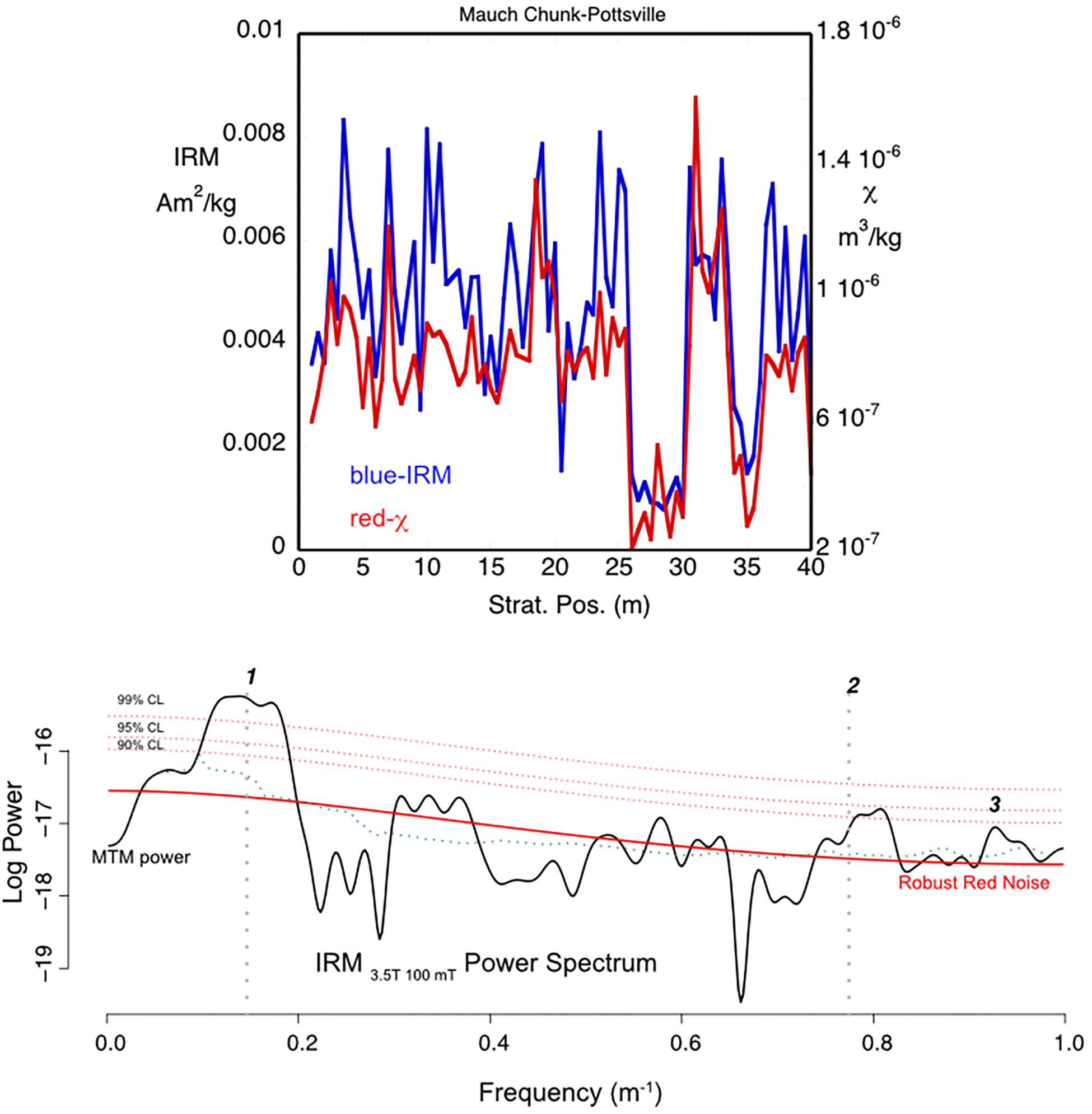
Figure 2. (Top) Time series of IRM acquired in a 3.5 T field and then alternating field demagnetized at 100 mT (blue curve) and magnetic susceptibility (red curve) for the 40 m of Pottsville section measured in 2012 by the graduate class at Lehigh University. Both curves show both long period and short period oscillations in phase with each other. The amplitudes of the variation are greater for the IRM. (Bottom) The MTM (Thomson, 1982) power spectrum for the IRM calculated by Astrochron indicates two significant peaks, one at 6.8 m stratigraphic thickness (labeled 1) and 1.3 m stratigraphic thickness (labeled 2). A third significant peak (∼1.1 m-labeled 3) is selected by Astrochron when the confidence level selection criterion is dropped from 0.9 to 0.85.

For the 2017 dataset, the main study of this paper, the magnetic susceptibility time series for the Kappabridge, laboratory rock sample measurements and the SM-20 portable susceptibility meter measurements both show high amplitude, high frequency (∼1 m stratigraphic thickness periods) content (Figure 3 and Supplementary Table S1). The Kappabridge time series shows a better correlation with the lithologic column with longer wavelength lows associated with sandstone beds. Both time series show high amplitude, high frequency variability within the mudstone overbank deposits exposed between 5 m and about 28 m in the section, indicating that the magnetic susceptibility isn’t controlled completely by lithologic variations. Both time series show hierarchical frequency variability, as would be expected for records of different Milankovitch cycles, but the two different time series (SM-20 and Kappabridge) cannot be easily correlated.

FIGURE 3

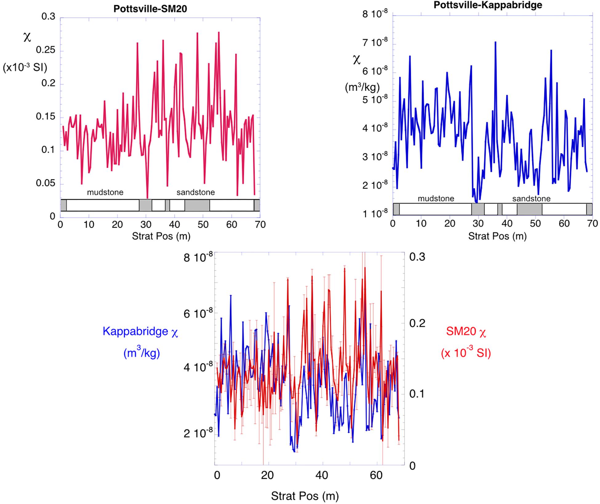
Figure 3. Time series magnetic susceptibility for 68 m of the Pottsville section measured by the SM-20 portable susceptibility meter (Top left) and for rock samples collected in the field and measured on the Kappabridge KLY-3s at the Lehigh University (Top right). Below each plot is the stratigraphy for the 68 m samples showing the sandstone channel deposits and the mudstone overbank deposits. Base of the section is to the left. Both time series show both long period and short period variability; however, they do not match. The Kappabridge measured susceptibility shows better correlation to the lithologic variations at long periods, but both time series show short period variations within the different lithologies. A direct comparison of the two time series (Bottom center), with one standard deviation error bars, shows the high uncertainty in the SM-20 measurements compared to the low uncertainty in the Kappabridge measurements (error bars are typically smaller than the symbol for the measurement).

A direct comparison of the two time series, including errors bars (one standard deviation), shows that the SM-20 portable susceptibility meter dataset has much higher uncertainty in its measurements. The uncertainty in the SM-20 measurements could be the explanation for the differences in the two time series (Figure 3). Given this obvious difference in the two time series, collected by different types of measurement, it is interesting that for the MTM spectral analyses, Astrochron (Meyers, 2014) picks very similar significant peaks using both robust red noise (Mann and Lees, 1996) and harmonic f-test (Thomson, 1982) as selection criteria, for both series (Figures 4, 5 and Tables 1, 2).

FIGURE 4

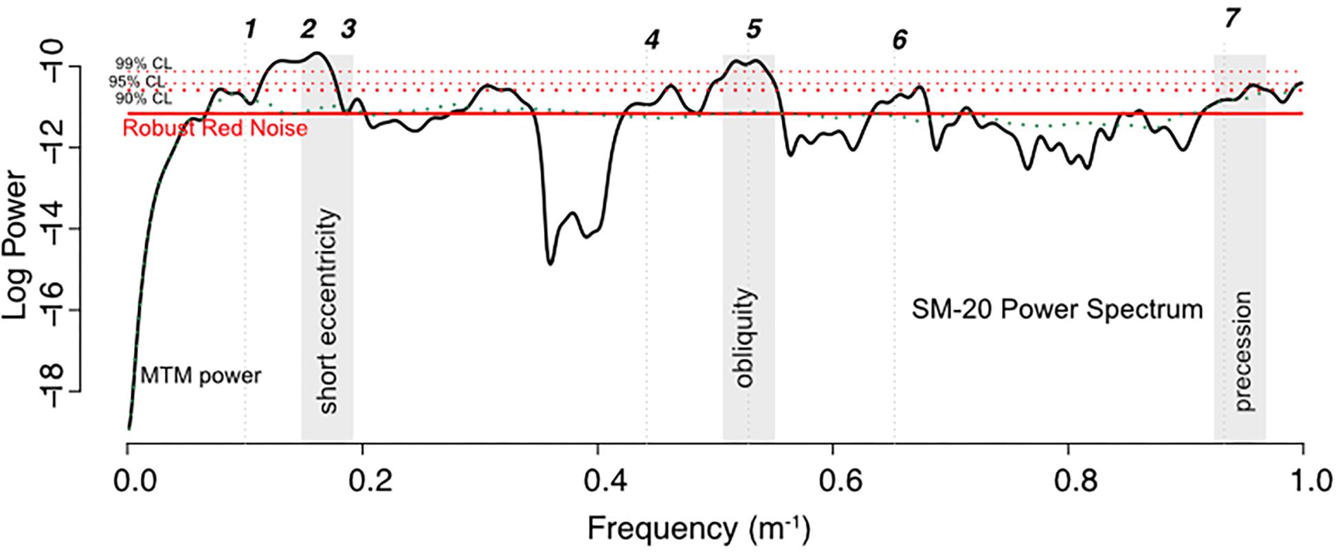
Figure 4. Log power spectrum for the SM-20 portable susceptibility meter magnetic susceptibility time series shown in Figure 3 showing significant peaks chosen by Astrochron (Meyers, 2014) and numbered (confidence limit set to 0.9). The shaded bands show our choice for the Milankovitch cycles. See Table 1 for the periods/frequencies of the numbered peaks.

FIGURE 5

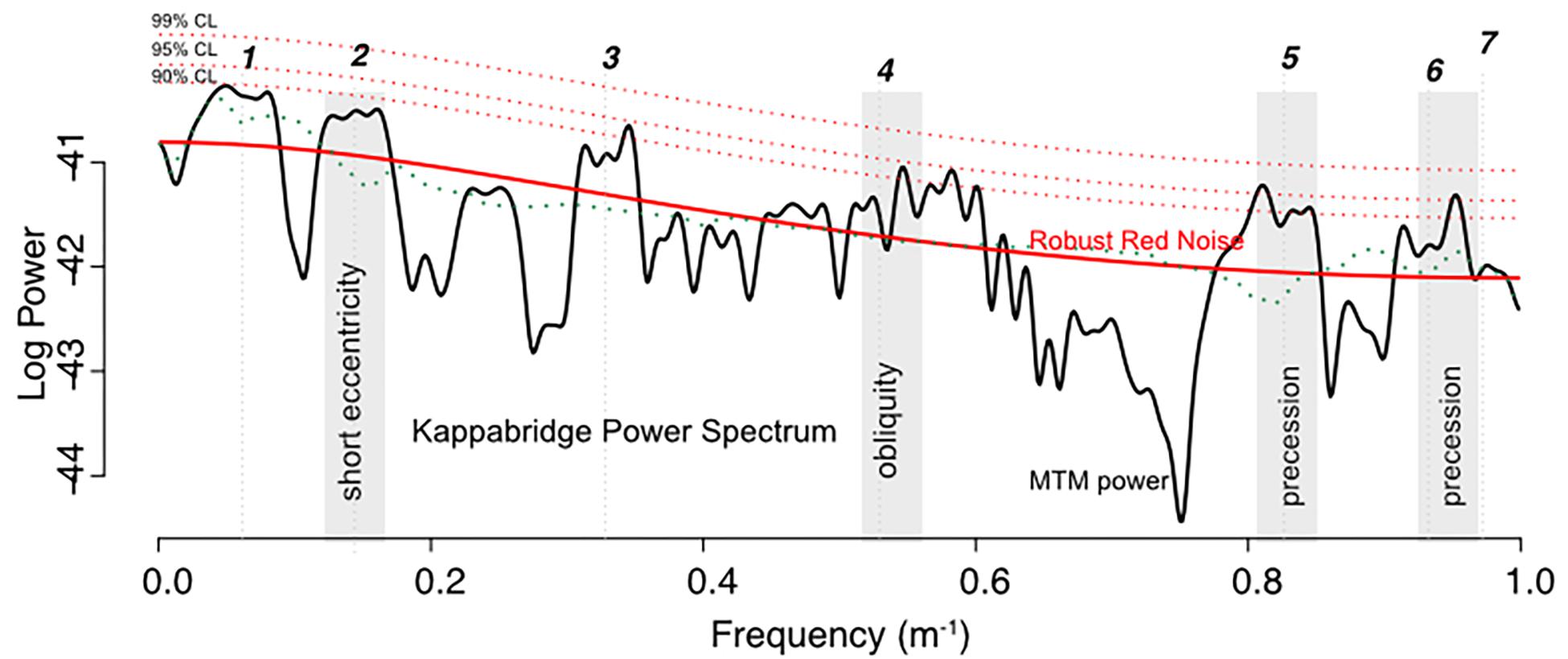
Figure 5. Log power spectrum for the Kappabridge measured magnetic susceptibility time series shown in Figure 3 showing significant peaks chosen by Astrochron (Meyers, 2014) and numbered (confidence limit set to 0.85). The shaded bands show our choice for the Milankovitch cycles. See Table 2 for the periods/frequencies of the numbered peaks.

TABLE 1

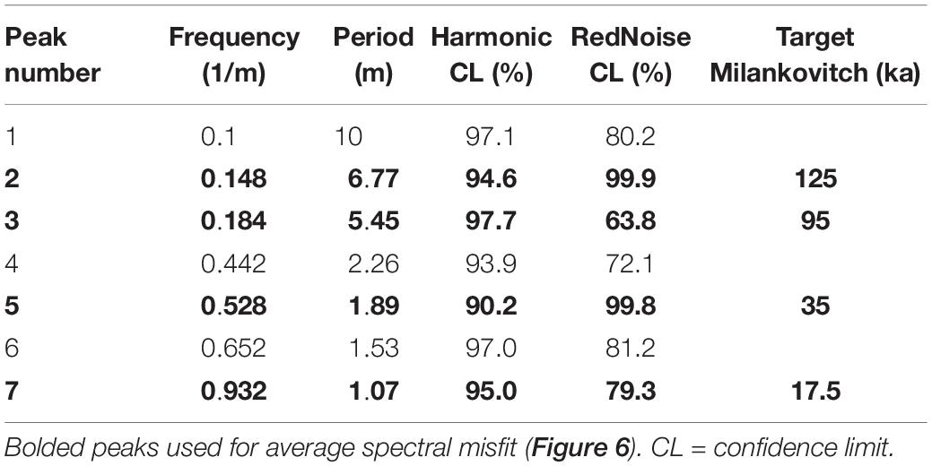
Table 1. Portable SM-20 spectral peaks.

TABLE 2

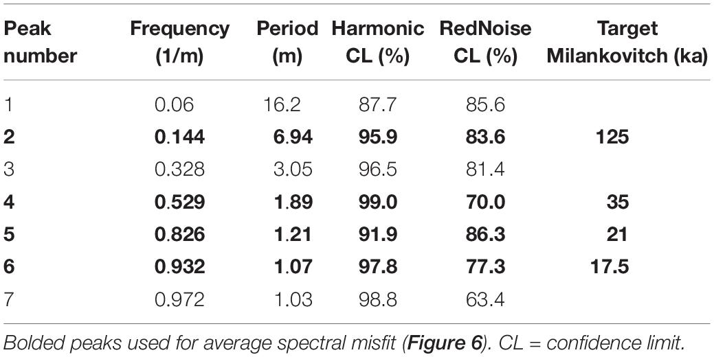
Table 2. Laboratory sample – Kappabridge spectral peaks.

The most striking similarities between the two time series are spectral peaks at 6.8, 1.9, and 1.1 m. The ratio of these peaks is similar to the ratios of short eccentricity (125 ka), obliquity (35 ka), and short precession (17.5 ka) at 330 Ma (Waltham, 2015). Thus, we have tentatively identified these peaks as the short eccentricity, obliquity and precession Milankovitch cycles in the Carboniferous. Note that the 5.45 m peak in the SM-20 data (Table 1) could be 95 ka short eccentricity, and the 1.21 m peak in the Kappabridge data (Table 2) could be long precession (21 ka). Note also that the peaks identified from the longer 68 m section are very similar to those observed for the IRM_3.5T–100mT measured for the 40 m pilot study. The IRM times series peak at 6.8 m is identified as short eccentricity, the 1.3 and 1.1 m peaks are long and short precession.

We can test these picks using average spectral misfit (ASM) in the Astrochron software package (Meyers and Sageman, 2007; Meyers, 2014). It iteratively tries different SARs to fit the selected spectral peak frequencies to Milankovitch target frequencies. It tests the significance level of the null hypothesis for the best fit SAR (Meyers, 2014). ASM gives statistically significant fits, at greater than 98%, for both the SM-20 series and the Kappabridge time series yielding the identical SAR of 5.69 cm/ka for both time series (Figure 6).

FIGURE 6

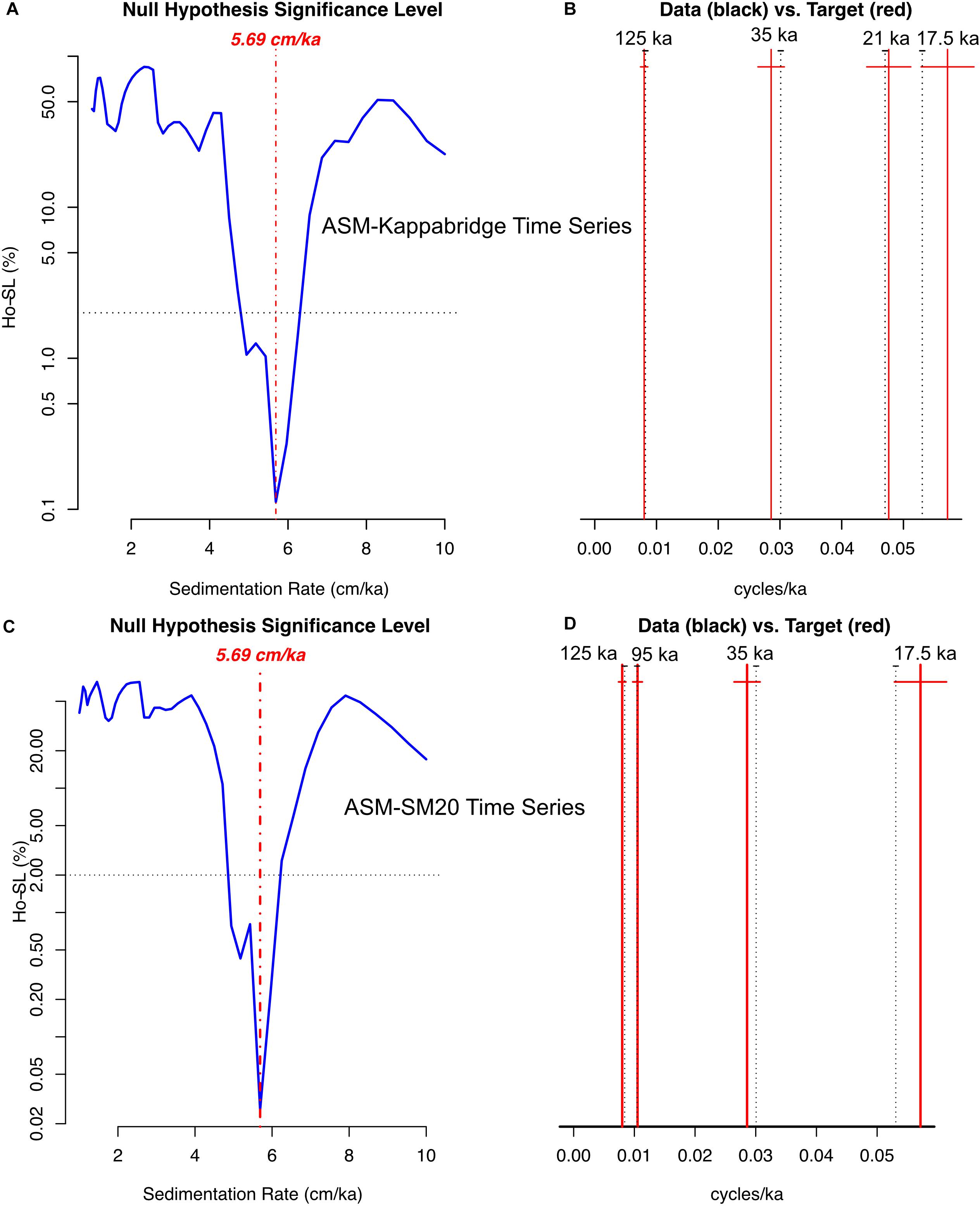
Figure 6. Average spectral misfit (ASM; Meyers and Sageman, 2007) results for the Kappabridge (A) and SM-20 (B) spectral peaks targeted to eccentricity, obliquity, and precession at 330 Ma. The significant fit for the two different time series indicates an identical sediment accumulation rate of 5.69 cm/ka. In panels (C) and (D), the dotted black lines are the data and the red solid lines are the target Milankovitch frequencies.

Finally, we can test our Milankovitch picks by conducting an AM test of the precession (17.5 ka) cycle we have identified in our spectral analysis. Precession should be modulated by eccentricity, so if we picked precession correctly its amplitude should be modulated by the frequency we have selected as eccentricity. Astrochon (Meyers, 2014) provides a testPrecession routine that could accomplish this test, however, an accurate theoretical model of precession is needed. This exists only as far back in time as the Paleogene, therefore, we conducted our own version of this test. We filtered the Kappabridge rock sample time series at 0.93 m^–1 (the 1.07 m spectral peak) and the resulting filtered series showed AM with six peaks per pulse (Figure 7). We conducted MTM spectral analysis on the amplitude envelope of the filtered series and found a strong peak with a frequency of 0.14 m^–1, which is exactly the 125 ka eccentricity peak we targeted with our ASM analysis. The AM test shows that we have correctly selected precession and eccentricity in our spectral analysis.

FIGURE 7

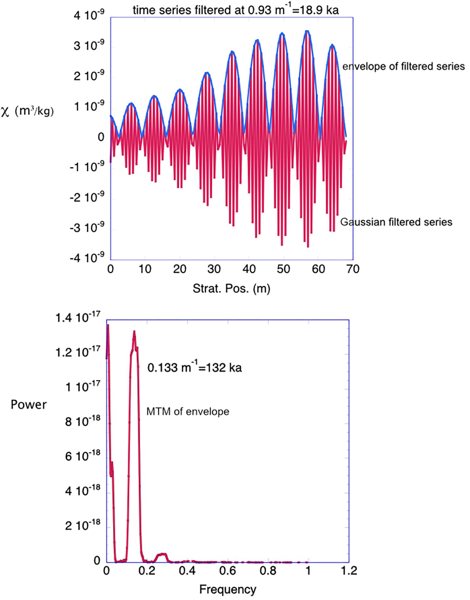
Figure 7. Amplitude modulation (AM) test conducted on the frequency chosen for precession in our results. (Top) The Kappabridge time series was filtered at the frequency of the spectral peak chosen to be precession (0.93 m^–1) and the envelope of the amplitude variation yields a power spectrum (Bottom) with a significant peak at the frequency we have chosen as short eccentricity (0.133 m^–1). This result strongly supports our assignment of Milankovitch frequencies to the spectral peaks observed in our data.

Evolutionary spectrograms of the portable (SM-20) and laboratory-measured rock samples (Kappabridge) time series (Figure 8) show that for the portable susceptibility meter data all three of the Milankovitch cycles are stronger in the upper part of the section, starting at about 30 m for the short eccentricity and obliquity, but only at about 40 m for the precession cycle. For the Kappabridge-measured rock samples (Figure 8) the eccentricity cycles (both long and short eccentricity, 405 and 100 ka) are strong throughout the section while obliquity and precession [both long (21 ka) and short (17.5 ka)] vary in strength throughout the section. The most important observation is that the SAR doesn’t appear to change throughout the section. The evolutionary spectrograms are compared to the MTM power spectra for each time series. These spectra were calculated by the SSA-MTM toolkit (Ghil, 1997) with robust red noise (Mann and Lees, 1996) and are identical to the power spectra calculated from Astrochron (Figure 5); however, using Astrochron’s selection criteria (robust red noise and harmonic f-test) the peak labeled long eccentricity (le) has a wavelength of only 10 m, which would only be 175.7 ka for the 5.69 cm/ka SAR calculated by ASM and would not be consistent with long eccentricity, 405 ka. However, the maximum amplitude of the le peak yields a wavelength of 22.5 m, indicating a period of 395.4 ka for an SAR of 5.69 cm/ka, entirely consistent with long eccentricity. Therefore, the Kappabridge time series also contains a record of long eccentricity which repeats approximately three times in our record. The 40 m IRM time series collected in 2012 is too short to observe long eccentricity.

FIGURE 8

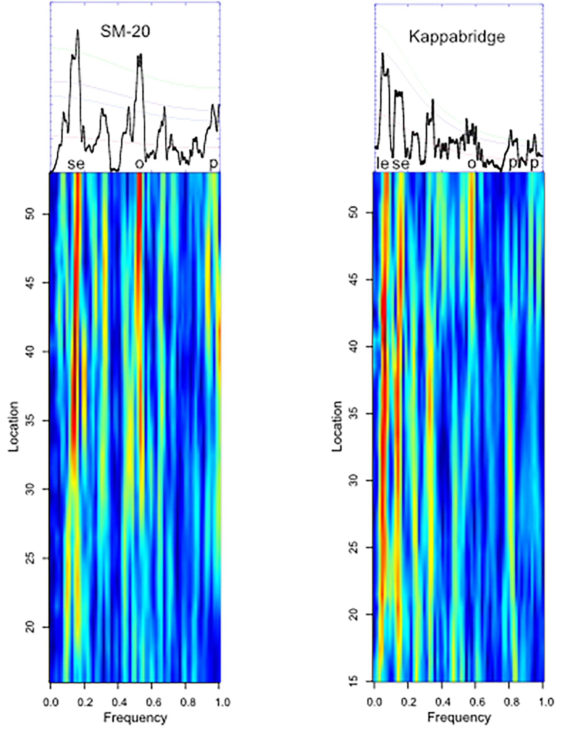
Figure 8. Evolutionary spectrograms calculated using Astrochron (Meyers, 2014) for the SM-20 (Left) and the Kappabridge measured samples (Right). The MTM calculated power spectrum for each series (using SSA-MTM) is shown at the top of each evolutionary spectrogram with Milankovitch spectral peaks labeled (le = long eccentricity, se = short eccentricity, o = obliquity, p = precession). The evolutionary spectrograms were calculated with a window of 30 m and a step of 1 m. They show that the sediment accumulation rate does not vary significantly through the section although the power of the different frequencies does vary.

Rock Magnetics

The MS vs. T plots measured at temperatures between 20 and 700°C indicate the weak occurrence of magnetite but mainly the presence of hematite in the Mauch Chunk Formation samples (Figure 9). On cooling from high temperatures the strong increase in susceptibility at 580°C indicates that magnetite has been created by the heating. This behavior is observed for both a mudstone and a sandstone sample. The low temperature MS vs. T plots measured at temperatures between −195 and 0°C show no evidence of a Verwey transition, so magnetite is not present in any great abundance (Figure 9). These results are supported by the IRM acquisition experiments (Figure 10) which show that the IRM for the Mauch Chunk Formation samples saturates at about 3 T. Modeling of the IRM acquisition data shows that most (97%) of the IRM acquisition data could be fit with a coercivity component of about 0.5–0.6 T indicating a high coercivity mineral, most likely hematite. A very small component (∼3% of the IRM) could be fit with a low coercivity (65 mT) mineral, probably a small amount of magnetite.

FIGURE 9

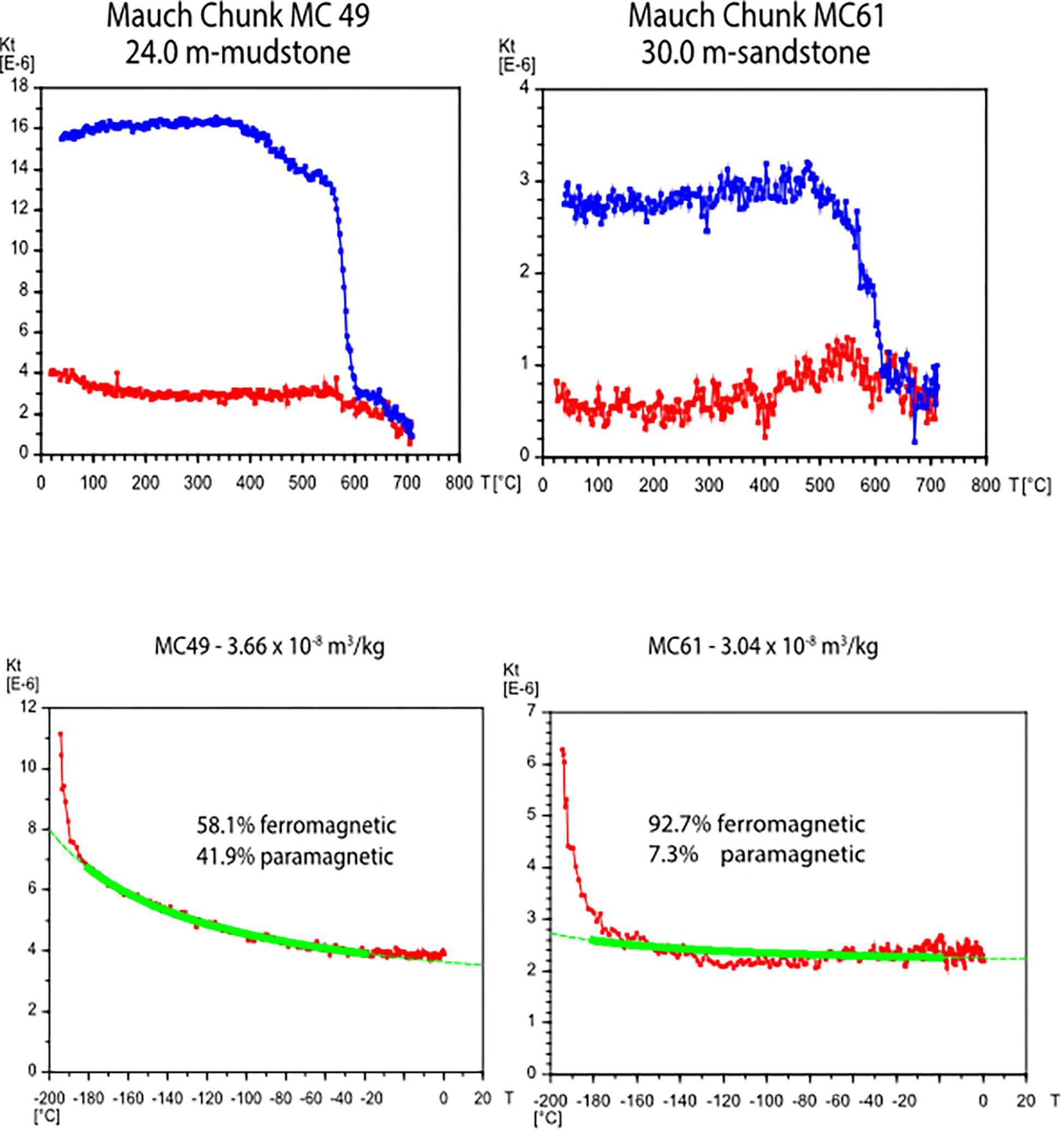
Figure 9. High and low temperature MS vs. T results measured on the Kappabridge for a sample representative of a mudstone lithology and a sandstone lithology. The low temperature results are fit by a paramagnetic hyperbola to determine the relative proportion of ferromagnetic and paramagnetic contributing to the magnetic susceptibility (Hrouda, 1994).

FIGURE 10

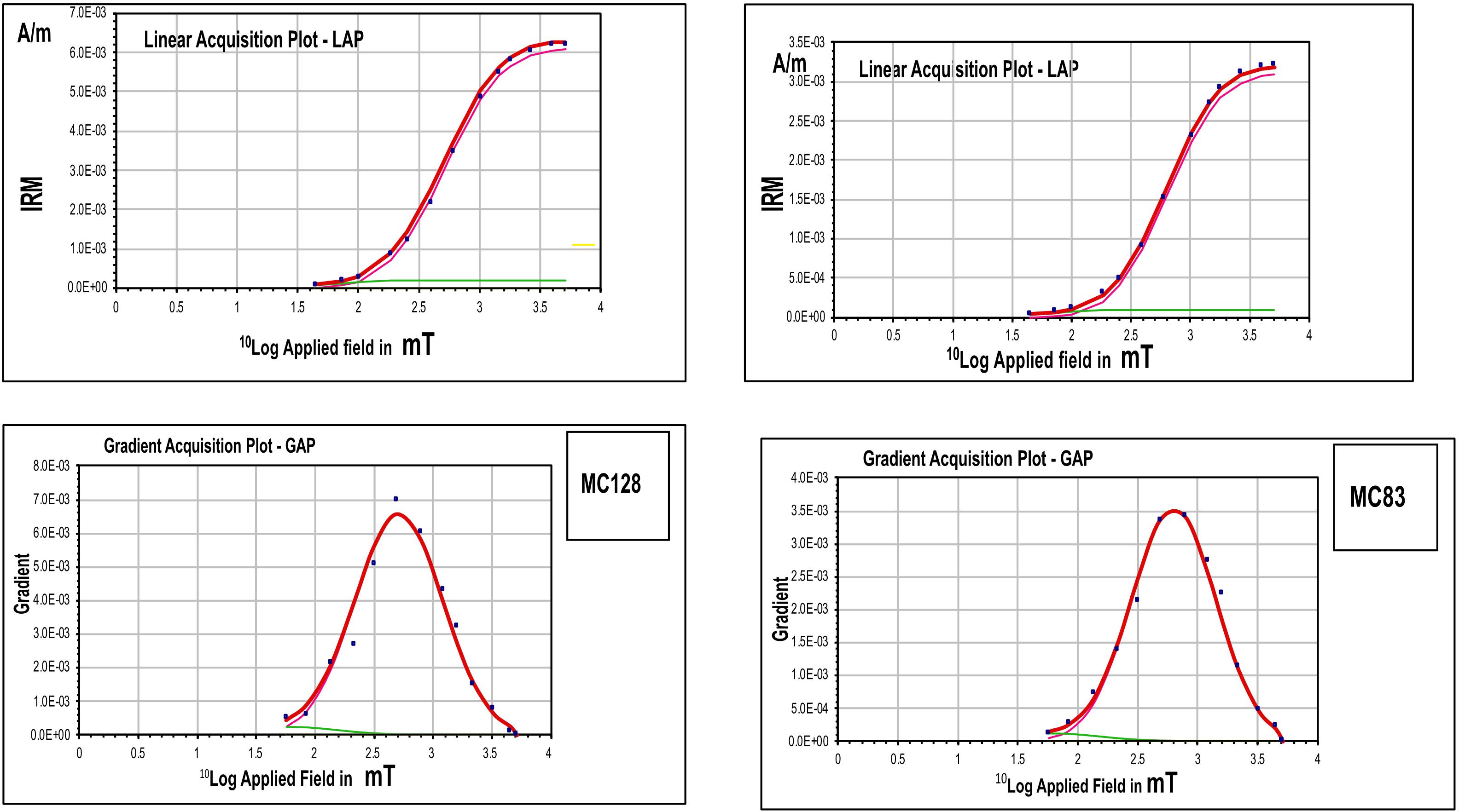
Figure 10. Isothermal remanent magnetization acquisition results showing that the samples are dominated by a high coercivity remanence that saturates by 3.5 T and is probably hematite. There is a minor contribution from a lower coercivity component that is probably magnetite.

The relative proportion of ferromagnetic (hematite) and paramagnetic (clay) contributing to the bulk susceptibility was estimated for 21 samples over a 10 m stratigraphic interval between 20.5 and 30.5 m in the section. The stratigraphic interval included both the red mudstone overbank deposits and the sandstone channel deposits. An example of the hyperbola fit to the low temperature measurements for a mudstone and a sandstone sample to estimate paramagnetic/ferromagnetic content is shown in Figure 9. The contribution of paramagnetic and ferromagnetic to the total susceptibility was determined by multiplying the percentage of each by the bulk susceptibility for a sample (Figure 11). Two repeated measurements for both a mudstone and a sandstone sample show the percentage estimates are repeatable within about 7% points. The high frequency peaks in bulk susceptibility with a wavelength of 1–2 m are driven mainly by variations in the ferromagnetic minerals. The ferromagnetic minerals are the only contributor to the bulk susceptibility in the sandstone (Figure 11). The paramagnetic minerals also drive some of the peaks in the bulk susceptibility. They are sometimes in phase with the ferromagnetic mineral variations and sometimes out of phase. In the 10 m stratigraphic interval measured for this analysis, there are six ferromagnetic peaks which match the six peaks in the bulk susceptibility, suggesting a wavelength of ∼1.5 m, whereas the paramagnetic minerals show two large peaks in phase with the ferromagnetic peaks and possibly an additional two smaller peaks that do not coincide with peaks in the bulk susceptibility. When these estimates of stratigraphic wavelength are compared to the spectral analysis of the Kappabridge time series (Table 2), it strongly suggests that ferromagnetic mineral concentration variations are a strong control on the bulk MS variations that record astronomically forced climate change (Milankovitch) cycles at precession (20 ka) and obliquity (35 ka) frequencies. Given the 10 m length of the stratigraphic interval used for this analysis, it is not possible to determine if ferromagnetic or paramagnetic minerals are beating at the eccentricity period of ∼7 m.

FIGURE 11

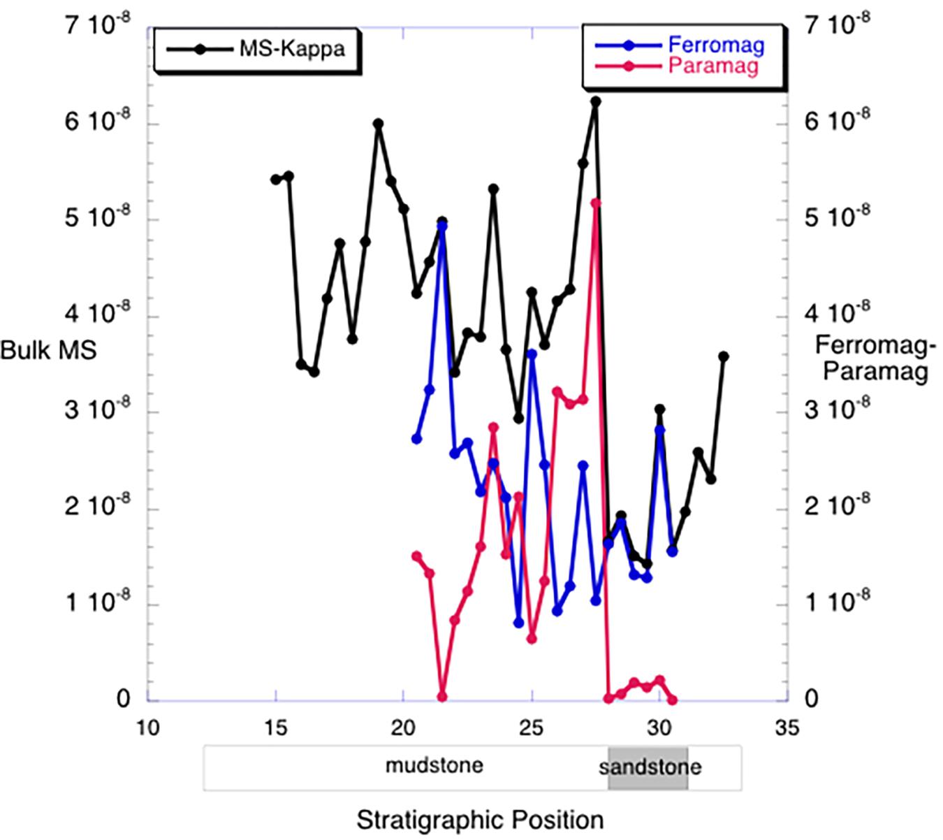
Figure 11. The relative proportion of ferromagnetic minerals (blue curve) and paramagnetic minerals (red curve) contributing to the bulk susceptibility (black curve) for 10 m between 20.5 and 30.5 m in the section. The percentages determined from the low temperature MS vs. T measurements have been multiplied by the bulk susceptibility for a sample to determine the susceptibility for each magnetic mineral type. Note that the blue (ferromagnetic) curve follows all the short period peaks in the bulk susceptibility curve (black curve) indicating that the ferromagnetic mineral variations are the source of the bulk susceptibility variations. The paramagnetic mineral contribution is sometimes in phase with the ferromagnetic variations, sometimes out of phase. The magnetic susceptibility of the sandstone bed is almost all due to ferromagnetic minerals.

Discussion

Recording Milankovitch Cycles

The MS time series collected with the SM-20 portable susceptibility meter and the Kappabridge measurement of rock samples both showed a record of Milankovitch cycles at periods of 100, 35, and 20 ka and the IRM time series showed Milankovitch cycles at 100 and 20 ka. ASM analysis (Meyers, 2014) of both the portable and Kappabridge MS time series indicate a SAR of 5.69 cm/ka showing that the 5–7 m wavelength peaks are short eccentricity at 125 and 95 ka, the 1.9 m peak is obliquity at 35 ka, and the 1.2–1.1 m wavelength peaks are precession at 21 and 17.5 ka. AM analysis shows that the 1.07 m wavelength peak, picked to be short precession at 17.5 ka, is modulated by a frequency of about 0.14 cycles/m which is our pick for short eccentricity at 125 ka. This result supports our pick for Milankovitch cycles in the data.

Our results indicate that a fluvial, terrigenous depositional environment can record Milankovitch global climate cycles despite the expectation that this type of environment will experience discontinuous sedimentation (i.e., flooding into the overbank environment) and the effects of environmental shredding (Jerolmack and Paola, 2010) due to landscape processes, such as avulsion (channel migration). Our results would suggest, in light of Jerolmack and Paola’s analysis, that the shortest Milankovitch cycle recorded (i.e., precession at 17.5 ka) is still a longer period than shredding processes in the depositional basin (e.g., flooding and avulsion).

The SAR derived from these high resolution chronostratigraphy results suggests that the long normal polarity interval of the Earth’s geomagnetic field recorded at the Pottsville section and correlated throughout eastern North America (Opdyke et al., 2014) is 1.75 million years in duration and not 1.0 million years as suggested by biostratigraphy (Opdyke et al., 2014) and may help more accurately calibrate this part of the geologic time scale in the Carboniferous (Gradstein et al., 2012).

Encoding the Milankovitch Signal

The strong positive correlation between the percentage of ferromagnetic minerals contributing to the magnetic susceptibility and the bulk susceptibility variations suggests erosion in the source area, driven by climate change, is adding more or less depositional hematite to a background of either clay minerals or quartz sand in the depositional basin at the Milankovitch time scales. Therefore, changes in the source area for the Mauch Chunk sediments are encoding the Milankovitch cycles rather than changes in the depositional basin. This is similar to the record of Milankovitch cycles in marine sediments in which variations in precipitation on the continent changes the supply of clastic sediments into a background of carbonate production in the near-shore marine environment (Kodama et al., 2010; Gong et al., 2017; Minguez and Kodama, 2017). The record of eccentricity and precession by the Mauch Chunk Formation sediments is consistent with its 23°S paleolatitude (Bilardello and Kodama, 2010) where the strength of the monsoon is driven by eccentricity and precession. However, it is interesting that rock magnetics also detect obliquity for this low paleolatitude because obliquity insolation variations are stronger at high latitudes than low latitudes. In support of our results, Gunderson et al. (2012) did observe a strong obliquity signal in Mediterranean (low latitude) Plio-Pleistocene sediments recorded by magnetic susceptibility. The weak coupling of paramagnetic minerals to the shorter Milankovitch frequencies could be due to variations in chemical weathering in the source area being driven by global climate change.

Portable Susceptibility Meter Measurements

Even though the portable susceptibility meter measurements did not observe exactly the same time series as the more accurate Kappabridge measurements of rock samples, and could not be normalized by sample mass, the spectral analysis of the portable time series was still able to detect the same Milankovitch cycles as the Kappabridge-rock sample measurements. This result indicates that using the portable susceptibility meter for rock magnetic cyclostratigraphy is a valid method for constructing a time series, particularly for clastic, relatively high magnetic mineral content, sedimentary rocks. Conceivably, the portable susceptibility measurements could be used for reconnaissance work to accurately set the sampling interval for more detailed sample collection and rock magnetic measurements in the laboratory.

Conclusion

Both measurements in the field using a portable susceptibility meter and magnetic susceptibility and IRM measurement of rock samples in the laboratory could detect Milankovitch cycles in a fluvial depositional environment recorded by depositional hematite grains in red beds deposited during the Carboniferous. This is an important result because it opens up terrestrial, fluvial deposits to the high-resolution dating and correlation afforded by rock magnetic cyclostratigraphy.

A SAR of 5.69 cm/ka derived from both the portable susceptibility meter and the rock sample measurements suggests that the long normal polarity interval in the Pottsville Mauch Chunk Formation section is 1.75 million years in duration, not <1 million years as previously indicated by the biostratigraphy and suggests a slight recalibration of this part of the Carboniferous geologic time scale is needed.

The astronomically forced, Milankovitch-scale climate cycles were probably encoded by variations in erosion of the source area supplying varying amounts of depositional hematite into a background of paramagnetic clay minerals or diamagnetic quartz sand in the depositional basin.

Data Availability Statement

The raw data supporting the conclusion of this manuscript will be made available by the author, without due reservation, to any qualified researcher. The susceptibility measurements are available in the Supplementary Material.

Author Contributions

KK made susceptibility measurements, helped to collect the samples, analyzed the data, and wrote the manuscript.

Funding

This study was partially supported by NSF-EAR 1322002.

Conflict of Interest

The author declares that the research was conducted in the absence of any commercial or financial relationships that could be construed as a potential conflict of interest.

Acknowledgments

Marta Sanchez Anson collected the 68 m section, measured in situ susceptibilities with the portable susceptibility meter, prepared the laboratory samples for measurement, and made some of the Kappabridge measurements. Daniel Minguez and Nathan Hopkins collected the 2012 samples for the pilot study and made the laboratory measurements of IRM and susceptibility.

Supplementary Material

The Supplementary Material for this article can be found online at: https://www.frontiersin.org/articles/10.3389/feart.2019.00285/full#supplementary-material

TABLE S1 | Laboratory Kappabridge and portable SM-20 susceptibility measurements for the Pottstown section of the Mauch Chunk Formation.

TABLE S2 | IRM (3.5 T), IRM (3.5 T demagnetized at 100 mT), and magnetic susceptibility measurements (kappabridge) for the 2012 study of the Mauch Chunk Formation at the Pottsville section.

References

Abdul Aziz, H., Hilgen, F., Krijgsman, W., Sanz, E., and Calvo, J. P. (2000). Astronomical forcing of sedimentary cycles in the middle to late miocene continental Calatayud Basin (NE Spain). Earth Planet. Sci. Lett. 177, 9–22. doi: 10.1016/s0012-821x(00)00035-2

CrossRef Full Text | Google Scholar

Abels, H. A., Kraus, M. J., and Gingerich, P. D. (2013). Precession-scale cyclicity in the lower eocene fluvial willwood formation of the bighorn basin. Wyoming (USA). Sedimentology 60, 1467–1483.

Google Scholar

Berger, A., and Loutre, M. F. (1994). Astronomical forcing through geological time. Spec. Publs. Int. Assoc. Sediment 19, 15–24. doi: 10.1002/9781444304039.ch2

CrossRef Full Text | Google Scholar

Bilardello, D. A., and Kodama, K. P. (2010). A new inclination shallowing correction of the mauch chunk formation of pennsylvania, based on high-field AIR results: implications for the carboniferous north american APW path and pangea reconstructions. Earth Planet. Sci. Lett. 299, 218–227. doi: 10.1016/j.epsl.2010.09.002

CrossRef Full Text | Google Scholar

Cioppa, M. T., and Kodama, K. P. (2003). Evaluation of paleomagnetic and finite strain relationships due to the alleghanian orogeny in the mississippian mauch chunk formation, pennsylvania. J. Geophys. Res. 108, 1–16.

Google Scholar

DiVenere, V. J., and Opdyke, N. D. (1991). Magnetic polarity stratigraphy in the uppermost mississippian mauch chunk formation pottsville, pennsylvania. Geology 19, 127–130.

Google Scholar

Ghil, M. (1997). “The SSA-MTM toolkit: applications to analysis and prediction of time series,” in Proceedings of Optical Science, Engineering and Instrumentation, San Diego, CA.

Google Scholar

Gilman, D., Fuglister, R., and Mitchell, J. Jr. (1963). On the power spectrum of “red noise”. J. Atmos. Sci. 20, 182–184. doi: 10.1175/1520-0469(1963)020<0182:otpson>2.0.co;2

CrossRef Full Text | Google Scholar

Gong, Z., Kodama, K. P., and Li, Y.-X. (2017). Rock magnetic cyclostratigraphy of the doushantuo formation. Precambrian Res. 289, 62–74.

Google Scholar

Gradstein, F. M., Ogg, J. G., Schmitz, M. D., and Ogg, G. M. (eds) (2012). The Geologic Time Scale 2012 (Oxford: Elsevier), 1144.

Google Scholar

Gunderson, K. L., Kodama, K. P., Anastasio, D. J., and Pazzaglia, F. J. (2012). Rock magnetic cyclostratigraphy for the late pliocene-early pleistocene stirone section. Geol. Soc. Lond. Spec. Publ. 373, 309–323. doi: 10.1144/SP373.8

CrossRef Full Text | Google Scholar

Hinnov, L. A. (2013). Cyclostratigraphy and its revolutionizing applications in the earth and planetary sciences. Geol. Soc. Am. Bull. 125, 1703–1734. doi: 10.1130/B30934.1

CrossRef Full Text | Google Scholar

Hrouda, F. (1994). A technique for the measurement of thermal changes of magnetic susceptibility of weakly magnetic rocks by the CS-2 apparatus and KLY-2 Kappabridge. Geophys. J. Int. 118, 604–612. doi: 10.1111/j.1365-246x.1994.tb03987.x

CrossRef Full Text | Google Scholar

Jerolmack, D. J., and Paola, C. (2010). Shredding of environmental signals by sediment transport. Geophys. Res. Lett. 37:L19401.

Google Scholar

Kent, D. V., and Opdyke, N. D. (1985). Multicomponent magnetizations from the mississippian mauch chunk formation of the central appalachians and their tectonic implications. J. Geophys. Res. 90, 5371–5383. doi: 10.1029/jb090ib07p05371

CrossRef Full Text | Google Scholar

Kodama, K. P., Anastasio, D. J., Newton, M. L., Pares, J., and Hinnov, L. A. (2010). High resolution rock magnetic cyclostratigraphy in an eocene flysch, spanish pyrenees. Geochem. Geophys. Geosys. 11:Q0AA07. doi: 10.1029/2010GC003069

CrossRef Full Text | Google Scholar

Kodama, K. P., and Hinnov, L. A. (2015). Rock Magnetic Cyclostratigraphy. Blackwell: Wiley, 165.

Google Scholar

Kruiver, P. P., Dekkers, M. J., and Heslop, D. (2001). Quantification of magnetic coercivity components by the analysis of acquisition curves of isothermal remanent magnetization. Earth Planet. Sci. Lett. 189, 269–276. doi: 10.1016/s0012-821x(01)00367-3

CrossRef Full Text | Google Scholar

Levine, J. R., and Slingerland, R. (1987). Upper mississippian to middle pennsylvanian stratigraphic section. Geol. Soc. Am. Centen. 15, 59–63.

Google Scholar

Mann, M., and Lees, J. (1996). Robust estimation of background noise and signal detection in climatic time series. Clim. Chang. 33, 409–445. doi: 10.1007/BF00142586

CrossRef Full Text | Google Scholar

Meyers, S. R. (2012). Seeing red in cyclic stratigraphy: spectral noise estimation for astrochronology. Paleoceanogr. Paleoclimatol. 27:PA3228. doi: 10.1029/2012PA002307

CrossRef Full Text | Google Scholar

Meyers, S. R. (2014). Astrochron: an R Package for Astrochronology. Available at http://cran.r-project.org/package=astrochron

Google Scholar

Meyers, S. R., and Sageman, B. B. (2007). Quantification of deep-time orbital forcing by average spectral misfit. Am. J. Sci. 307, 773–792. doi: 10.2475/05.2007.01

CrossRef Full Text | Google Scholar

Minguez, D., and Kodama, K. P. (2017). Rock magnetic chronostratigraphy of the shuram carbon isotope excursion: wonoka formation. Aust. Geol. 45, 567–570. doi: 10.1130/g38572.1

CrossRef Full Text | Google Scholar

Minguez, D., Kodama, K. P., and Hillhouse, J. W. (2015). Paleomagnetic and cyclostratigraphic constraints on the synchroneity and duration of the shuram carbon isotope excursion, johnnie formation, death valley region, CA. Precambrian Res. 266, 395–408. doi: 10.1016/j.precamres.2015.05.033

CrossRef Full Text | Google Scholar

Noorbergen, L. J., Abels, H. A., Hilgen, F. J., Robson, B. E., Jong, E. D., Dekkers, M. J., et al. (2018). Conceptual models for short-eccentricity climate control on peat formation in a lower Palaeocene fluvial system, northeaster montana (USA). Sedimentology 65, 775–808. doi: 10.1111/sed.12405

CrossRef Full Text | Google Scholar

Opdyke, N. D., Giles, P. S., and Utting, J. (2014). Magnetic polarity stratigraphy and palynostratigraphy of the mississippian-pennsylvanian boundary interval in eastern north america and the age of the beginning of the kiaman. Geol. Soc. Am. Bull. 126, 1068–1083. doi: 10.1130/b30953.1

CrossRef Full Text | Google Scholar

Pas, D., Hinnov, L., Day, J. E., Kodama, K., Sinnesael, M., and Liu, W. (2018). Cyclostratigraphic calibration of the famennian stage (Late Devonian, Illinois Basin, USA), Earth Planet. Sci. Lett. 488, 1–13.

Google Scholar

RStudio Team. (2015). Rstudio: Integrated Development for R. Boston, MA: RStudio, Inc.

Google Scholar

Stamatakos, J., and Kodama, K. P. (1991). Flexural flow folding and the paleomagnetic fold test: an example of strain reorientation of remanence in the mauch chunk formation. Tectonics 10, 807–819. doi: 10.1029/91tc00366

CrossRef Full Text | Google Scholar

Thomson, D. J. (1982). Spectrum estimation and harmonic analysis. Proc. IEEE 70, 1055–1096. doi: 10.1109/proc.1982.12433

CrossRef Full Text | Google Scholar

Waltham, D. (2015). Milankovitch period uncertainties and their impact on cyclostratigraphy. J. Sediment. Res. 85, 990–998. doi: 10.2110/jsr.2015.66

CrossRef Full Text | Google Scholar

Wu, H., Zhang, S., Feng, Q., Jiang, G., Li, H., and Yang, T. (2012). Milankovitch and sub-milankovitch cycles of the early triassic daye formation. Gondwana Res. 22, 748759. doi: 10.1016/j.gr.2011.12.003

CrossRef Full Text | Google Scholar

Zhang, R., Li, L., Nai, W., Gu, Y., Huang, C., Ogg, J., et al. (2019). Astronomical forcing of terrestrial climate recorded in the pleistocene of the western tarim basin. Palaeoclimatol. Palaeoecol. 530, 78–89. doi: 10.1016/j.palaeo.2019.05.039

CrossRef Full Text | Google Scholar