Seasonal Observations at 79°N Glacier (Greenland) From Remote Sensing and in situ Measurements

1. Introduction

Each summer substantial amounts of melt water reach the base of the Greenland Ice Sheet through existing faults such as crevasses and moulins or through hydro-fracturing beneath supraglacial lakes. Once the water reaches the ice-bed interface it can act as a lubricant, seasonally enhancing ice flow in the ablation area (e.g., Zwally et al., 2002; Hoffman et al., 2011; Joughin et al., 2013; Tedesco et al., 2013). Typically, the increase in ice velocity is most pronounced at the beginning of the melt season due to an inefficient subglacial drainage system which is highly sensitive to an increase in water pressure (Bartholomew et al., 2010). During the melt season a more efficient channelized basal drainage system is developed resulting in a deceleration of ice velocities toward the end of the melt season. This general seasonal velocity pattern is particularly observed at glaciers in the south-eastern and western part of Greenland (Bartholomew et al., 2010; Moon et al., 2014; Doyle et al., 2015). In contrast, several glaciers, mostly located in the northern part of Greenland show a direct and strong correspondence between ice velocity and melt water availability suggesting that the development of an efficient basal drainage system is limited or shifted for these glaciers (Moon et al., 2014; Rathmann et al., 2017; Vijay et al., 2019).

So far, most studies investigating seasonal variations of surface velocities are concentrated to the western part of Greenland where supraglacial lakes form and drain frequently and surface velocities show the typical seasonal pattern described above (e.g., Zwally et al., 2002; Bartholomew et al., 2010; Joughin et al., 2013). However, it has been shown previously that the largest increase of supraglacial lakes will likely take place in north-eastern Greenland (Igneczi et al., 2016). Until now little is known about the influences of supraglacial lakes on ice dynamics in this area.

In this study we focus on Nioghalvfjerdsfjorden or 79°N Glacier, located in north-eastern Greenland (Figure 1). Draining approximately 6% of the Greenland Ice Sheet by area (Krieger et al., 2020), 79°N Glacier is one of the major outlet glaciers of the North East Greenland Ice Stream, a potentially large contributor to future sea level rise. In order to further investigate the seasonal behavior of 79°N Glacier we combine remote sensing observations with in situ data acquired in 2017. Based on radar backscatter data from the Sentinel-1 satellite mission we link surface melt events to variations in glacier velocities. The latter are derived from in situ GPS measurements accompanied by estimates from intensity offset tracking on high resolution TerraSAR-X data. We further investigate the effect of a rapid supraglacial lake drainage event on the velocity dataset and give estimates on the timing and amount of water released during the lake drainage.

FIGURE 1

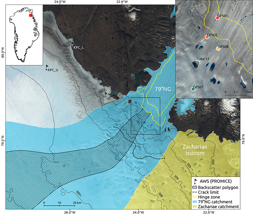
Figure 1. Overview of the study area. Hatched polygon marks the area used for the backscatter analysis shown in Figure 2b. Catchment areas are from Krieger et al. (2020). Inlet shows the locations of GPS receivers shown in Figure 3 and Figure S2. KPC_U and KPC_L are the closest Automatic Weather Stations (AWS) from the PROMICE project (Fausto and van As, 2019). In the background is a Sentinel-2 acquisition from 28 July 2017. Hinge zone is determined from ERS-II SAR interferometry, data were acquired in April/May 2011. Upper limit of major crevasses is shown as dashed black line.

2. Seasonal Melt Patterns

To obtain information as to when the melt season starts, for how long it lasts and to what altitude surface melt can be expected we extracted a dense time series of backscatter values from the Sentinel-1 archive. Sentinel-1A was launched on 3 April 2014, followed by its twin satellite Sentinel-1B on 25 April 2016. Both satellites are equipped with a C-band Synthetic Aperture Radar (SAR) sensor with a shifted repeat cycle of 12 days, resulting in a 6 day revisiting time when both satellites are employed. In this study we used numerous Level-1 Single Look Complex (SLC) products obtained in Interferometric Wide swath (IW) mode. The data were acquired between January 2015 and January 2019 in relative orbit 74 over the study area. Following the suggestions of Winsvold et al. (2018) we build our analysis on a time series of the terrain corrected backscatter coefficient gamma nought (γ⁰). The processing includes calibrating, mosaicing and multi-looking of the TOPS SAR data followed by a terrain correction and geocoding step. Radiometric calibration was done within the GAMMA^® software resulting in σ⁰ backscatter values using the ellipsoid area as reference area for normalization. Subsequently all bursts of each acquisition were mosaiced into a continuous SLC image. In order to reduce noise, multi-looking was performed with 10 looks in range direction and 2 looks in azimuth direction. To obtain terrain corrected γ⁰ values we applied an additional reference area normalization based on the ArcticDEM, gridded to 100 m spatial resolution (Small, 2011; Porter et al., 2018). Finally, all SAR images were geocoded and linear backscatter values were translated to decibels.

Backscatter values returned from glaciers and ice sheets heavily depend on instrument related parameters such as incidence angle and polarization as well as on characteristics of the upper surface layers such as roughness, water content, snow density, grain size and impurities (e.g., Rau and Braun, 2002; Winsvold et al., 2018). As wet snow absorbs most of the SAR signal, low surface scattering prevails in these areas, allowing to discriminate between wet and frozen zones on a glacier.

In order to estimate the onset and duration of surface melt we employed the binned backscatter values (γ⁰) from the time series shown in Figure 2b. Following QSCAT scatterometer studies over Greenland (e.g., Wang et al., 2007) we compared all γ⁰ values to the mean γ⁰ of the respective altitude band for December, January and February of the previous winter (Wγ⁰). If γ⁰ drops below Wγ⁰−3dB the respective bin is treated as surface melt and is marked by a black dot in Figure 2b. Due to larger data gaps and a 12-day repeat pass in 2015 and 2016 confident interpretations can only be made for 2017 and 2018. In 2017 the onset of surface melt is set to 2 June and lasts until 6 September (96 days) where isolated surface melt is found at low elevations of <250 m. At the other end of the scale surface melt reaches elevations of almost 1750 m on 1 August 2017 (Figure 2b and Video S1). In 2018 surface melt starts on 15 June and ends on 7 September (84 days). Similar to 2017 the maximum extent of surface melt is found on 2 August, while isolated patches are found at low elevations until September 2018 (Figure 2b and Video S1). Due to the 6-day repeat pass of Sentinel-1 these estimates might be underestimated by up to 10 days in the most unfavorable case.

FIGURE 2

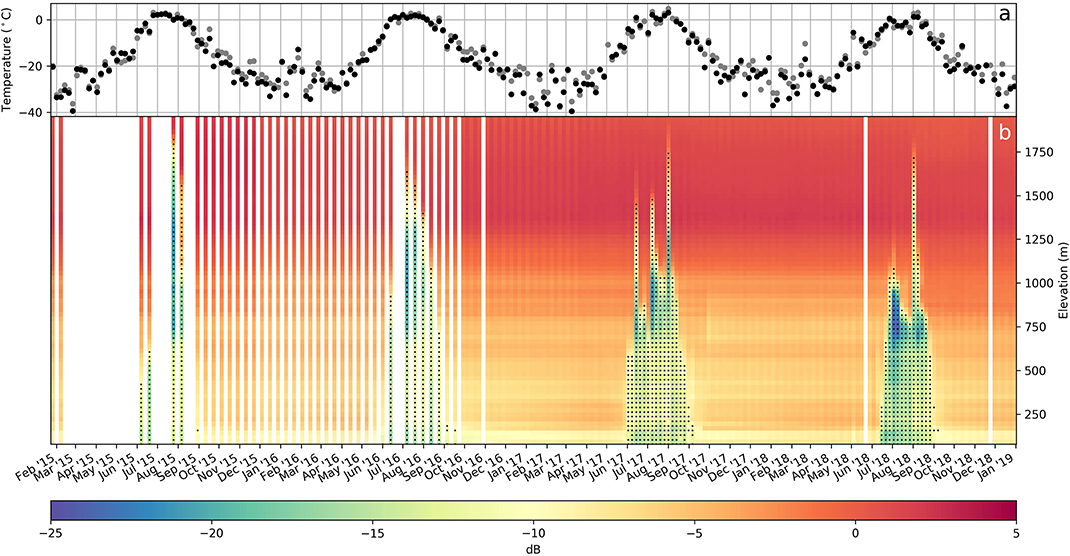
Figure 2. Near surface air temperature measured at PROMICE AWS KPC_U (Fausto and van As, 2019, Figure 1, black dots) and ERA5 2 m air temperature reanalysis estimates at the same location (Hersbach and Dee, 2016, gray dots, (a)). Heat plot of Sentinel-1 backscatter coefficient γ⁰ time series (b). Data are extracted from the hatched polygon shown in Figure 1 and binned to 25 m elevation classes. Bins with surface melt are marked by small black dots.

As surface melt heavily depends on air temperature, we additionally employed temperature data from nearby Automatic Weather Stations (AWS) as well as from the recently released ERA5 reanalysis dataset (Hersbach and Dee, 2016). Here we used daily averages of near surface air temperature acquired by AWS KPC_L and KPC_U of the Programme for Monitoring the Greenland Ice Sheet (PROMICE) (Fausto and van As, 2019). KPC_L and KPC_U are located at an altitude of 370 and 870 m, respectively and their positions are marked in Figure 1. At the position of KPC_U we also extracted 2 m air temperature data from the ERA5 reanalysis dataset (Figure 2a). ERA5 reanalysis data are available at a spatial resolution of 0.25° and it is worthwhile noting that PROMICE observations are not assimilated in the reanalysis dataset (Delhasse et al., 2020). Between ERA5 2 m air temperature data and KPC_U near surface air temperature data we found a squared correlation coefficient of 0.98 when investigating the time interval shown in Figure 2a (Figure S1).

3. Surface Velocities

Horizontal surface velocities were obtained by GPS measurements and intensity offset tracking on high resolution TerraSAR-X stripmap data. In summer 2017 four autonomous GPS stations were installed near the hinge zone of 79°N Glacier (Figure 1). All GPS stations included one state-of-the-art Novatel FlexPak6 L-Band GPS receiver, one Novatel choke ring GPS antenna, at least one data logger, two solar panels, one solar charge controller and two 105 Ah batteries. The antennas were mounted on aluminum tripods and fixed to the ice by additional weights and long nails. GPS data were logged every 15 s and were processed using Precise Point Positioning (PPP) processing implemented in the Waypoint^® software including final precise international GNSS Service ephemerides. Velocities were calculated based on horizontal displacements within a 24 h moving window over all measurements. Each velocity estimate was then allocated to the center time of the moving window. Finally, average velocities were calculated for each day to obtain an overview of the general velocity pattern shown in Figures 3b–e. In order to detect short term variations in ice velocities (<1 d) related to e.g., lake drainage we produced an additional dataset using a 4 h moving window with no daily averaging (Figure S2). The standard deviation of the horizontal displacement is estimated with <5 mm for all stations. This results in a velocity error of up to 0.06 and 0.01 m d⁻¹ for the 4 and 24 h moving window, respectively.

FIGURE 3

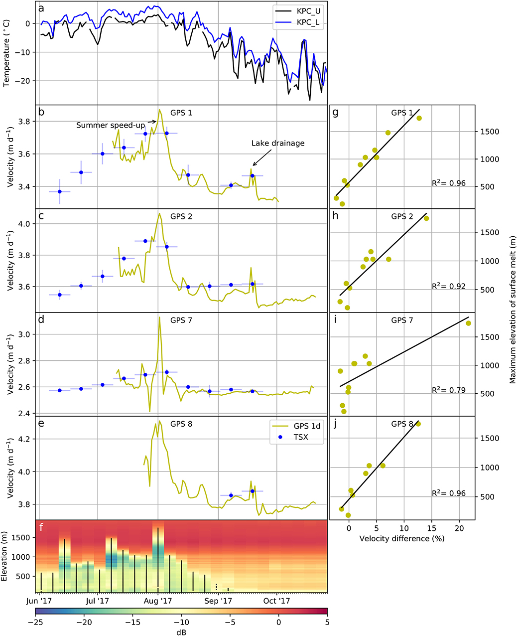
Figure 3. Relation between near surface air temperature measured at PROMICE AWS KPC_U and KPC_L (a) (Fausto and van As, 2019), horizontal surface velocities as measured at the four GPS sites indicated in Figure 1 (b–e) and surface melt estimates from the Sentinel-1 time series shown in Figure 2b (f). TerraSAR-X derived surface velocities are centered at the mean date between data acquisitions with light blue bars in x-direction indicating the 11-day period between the dates of data acquisition. Light blue bars in y-direction represent the weighted standard deviation of the pixel values employed in the interpolation of the shown velocity estimates. GPS estimates are averaged over one day. Note the different data ranges in (b–e). Scatter plots (g–j) show the relation between GPS measured surface velocities relative to a TerraSAR-X derived winter velocity field and the maximum elevation of surface melt from the Sentinel-1 time series shown in Figure 2b and (f).

We further obtained velocity fields from TerraSAR-X intensity offset tracking for a similar time period. The processing includes co-registration of SLC data separated by 11 days followed by cross correlating the backscatter intensity of each SLC pair in a predefined moving search window (e.g., Strozzi et al., 2002). Following Rückamp et al. (2019) we chose a window size of 250 m in both range and azimuth direction with a step size of 50 m. Range and azimuth offsets were then projected into a polar stereographic coordinate system assuming surface parallel ice flow. Surface velocity fields were filtered following the three step filtering approach described by Lüttig et al. (2017). This approach is designed to efficiently detect outliers in surface velocity fields and is based on 1. a segmentation filter which is based on the assumption that velocity fields can be divided into segments of continuous ice flow (Rosenau et al., 2015), 2. anomalies to a running median and 3. variations of flow directions within a moving search window. Finally, all velocity fields were gridded to 250 m and small data gaps were interpolated with an inverse distance weighting scheme. The latter step was applied since surface velocities were calculated during the melt season where the presence of water strongly modifies the radar backscatter resulting in rather noisy velocity estimates and data gaps. However, as our GPS receivers are located in the central part of the ice stream we expect only small variations in the ice velocities of adjacent flowlines, suggesting a lower sensitivity toward grid resolution when compared to e.g., shear margins (Joughin et al., 2018). As a measure of confidence we included the weighted standard deviation of the pixel values employed in the inverse distance interpolation of the velocity estimates shown in Figures 3b–e.

Overall the TerraSAR-X derived velocities are in good agreement with the GPS derived velocities (Figures 3b–e). By combining both datasets we found that surface velocities at the four GPS sites start to increase from their winter baseline in early June and are peaking at the end of July / beginning of August 2017 (annotated as summer speed-up in Figure 3b). However, velocity estimates derived from GPS data are resolved to a higher temporal resolution than those from intensity offset tracking (1 vs. 11 d). Therefore, a greater amount of detail can be observed in the GPS derived dataset. While all GPS receivers show highest surface velocities on 1 August 2017 this peak is averaged out in the TerraSAR-X estimates leading to slower summer velocities. Depending on the dataset and the location, summer acceleration can be up to 22% for the GPS and 9% for the TerraSAR-X derived estimates, respectively. Since we lack winter velocities from the GPS stations due to power limitations, all relative velocity changes throughout this study are referenced to the corresponding pixel values of a TerraSAR-X winter velocity field with data acquired on 10 and 21 December 2017 (not shown in Figure 3b–e). In order to detect the upper spatial limit of seasonally enhanced flow velocities we calculated differences between all TerraSAR-X velocity fields and the winter 2017 reference field Figure 6). If possible we also computed GPS derived velocity estimates specific to each 11-day time period of the TerraSAR-X estimates. Here we found similar values as from the intensity offset tracking with a summer acceleration of up to 7% when compared to the December TerraSAR-X velocity field.

After returning to their approximate winter baseline in late August all GPS receivers show a simultaneous speed-up in late September which is significantly lower in the record of GPS 7 (annotated as lake drainage in Figure 3b, a close-up is shown in Figure S2). Directly after this second velocity peak, velocities remain under their winter baseline for several days, until they slowly start to increase again.

4. Lake Drainage

To explain the unusual speed-up observed in September 2017, we carefully checked radar and optical satellite acquisitions in this time period. Between 18 and 19 September 2017 we found a sudden drainage of supraglacial lake 11 (name originates from arbitrary indexing of supraglacial lakes in the area, lake position is at −22.978°E, 79.338°N, Figure 1) on cloud free Sentinel-2 imagery (Figures 4b,c). In order to obtain an estimate of the drainage volume we further generated two Digital Elevation Models (DEMs) from bistatic TanDEM-X data acquired on 13 and 24 September 2017 following the methods described by Neckel et al. (2013). Both DEMs were vertically adjusted to the same reference DEM by removing a linear trend estimated over stable bedrock. Pixel-by-pixel DEM differences were calculated on the same spatial grid with a resolution of 10 m. The elevation differences are shown in Figure 4d and show a subsidence of >50 m in the center of the lake. Finally, elevation changes were translated into drainage volume by

$\begin{array}{ll}{V}_{drain}={\displaystyle \sum _{i=0}^n}{(\Delta h^{lake}{p}^2)}_i,if\Delta h_i^{lake}<-1& (1)\end{array}$

where Δh^lake are the elevation changes within manually digitized shorelines, and p is the pixel size which was set to 100 m to reduce noise. In order to solely employ Δh^lake values of elevation loss, we introduced a threshold of -1 m in the calculation of V_drain. Following Equation 1 we estimated a volume of 28 × 10⁶ m³ for this drainage event. Almost 2 month before on 21 July 2017 we installed a data logger at this specific lake with the intention to autonomously record water pressure and temperature. Unfortunately, the data logger could not be recovered in 2018 but was probably lost during the rapid drainage event in September 2017. However, when installing the logger we measured a lake depth of 10.80 m at the location marked by the yellow dot in Figure 4a (Figure S2). This value fits well to the TanDEM-X derived elevation difference of -11.05 m at the exact location.

FIGURE 4

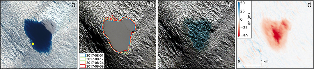
Figure 4. Rapid drainage event (<24 h) of lake 11 in September 2017. Sentinel-2 acquisition on 17 August 2017 at 15:09 is shown in (a), lake is mostly ice free, yellow dot marks the location of lake depth measurement on 21 July 2017 (Figure S2). Sentinel-2 acquisition on 18 September 2017 at 15:49 is shown in (b), lake is completely covered by lake ice. Additional pre-drainage shorelines are shown. Note the difference in illumination between August and September. Sentinel-2 acquisition on 19 September 2017 at 15:18 is shown in (c), the lake has drained and is not covered by ice anymore. TanDEM-X derived surface elevation changes between 13 and 24 September 2017 are shown in (d).

5. Discussion

By analyzing a dense time series of Sentinel-1 γ⁰ backscatter coefficients in relation to surface elevation we obtained a good overview of when the melt season starts and to what altitude surface melt can be expected (Figure 2b). Also a clear correlation between surface melt and near surface air temperature is found when including additional meteorological datasets in the analysis (Figure 2a). Focusing on the time with surface velocity measurements, we find that in June, July and August 2017 surface melt is detected generally to elevations between 600 and 1,000 m with short term excursions reaching elevations >1,250 m. During the melt onset on 2 June 2017 surface melt reaches rather low elevations of 580 m, which is also reflected in the AWS data shown in Figure 3a. While the higher elevated KPC_U station measured the first positive degree day on 10 June 2017, i.e., 8 days after the detected melt onset, KPC_L recorded the first positive degree day contemporaneous on 1 June 2017. Having in mind that our GPS receivers are located at elevations between 70 and 390 m we conclude that melt water was available during the entire 3 month period in this region. A general increase in surface velocities is observed at all four GPS stations prior to August 2017 (Figures 3b–e). Also from our backscatter analysis we detected the largest extent of surface melt at this time reaching elevations of almost 1750 m on 1 August 2017 (Figures 2b, 3f). The temporal coexistence of peaks in surface velocities of all GPS receivers to this date is quite striking and suggests a strong and direct reaction of surface velocities to the availability of melt water. At this time also the highest daily mean near-surface air temperatures of +3.1 and +6.1°C were measured at KPC_U and KPC_L, respectively, underpining that surface melt is largely driven by air temperature (Figure 3a). This is further supported by ERA5 reanalysis data where a significant anomaly is found when comparing the average 2 m air temperature of 1 August 2017 to the monthly average of July 2017 (Figure 5a, Hersbach and Dee, 2016). Also the 0°C isotherm on 1 August 2017 matches quite well with the upper limit of surface melt as detected from the backscatter time series (Figure 5a). When investigating the scatter plots shown in Figures 3g,h it is likely that the larger the area affected by surface melt is the stronger the velocity response downstream the glacier. However, the question remains how the melt water is speeding up the glacier. In line with recent work by Rathmann et al. (2017) and Vijay et al. (2019) who also found a direct velocity response of 79°N Glacier to the occurrence of surface melt, we suggest that surface melt water reaches the ice-bed interface quite quickly through predefined pathways such as cracks and crevasses. This is supported when investigating the spatial distribution of seasonal glacier speed-up as shown in Figure 6. Here the dashed black line marks the upper limit of major crevasses which was delineated with the help of several TerraSAR-X acquisitions. With an average altitude of 680 m this upper crack limit lies at the lower limit of the estimated melt extent shown in Figure 2b. Even in the time period of the largest melt extent (Figure 2b) and the highest ice acceleration (Figures 6D–F) significant changes in surface speed stayed well below this line. This suggests that the melt water from higher elevated regions is routed on the ice surface until it reaches the crevassed zone at lower elevations. Here the water is quickly routed to the ice-bed interface through numerous cracks and crevasses and is acting as a lubricant for the overlaying ice column causing a seasonal acceleration of the ice stream. For the Greenland Ice Sheet such mechanisms were first described by Zwally et al. (2002) but were previously known also for mountain glaciers (e.g., Iken et al., 1983).

FIGURE 5

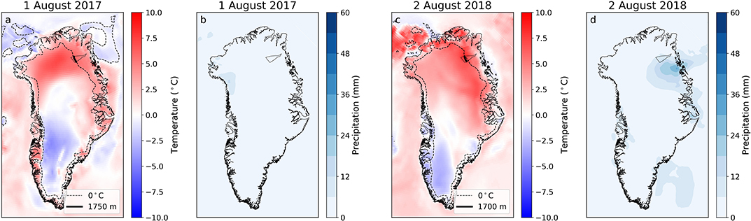
Figure 5. ERA5 reanalysis data for selected dates with high surface melt. 2 m air temperature anomaly of 1 August 2017 vs. the monthly average of July 2017 is shown in (a), together with the 0°C isotherm and the maximum altitude of surface melt on 1 August 2017 (1750 m). Cumulated hourly precipitation of 1 August 2017 is shown in (b). Panels (c,d) show the same as (a) and (b) but for 2 August 2018. The polygon framed by a black solid line marks the area used for the backscatter analysis shown in Figure 2b.

FIGURE 6

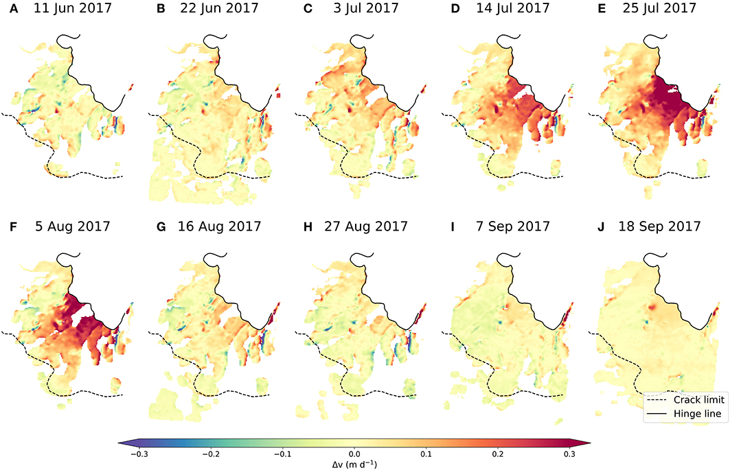
Figure 6. Increase (A–F) and decrease (G–J) in 2017 surface velocities upstream the hinge line (solid black line) of 79°N Glacier when compared to winter velocities of the same year. Dates are the center dates between the 11-day repeat pass of TerraSAR-X employed in the generation of the summer velocity fields. Winter velocites were derived from TerraSAR-X data acquired between 10 December 2017 and 21 December 2017.

After the velocity peak in the beginning of August 2017 velocities started to decrease again accompanied by a decrease in melt extent and air temperature (Figures 3a–f). Then a second speed-up was recorded by our GPS receivers in September 2017 where no surface melt can be detected from the backscatter time series and near-surface air temperatures measured at KPC_U and KPC_L stayed well below 0°C (Figure 3a). This second speed-up can clearly be attributed to a rapid drainage event of lake 11 between 18 and 19 September 2017. While the lake was completely covered by lake ice on 18 September 2017 no ice layer was present on 19 September 2017 and the lake area significantly decreased in less than 24 h (Figure 4b,c). We therefore conclude, that the lake drainage started at some point close to 18 September 2017 and the lake ice broke up due to the drainage event. Considering the short time period of the lake drainage, water-driven fracture propagation seems to be the most likely mechanism to establish a connection to the bed (e.g. Das et al., 2008). While GPS 1, 2, and 8 received a similar signal on 19 September only a minor speed-up was recorded by GPS 7 which is located upstream of lake 11 (Figures 1, 3b–e). This implies that the water, with an estimated volume of 28 × 10⁶ m³ was not routed through established channels but overwhelmed the subglacial hydraulic system and spread along the ice-bed interface downstream of lake 11. Here ice velocities increased by up to 24% when compared to pre-drainage velocities (Figure S2). This is in contrast to other studies which report post-drainage ice velocities of 4–10 times larger than before a rapid lake drainage event (e.g., Hoffman et al., 2011; Tedesco et al., 2013). These differences are most likely attributed to the comparatively large distances of our GPS receivers to the lake. While Tedesco et al. (2013) report distances within 2 km of the lake and receiver locations along flowlines through the lake, our GPS receivers are located between 6.5 and 12.5 km from the lake and do not match any flowline through the lake (Figure 1). Further, it has been shown that changes in water supply are key for driving ice accelerations rather than the absolute amount of water input (e.g., Schoof, 2010; Bartholomew et al., 2012). This might explain why the relatively large drainage volume has only a limited effect on the ice dynamics in the area.

When focusing our backscatter time series on the melt season 2018, we find indirect evidence for a cold summer with high levels of precipitation as described elsewhere (Polar Portal Season Report, 2018). Compared to 2017 the melt season started almost 2 weeks later on 15 June 2018. The largest extent of surface melt is found on 2 August 2018 where it reaches a similar altitude as on 1 August 2017 (Figures 2b, 5c). While compared to 1 August 2017 lower values of daily mean near-surface air temperature of +1.4 and +3.2°C were measured at KPC_U and KPC_L, respectively, precipitation might have enhanced surface melt and/or accumulated in the upper snow layers. At this day no helicopter supported field work was possible due to rainy conditions with low clouds and also ERA5 reanalysis data suggests precipitation in the area (Figure 5d). This is in contrast to 1 August 2017 were dry conditions can be assumed (Figure 5b). So far no GPS measurements are available for 2018 but it has been shown previously, that precipitation can have a direct influence on glacier velocities (Doyle et al., 2015).

The results presented in this study are in general agreement with the findings of Rathmann et al. (2017) who also suggest that the seasonal speed-up of 79°N Glacier is largely driven by surface melt water lubricating the bed. By conducting modeling experiments, Rathmann et al. (2017) rule out other potential drivers such as seasonally enhanced sliding along the side walls of the floating tongue. For recent ice flow conditions Mayer et al. (2018) asses a strong buttressing effect of the floating ice tongue, especially within the narrower part of Nioghalvfjerd fjord (i.e., for the first ~30 km downstream the floating part of the ice tongue). This implies a low sensitivity of seasonal ice velocities toward varying sea ice conditions, an assumption which can not be made for the neighboring ZachariæIsstrom. For the latter Rathmann et al. (2017) find that the break up of the ice mélange coincides with the onset of surface melt upstream the glacier, making a distinction of processes governing the seasonal ice acceleration rather difficult. When investigating 45 Greenlandic glaciers, Vijay et al. (2019) could link the seasonal varying surface velocities of roughly half of them to surface melt induced changes of the subglacial hydrology. For less than a quarter of their study glaciers, Vijay et al. (2019) found a correlation between seasonal ice velocities and terminus changes. Even though surface melt water might also play a role in the seasonal velocity evolution of the latter group, Moon et al. (2014) suggest that fluctuations in terminus position are the primary controlling factor for these glaciers. According to the classification scheme introduced by Moon et al. (2014) and Vijay et al. (2019), 79°N Glacier fits well within their type 2 behavior by showing a strong correlation between glacier velocity and runoff. This also implies that a seasonal development of an efficient channelized subglacial drainage system is rather limited for 79°N Glacier.

While the above studies are solely based on remotely sensed surface velocities, we show that by the additional use of GPS measurements short term velocity variations are preserved which would be averaged out if only remote sensing estimates were available. Based on intensity offset tracking on Sentinel-1 data, Lemos et al. (2018) and Rathmann et al. (2017) found a seasonal acceleration of 79°N Glacier by 10 and 11%, respectively. These estimates match comparably well with our estimate of 9% based on TerraSAR-X data, even though sampling location, time stamp and reference data were different in all three studies. Such velocity estimates might be sufficient for monthly averaged mass balance estimates or general trends in seasonal velocity behavior, but short term velocity fluctuations with rather low amplitudes are difficult to quantify from the current satellite missions with temporal baselines of several days.

6. Conclusions

By combining remote sensing observations with in situ GPS measurements we were able to link the occurrence of extensive surface melt to a direct velocity response of 79°N Glacier. While we found a maximum seasonal velocity increase of 22% from GPS measurements, these average out to 9% when velocities are calculated over longer time intervals such as the 11-day repeat pass of TerraSAR-X. We therefore conclude, that surface velocities derived by remote sensing give a good overview over entire seasons or major speed-up events, but are not able to fully resolve short term velocity fluctuations triggered by e.g., rapid lake drainage events. For the latter we found an example even after the melt season in mid September when temperatures were well below 0°C. By utilizing digital elevation models from the TanDEM-X satellite mission we were able to estimate a drainage volume of 28 × 10⁶ m³ which resulted in a minor speed-up of 24% when compared to pre-drainage ice velocities estimated from 3 GPS stations downstream the lake. Compared to studies in western Greenland the observed speed up is a magnitude lower. On the one hand this can be attributed to the large distances of our GPS receivers to the lake, on the other hand this could possibly support findings that not the amount of water is decisive for ice acceleration but rather the timing and the changes in water supply in combination with the effectivity of the hydraulic system.

Data Availability Statement

The datasets generated for this study are available on request to the corresponding author.

Author Contributions

NN processed and analyzed the remote sensing data and wrote the initial draft of the manuscript. OZ and VH processed the GPS data. NN, OZ, and DS conducted field work. AH designed the project, lead the field program and supervised the study. All authors continuously discussed the results.

Funding

This project has received funding from the European Union's Horizon 2020 research and innovation programme under grant agreement No 689443 via project iCUPE (Integrative and Comprehensive Understanding on Polar Environments). OZ received founding through BMBF Project GROCE (03F0778A).

Conflict of Interest

The authors declare that the research was conducted in the absence of any commercial or financial relationships that could be construed as a potential conflict of interest.

Acknowledgments

TanDEM-X and TerraSAR-X data were made available through German Aerospace Center proposals GLAC7208 and HYD2059. Data from the Programme for Monitoring of the Greenland Ice Sheet (PROMICE) were provided by the Geological Survey of Denmark and Greenland (GEUS) at http://www.promice.dk. We want to thank Jens Köhler and Graham Niven for their help in the field.

Supplementary Material

The Supplementary Material for this article can be found online at: https://www.frontiersin.org/articles/10.3389/feart.2020.00142/full#supplementary-material

References

Bartholomew, I., Nienow, P., Mair, D., Hubbard, A., King, M. A., and Sole, A. (2010). Seasonal evolution of subglacial drainage and acceleration in a Greenland outlet glacier. Nat. Geosci. 3:408. doi: 10.1038/ngeo863

CrossRef Full Text | Google Scholar

Bartholomew, I., Nienow, P., Sole, A., Mair, D., Cowton, T., and King, M. A. (2012). Short-term variability in Greenland Ice Sheet motion forced by time-varying meltwater drainage: implications for the relationship between subglacial drainage system behavior and ice velocity. J. Geophys. Res. Earth Surf . 117. doi: 10.1029/2011JF002220

CrossRef Full Text | Google Scholar

Das, S. B., Joughin, I., Behn, M. D., Howat, I. M., King, M. A., Lizarralde, D., et al. (2008). Fracture propagation to the base of the greenland ice sheet during supraglacial lake drainage. Science 320, 778–781. doi: 10.1126/science.1153360

PubMed Abstract | CrossRef Full Text | Google Scholar

Delhasse, A., Kittel, C., Amory, C., Hofer, S., van As, D., and S. Fausto, R. (2020). Brief communication: evaluation of the near-surface climate in ERA5 over the Greenland Ice Sheet. Cryosphere 14, 957–965. doi: 10.5194/tc-14-957-2020

CrossRef Full Text | Google Scholar

Doyle, S. H., Hubbard, A., van de Wal, R. S. W., Box, J. E., van As, D., Scharrer, K., et al. (2015). Amplified melt and flow of the Greenland ice sheet driven by late-summer cyclonic rainfall. Nat. Geosci. 8:647. doi: 10.1038/ngeo2482

CrossRef Full Text | Google Scholar

Fausto, R., and van As, D. (2019). Programme for Monitoring of the Greenland Ice Sheet (PROMICE): Automatic Weather Station Data. Version: v03. doi: 10.22008/promice/data/aws

CrossRef Full Text | Google Scholar

Hersbach, H., and Dee, D. (2016). ERA5 reanalysis is in production. ECMWF Newslett. 147:7.

Google Scholar

Hoffman, M. J., Catania, G. A., Neumann, T. A., Andrews, L. C., and Rumrill, J. A. (2011). Links between acceleration, melting, and supraglacial lake drainage of the western Greenland Ice Sheet. J. Geophys. Res. Earth Surf. 116:16. doi: 10.1029/2010JF001934

CrossRef Full Text | Google Scholar

Igneczi, d., Sole, A. J., Livingstone, S. J., Leeson, A. A., Fettweis, X., Selmes, N., et al. (2016). Northeast sector of the Greenland ice sheet to undergo the greatest inland expansion of supraglacial lakes during the 21st century. Geophys. Res. Lett. 43, 9729–9738. doi: 10.1002/2016GL070338

CrossRef Full Text | Google Scholar

Iken, A., Rothlisberger, H., Flotron, A., and Haeberli, W. (1983). The uplift of unteraargletscher at the beginning of the melt season - a consequence of water storage at the bed? J. Glaciol. 29, 28–47. doi: 10.1017/S0022143000005128

CrossRef Full Text | Google Scholar

Joughin, I., Das, S. B., Flowers, G. E., Behn, M. D., Alley, R. B., King, M. A., et al. (2013). Influence of ice-sheet geometry and supraglacial lakes on seasonal ice-flow variability. Cryosphere 7, 1185–1192. doi: 10.5194/tc-7-1185-2013

CrossRef Full Text | Google Scholar

Joughin, I., Smith, B. E., and Howat, I. (2018). Greenland Ice Mapping Project: ice flow velocity variation at sub-monthly to decadal timescales. Cryosphere 12, 2211–2227. doi: 10.5194/tc-12-2211-2018

CrossRef Full Text | Google Scholar

Krieger, L., Floricioiu, D., and Neckel, N. (2020). Drainage basin delineation for outlet glaciers of Northeast Greenland based on Sentinel-1 ice velocities and TanDEM-X elevations. Remote Sens. Environ. 237:111483. doi: 10.1016/j.rse.2019.111483

CrossRef Full Text | Google Scholar

Lemos, A., Shepherd, A., McMillan, M., Hogg, A. E., Hatton, E., and Joughin, I. (2018). Ice velocity of Jakobshavn Isbræ, Petermann Glacier, Nioghalvfjerdsfjorden, and Zachariæ Isstrøm, 2015-2017, from Sentinel 1-a/b SAR imagery. Cryosphere 12, 2087–2097. doi: 10.5194/tc-12-2087-2018

CrossRef Full Text | Google Scholar

Lüttig, C., Neckel, N., and Humbert, A. (2017). A combined approach for filtering ice surface velocity fields derived from remote sensing methods. Remote Sens. 9:23. doi: 10.3390/rs9101062

CrossRef Full Text | Google Scholar

Mayer, C., Schaffer, J., Hattermann, T., Floricioiu, D., Krieger, L., Dodd, P. A., et al. (2018). Large ice loss variability at Nioghalvfjerdsfjorden Glacier, Northeast-Greenland. Nat. Commun. 9:2768. doi: 10.1038/s41467-018-05180-x

PubMed Abstract | CrossRef Full Text | Google Scholar

Moon, T., Joughin, I., Smith, B., van den Broeke, M. R., van de Berg, W. J., Noel, B., et al. (2014). Distinct patterns of seasonal Greenland glacier velocity. Geophys. Res. Lett. 41, 7209–7216. doi: 10.1002/2014GL061836

PubMed Abstract | CrossRef Full Text | Google Scholar

Neckel, N., Braun, A., Kropáček, J., and Hochschild, V. (2013). Recent mass balance of the Purogangri Ice Cap, central Tibetan Plateau, by means of differential X-band SAR interferometry. Cryosphere 7, 1623–1633. doi: 10.5194/tc-7-1623-2013

CrossRef Full Text | Google Scholar

Polar Portal Season Report (2018). Available online at: http://polarportal.dk/en/news/2018-season-report/

Google Scholar

Porter, C., Morin, P., Howat, I., Noh, M.-J., Bates, B., Peterman, K., et al. (2018). ArcticDEM, Harvard Dataverse, V1. doi: 10.7910/DVN/OHHUKH

CrossRef Full Text | Google Scholar

Rathmann, N. M., Hvidberg, C. S., Solgaard, A. M., Grinsted, A., Gudmundsson, G. H., Langen, P. L., et al. (2017). Highly temporally resolved response to seasonal surface melt of the Zachariae and 79N outlet glaciers in northeast Greenland. Geophys. Res. Lett. 44, 9805–9814. doi: 10.1002/2017GL074368

CrossRef Full Text | Google Scholar

Rau, F., and Braun, M. (2002). The regional distribution of the dry-snow zone on the Antarctic Peninsula north of 70°S. Ann. Glaciol. 34, 95–100. doi: 10.3189/172756402781817914

CrossRef Full Text | Google Scholar

Rosenau, R., Scheinert, M., and Dietrich, R. (2015). A processing system to monitor Greenland outlet glacier velocity variations at decadal and seasonal time scales utilizing the Landsat imagery. Remote Sens. Environ. 169, 1–19. doi: 10.1016/j.rse.2015.07.012

CrossRef Full Text | Google Scholar

Rückamp, M., Neckel, N., Berger, S., Humbert, A., and Helm, V. (2019). Calving induced speedup of Petermann glacier. J. Geophys. Res. Earth Surf. 124, 216–228. doi: 10.1029/2018JF004775

CrossRef Full Text | Google Scholar

Schoof, C. (2010). Ice-sheet acceleration driven by melt supply variability. Nature 468:803. doi: 10.1038/nature09618

PubMed Abstract | CrossRef Full Text | Google Scholar

Small, D. (2011). Flattening gamma: radiometric terrain correction for SAR imagery. IEEE Trans. Geosci. Remote Sens. 49, 3081–3093. doi: 10.1109/TGRS.2011.2120616

CrossRef Full Text | Google Scholar

Strozzi, T., Luckman, A., Murray, T., Wegmuller, U., and Werner, C. (2002). Glacier motion estimation using SAR offset-tracking procedures. IEEE Trans. Geosci. Remote Sens. 40, 2384–2391. doi: 10.1109/TGRS.2002.805079

CrossRef Full Text | Google Scholar

Tedesco, M., Willis, I. C., Hoffman, M. J., Banwell, A. F., Alexander, P., and Arnold, N. S. (2013). Ice dynamic response to two modes of surface lake drainage on the Greenland ice sheet. Environ. Res. Lett. 8:034007. doi: 10.1088/1748-9326/8/3/034007

CrossRef Full Text | Google Scholar

Vijay, S., Khan, S. A., Kusk, A., Solgaard, A. M., Moon, T., and Bjork, A. A. (2019). Resolving seasonal ice velocity of 45 greenlandic glaciers with very high temporal details. Geophys. Res. Lett. 46, 1485–1495. doi: 10.1029/2018GL081503

CrossRef Full Text | Google Scholar

Wang, L., Sharp, M., Rivard, B., and Steffen, K. (2007). Melt season duration and ice layer formation on the Greenland ice sheet, 2000-2004. J. Geophys. Res. Earth Surf. 112:15. doi: 10.1029/2007JF000760

CrossRef Full Text | Google Scholar

Winsvold, S. H., Kääb, A., Nuth, C., Andreassen, L. M., van Pelt, W. J. J., and Schellenberger, T. (2018). Using SAR satellite data time series for regional glacier mapping. Cryosphere 12, 867–890. doi: 10.5194/tc-12-867-2018

CrossRef Full Text | Google Scholar

Zwally, H. J., Abdalati, W., Herring, T., Larson, K., Saba, J., and Steffen, K. (2002). Surface melt-induced acceleration of Greenland ice-sheet flow. Science 297, 218–222. doi: 10.1126/science.1072708

PubMed Abstract | CrossRef Full Text | Google Scholar