Numerical Modeling Shows Increased Fracturing Due to Melt-Undercutting Prior to Major Calving at Bowdoin Glacier

1. Introduction

Marine-terminating outlet glaciers of the Greenland Ice Sheet thin, accelerate and retreat faster than any other part of the ice sheet (e.g., Pritchard et al., 2009; Hill et al., 2017). The Greenland Ice Sheet lost 1, 827±538 Gt of ice due to glacier discharge from 1992 to 2018, accounting for 48% of the total mass loss (IMBIE Team, 2019). Future mass loss predictions, and thereby sea level rise predictions, are strongly affected by the representation of marine-terminating outlet glaciers in numerical ice sheet models (Catania et al., 2019; Goelzer et al., 2020). Up to 40% of the uncertainty of sea level rise projections is caused by the uncertainty in calving parameterizations (Bulthuis et al., 2019). Despite recent major advances in modeling calving, it remains challenging to formulate a robust calving law for ice sheet models that calculates mass loss induced by the range of observed calving styles (Benn and Åström, 2018). Since calving is the mechanical detachment of icebergs from the glacier terminus, the location and timing of calving events are determined by fracture initiation and propagation (Benn et al., 2007). Fractures in the ice are both influenced by and affect the stress state of glaciers (Colgan et al., 2016). This interconnection contributes to the complexity of parameterizing calving in large-scale ice sheet models.

Additionally, several physical processes that are known to affect iceberg calving are poorly constrained by observations (Benn et al., 2007). This is particularly the case for calving associated with submarine melting of the ice front, because melting and calving processes are not independent. Melt-induced undercutting of termini may cause an increase in calving by altering stresses up- or across-glacier, a so-called “calving amplifier” effect (O'Leary and Christoffersen, 2013; Benn et al., 2017; Cowton et al., 2019). However, confirming such an effect is difficult since directly observing both submarine calving and melt rates is challenging. Estimated melt rates rely on modeling or hydrographic data taken at a distance from the glacier terminus (Slater et al., 2016). Using these methods, submarine melt rate estimates range from 0.7 to 10 m d⁻¹ for Greenland (Rignot et al., 2010; Sutherland and Straneo, 2012; Xu et al., 2013; Inall et al., 2014). Where glacier runoff reaches the calving front through channels below sea level, buoyant plumes appear that entrain relatively warm seawater and thereby increase submarine melt locally (Jenkins, 2011). Ambient melt, outside of such plumes, was previously thought to be insignificant compared to plume-driven melt (Cowton et al., 2015; Carroll et al., 2016). However, repeat multibeam surveying-derived ambient melt rates are as high as ~5 m d⁻¹ at LeConte Glacier, Alaska (Jackson et al., 2020), two orders of magnitude higher than predicted by existing plume-melt parameterizations (Jenkins, 2011; Cowton et al., 2015). Therefore, the relative importance of distributed and localized melt and their effect on calving is still unclear.

Besides measuring melt rates, observing submarine glacier front geometries is also challenging. Rare geometry observations have shown that a plume can cause a locally undercut glacier front, with undercut lengths into the glacier that can be as large as the water depth (Fried et al., 2015; Rignot et al., 2015; How et al., 2019). Fried et al. (2015) found that 80% of the terminus of a West Greenland glacier is undercut and they observed many deeply-undercut outlets even for subsurface plumes with small discharge fluxes. Cowton et al. (2019) showed that the location of such local undercuts determines whether submarine melt can act as a calving amplifier. Their model study shows that localized melting near the lateral margins might trigger increased calving of the entire glacier terminus.

At Bowdoin Glacier, Northwest Greenland, a few kilometer-scale calving events form a large part of the annual mass loss by calving (Figure 1, Jouvet et al., 2017; Minowa et al., 2019). Therefore, understanding the mechanisms of such individual major calving events contributes to understanding of Bowdoin Glacier's calving behavior. Unmanned aerial vehicle (UAV) surveys revealed the opening of a crevasse prior to a major calving event in 2015 and Jouvet et al. (2017) found that a crevasse penetrating half the glacier thickness was required to cause the observed opening rates. A terrestrial radar interferometer (TRI) installed on a hill opposite the calving front revealed that crevasse opening prior to a major calving event in 2017 was fastest at low tide (van Dongen et al., 2020). Using the ice flow model Elmer/Ice (Gagliardini et al., 2013), we modeled crevasse opening rates by prescribing the observed crevasse location (van Dongen et al., 2020). We identified the water level inside the crevasse as a key driver of modeled crevasse opening rates and found that undercutting may have contributed to destabilizing the calving front. While the mechanisms leading to crevasse opening have been investigated for Bowdoin Glacier in the aforementioned studies, the crack initiation that preconditions calving remains an open question. In this paper, we use the elastic-brittle Helsinki Discrete Element Model (HiDEM, Åström et al., 2014) to study crevasse initiation prior to the major calving event observed in 2017. In contrast to continuum flow models such as Elmer/Ice, discrete element models are capable of modeling ice fracturing processes explicitly (Faillettaz et al., 2011; Åström et al., 2013; Bassis and Jacobs, 2013; Riikilá et al., 2015). We test whether HiDEM is capable of reproducing the initiation of the crevasse responsible for the major calving event and to what extent submarine undercutting is necessary to explain the observed event. HiDEM has been used previously to study the influence of undercutting using both conceptual (Benn et al., 2017) and real-world glacier simulations (Vallot et al., 2018). However, whereas Vallot et al. (2018) compared modeled calving rates to satellite-derived calving rates, we here use high resolution field observations which give us a unique opportunity to validate the model results and to improve our understanding of calving mechanisms.

FIGURE 1

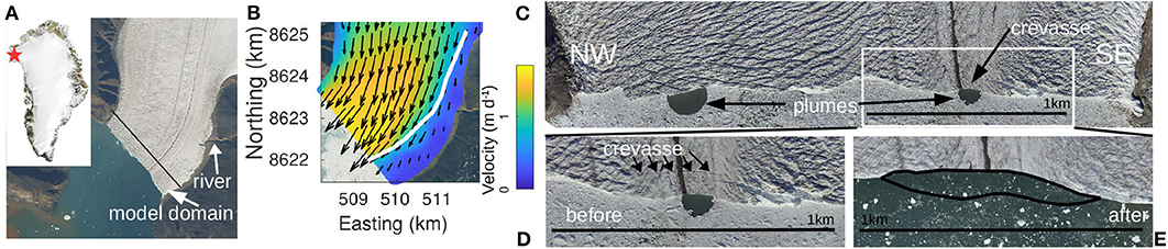
Figure 1. Satellite image, ice surface velocity fields, and ortho-images of Bowdoin Glacier. (A) Sentinel-2A image of Bowdoin Glacier on 25 July 2017, with an inset indicating the position of Bowdoin Glacier in Greenland by a star (Source: MODIS). One arrow points at the model domain, of which the upstream boundary is outlined by the black line. The other arrow points at the river that transports discharge from the nearby Mirror Glacier. (B) Satellite-derived velocity for the period 4–24 July 2017, including the shearline in white that outlines highest velocity gradients (van Dongen et al., 2020). (C–E) UAV-derived ortho-images before (C,D, July 5) and after the July 8 major calving event (E, July 14). (C) Northwest and southeast are labeled with NW and SE, respectively. (D) Several arrows point at the crevasse that lead to calving. (E) The July 8 calving event is outlined in black.

2. Study Site

Bowdoin Glacier is a marine-terminating glacier located in Northwest Greenland (77°N, 68°W, Figure 1A). The approximately 3 km wide glacier was up to 250 m thick at the calving front in 2013 (Sugiyama et al., 2015). The terminus position was fairly stable from 1987 to 2008, when the glacier started retreating at an average rate of 0.22 km yr⁻¹ (Sugiyama et al., 2015). Since 2013, the calving front has stabilized, but the glacier has been thinning at a rate of 4 m yr⁻¹ (Tsutaki et al., 2016). Bowdoin Glacier's ice flow is characterized by a stagnant region in the southeast and fast flow in the central region, causing a shear zone at the terminus (outlined in Figure 1B). An almost crevasse-free medial moraine is present ~1 km away from the southeastern glacier margin, close to the zone of highest shear (Figures 1B,C).

In July 2017, the break off of a 650 m wide, 80 m long iceberg was observed in detail during a field campaign, at least 5 days after the formation of a large surface crevasse (van Dongen et al., 2020). The fracture leading to the major calving event was the only crevasse that crossed both the shear zone and moraine (Figure 1D). A very similar scale event, at the same location across the shear zone, took place in July 2015, 15 days after fracture initiation (Jouvet et al., 2017). For both observed events, a plume was visible on the sea surface at the calving location (Figure 1C, Jouvet et al., 2017). Therefore, submarine melt-induced, local undercutting may have influenced the stress-state and thereby the observed calving events. In 2017, a second plume surfaced through the ice mélange in the northwest (Figure 1C). Jouvet et al. (2018) found that in 2016, the northwestern plume originated from Bowdoin Glacier itself, whereas the southeastern plume was fed by discharge from the nearby land-terminating Mirror Glacier. The plume's origin was recognized since it appeared approximately 24 h after the outburst of an ice-dammed, marginal lake fed by a river transporting meltwater from Mirror Glacier (Figure 1A).

3. Methods

3.1. Crevasse Detection

To facilitate the comparison of model results and observations, fractures are extracted from a 0.5 m resolution UAV-derived ortho-image of 5 July 2017 (Figure 1C). Various edge detection algorithms have been tested, but a simple threshold on intensity of the gray-scale ortho-image was the most successful in producing a crevasse map while limiting extraction of false positives (shadows, debris on the glacier etc.). Fractures are extracted by selecting the pixels with intensity below 30% from the ortho-image.

3.2. Model

We use the Helsinki Discrete Element Model (HiDEM, Åström et al., 2013, 2014) to study crevasse initiation prior to the observed large calving in 2017. HiDEM models ice as a brittle-elastic solid. Dynamics is induced by elasticity, fracture, and sliding. The model neglects viscous deformation, which can be ignored during fracture initiation and calving due to the distinct deformation timescales involved (~10²−10⁶ s for viscous deformation compared to ~10⁻² s for crack propagation, Benn et al., 2017).

HiDEM represents ice as an assemblage of particles, arranged to form glacier geometries. Neighboring particles are connected by massless breakable beams, that act as rigid joints keeping particles together. Regardless of whether two particles are connected by a beam, they interact via inelastic contacts that dissipate energy through a damping force. The version of HiDEM used in this study (doi: 10.5281/zenodo.1402603) most closely resembles the one described in Åström et al. (2014). A detailed model description is given in the Supplementary Material. Extensive benchmarking and validation of the model are reported in Riikilá et al. (2015) and Åström et al. (2013).

HiDEM computes the displacement of each particle using a discrete version of Newton's equation of motion with dissipation terms (Equation S1). Calculating the trajectory of each particle is computationally expensive, which restricts the duration of HiDEM simulations. During initial simulations, it became clear that the short timescale of our HiDEM runs (5 s) are sufficient for fractures to occur, but insufficient for sliding. Without glacier dynamics by sliding, only very limited fracture initiation occurs. To be able to simulate at least moderate sliding, the friction parameter (C in Equation S1) was rescaled by a factor of 10⁻⁵. With this rescaled friction coefficient, a few seconds of HiDEM simulation reproduces an amount of glacier sliding and fracturing that would normally require tens of hours. Only basal friction is scaled; all other forces such as gravity and particle interactions remain unscaled.

To start a simulation, the glacier is divided into a hexagonal close packed lattice of spheres of equal size. Initially, 10% of the beams are randomly selected and broken, representing small pre-existing cracks in the ice. Because the initial arrangement of particles is an undeformed lattice, there is no load on the beams to counter the forces induced by gravity and buoyancy. Therefore, the initially imposed lattice must deform slightly to reach a force-equilibrium before fracture initiation can be modeled. We first switch on the dynamics, including sliding but without fracture, and let the glacier deform under its own weight. The settling of particles toward force-equilibrium initially causes some internal oscillations that must be damped out before the model ice can be allowed to break. After 10 s of simulation, the kinetic energy of the glacier (Equation S3), mainly induced by these oscillations, is reduced by more than an order of magnitude (Figure S1). The mean particle displacement in this phase is less than 10cm in the horizontal direction and less than the particle size in the vertical direction (<2 m). Once the system has reached force-equilibrium, the load on beams can be expected to model forces within the glacier in a realistic manner. This is a suitable initial state for fracture computations and fracturing is allowed to occur in the second phase. Beams can break if the strain on a beam exceeds a fracture threshold, either by tension or bending (Equation S2). Fractures are irreversible, there is no reconnecting of beams. If all beams would break, the particle motion represents granular flow.

It should be noted that not all observed crevasses are formed instantaneously, many crevasses formed earlier and were advected to the terminus. Mottram and Benn (2009) measured strain rates across crevasses on a glacier in Iceland and found that almost half of the tested crevasses (19 out of 44) were closing due to compressive stress. Since relict crevasses may no longer be in equilibrium with prevailing stresses, it is expected that HiDEM does not reproduce such fractures. However, the one crevasse that was observed to lead to calving was located in the shear zone, which is normally crevasse free (Figures 1C–E). This crevasse was therefore very likely formed in place, similar to observations in 2015 (Jouvet et al., 2017), and is thus suitable to study by HiDEM simulations.

3.3. Model Domain

The computational domain extends to 500 m upstream of the calving front (Figure 1A). We use a highly detailed, 1 m resolution, Digital Surface Model (DSM) of 5 July 2017 obtained by UAV photogrammetry and bed elevation is derived from radar and sonar measurements (van Dongen et al., 2020). Glacier thickness in the model domain is shown in Figure 2B. The glacier front is grounded but close to flotation (van Dongen et al., 2020). Since we use a high resolution DSM, topographic depressions are present in the initial geometry. Figure 2C shows these depressions, calculated as the difference of the DSM and a smoothed surface obtained from the DSM by a 2-D median filter with a 51 × 51 kernel. We find that the topographic depressions do not affect the location and orientation of modeled fractures significantly, compared with a simulation imposing the smoothed surface (section 2.2 of Supplementary Material).

FIGURE 2

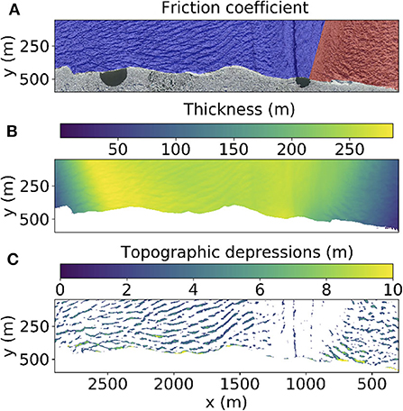
Figure 2. HiDEM input data on a rotated coordinate system, equal to the coordinate system of the HiDEM simulations. (A) Friction distribution overlayed on July 5 ortho-image, showing low friction (blue, 3 × 10⁹ kg s⁻¹) and high friction (red, 1 × 10¹¹ kg s⁻¹). (B) Glacier thickness and (C) topographic depressions, calculated as the difference of the DSM and a smoothed surface obtained from the DSM by a 2-D median filter with a 51 × 51 kernel.

Figure 3 shows the HiDEM domain after the relaxation phase, for a particle size of 1.75 m using ~50 million particles. A sensitivity analysis was done to find the optimal particle size, defined as particle diameter, that is computationally feasible and realistically reproduces fracturing on Bowdoin Glacier (section 2.1 of Supplementary Material). For large particles (≥4 m), hardly any fractures initiate. For small particles (≤2 m), the glacier becomes fragile and fracture initiation dominates the modeled velocity. Therefore, we use 2.5 m particles such that the model reproduces both fracture initiation and observed velocities.

FIGURE 3

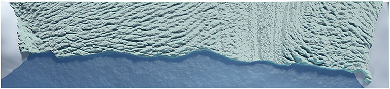
Figure 3. Particle arrangement describing the geometry of Bowdoin Glacier after 10 s of simulated glacier dynamics for a particle size of 1.75 m.

3.4. Boundary Conditions

Particles at the upstream and lateral boundaries are fixed in the horizontal plane. Unless specified otherwise, the glacier front is assumed to be vertical. A buoyancy force is applied to all ice particles below sea level, not only the particles at the calving front. This is equivalent to applying a water pressure at the calving front, the floating ice base and inside crevasses (as explained in the Supplementary Material).

Basal friction is applied as damping force, which is linearly related to particle velocity (Equation S1). We apply a simple friction distribution, based on satellite-derived velocity. A shear line is identified where the highest velocity gradients are observed (Figure 1B). Two different friction values are applied on either side of the shear line: a low friction of 3 × 10⁹ kg s⁻¹ and high friction of 1 × 10¹¹ kg s⁻¹ (Figure 2A). The values are averaged friction values found by inverting for basal friction based on the satellite-derived velocity using the ice flow model Elmer/Ice (van Dongen et al., 2020). The values of all model parameters are listed in Table S1.

3.5. Experiment Design

We define a control simulation, which has the dual basal friction distribution shown in Figure 2A and a vertical ice cliff. Besides the control simulation, we test the influence of the basal conditions and undercutting.

Usually, no fractures are present in the shear zone (Figures 1B,C), similar to observed at Antarctic suture zones (e.g., Hulbe et al., 2010). However, the fractures leading to the major calving events in 2015 and 2017 did cross the shear zone. Therefore, it has been argued that influence of the shear zone on fracture formation is important to understanding the observed calving event (Jouvet et al., 2017; van Dongen et al., 2020). To assess the influence of the observed high shear, we compare our control simulation to a set-up with the low friction value everywhere.

Since a plume surfaced at the calving location, we expect that local undercutting influenced the major calving event. Therefore, several experiments are conducted with a submarine melt-induced undercut. As there has not been in-situ measurement of the shape of the submarine ice-cliff at Bowdoin Glacier, we have to assume ice front geometries based on observations at other glaciers (Fried et al., 2015; Rignot et al., 2015; How et al., 2019). We assume linear undercuts reaching up to sea level, similar to those used by Benn et al. (2017). We vary the undercut length (UC), which is defined as the distance upstream the undercut reaches. We let the undercut length depend on the local water depth (D_w, Figure 4). Three different types of undercuts are introduced: a distributed undercut along the entire calving front, local undercuts where plumes are observed through the ice mélange (Figure 1C) or a combination of a smaller distributed and larger local undercut. An overview of the simulations is given in Table 1 and the undercut geometries are outlined in red on Figures 6B–E.

FIGURE 4

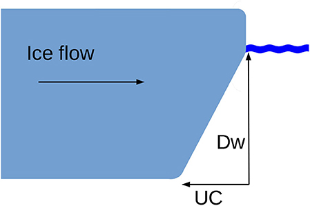
Figure 4. Conceptual visualization of the undercut geometry, showing definition of undercut length UC, and water depth D_w. Here UC = D_w/2.

TABLE 1

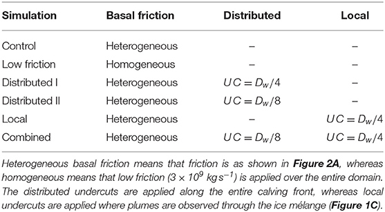
Table 1. Summary of numerical experiments.

The maximum applied distributed undercut in our simulations is D_w/4. Observed undercut lengths averaged across a terminus, hence similar to our distributed undercut, vary from D_w/10−D_w/3 for Greenlandic glaciers (Fried et al., 2015; Rignot et al., 2015). The reported largest local undercut lengths vary widely per glacier as well: from D_w/12 for Tunabreen (Svalbard), D_w/2 for Kangilernata Sermia to D_w for Kangerlussuup Sermia, Store Gletscher, and Rink Isbrae (Fried et al., 2015; Rignot et al., 2015; How et al., 2019). Because of high computational demands, the number of experiments is severely limited and not the entire range of observed local undercuts has been simulated.

4. Results

4.1. Observed Crevasse Distribution

Detected crevasses are shown in Figure 5A. Besides crevasses, a few dark features are also extracted, such as the medial moraine and some patches with debris close to the moraine, but the criterion is chosen such that shadows are not extracted. Figure 5A shows four regions of different fracturing patterns. Long, transverse crevasses are observed in the fast flowing area (1250 ≤ x ≤ 2500 m). Close to the western glacier margin (x > 2500 m), narrow along-flow crevasses are visible besides wider across-flow crevasses. Except for the crevasse leading to calving (Figures 1C–E), very few crevasses are observed in the shear zone close to the moraine (850 ≤ x ≤ 1250 m). Close to the eastern margin (x ≤ 850 m), crevasse density increases again but the fracturing pattern is more chaotic than in other regions of the glacier terminus. Since only minor sliding is expected in this area (Figure 1B, Jouvet et al., 2017), these crevasses are presumably produced under a dynamical regime of slow stretching mostly due to viscous deformation.

FIGURE 5

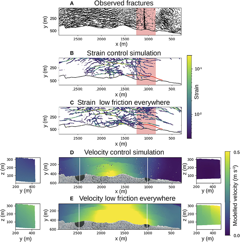
Figure 5. Comparison of observed and modeled fractures for the control and low friction set-up. (A) Observed fractures extracted by selecting the pixels with intensity below 30% of the maximum intensity, from the 0.5 m resolution ortho-image of July 5 (Figure 1C). (B) Modeled fractures above sea level with strain larger than 0.003 (10 times the fracture strain) for the control simulation, after 15 s simulation. (C) Modeled fractures when applying low friction everywhere. (A–C) The red area highlights the shear zone (850 ≤ x ≤ 1250). (B,C) The red line indicates the extent of the observed calving event. Modeled velocity from 10 to 15 s simulation time for (D) the control simulation and (E) low friction everywhere. (D,E) Left panels show a cross-section through the northwestern plume, middle panels surface velocity and right panels a cross-section through the southeastern plume. The white lines in the middle panels indicate the location of the cross-sections.

The same four regions (western marginal, central, shear zone and eastern marginal) will also be referred to in comparisons of model results versus observed fracturing pattern. We have computed the density of black pixels in Figure 5A per region, as a measure of observed crevasse density (both abundance and width), as shown in Table 2. For the calculation of crevasse density in the shear zone, the moraine-covered area (1050 ≤ x ≤ 1100 m) is excluded since the gray-scale threshold falsely detects it as a crevasse. The crevasse densities in Table 2 for each region are given relative to the density in the entire domain. Table 2 shows that the observed crevasse density is highest in the western marginal area, closely followed by the central area. The observed crevasse density is lowest in the shear zone.

TABLE 2

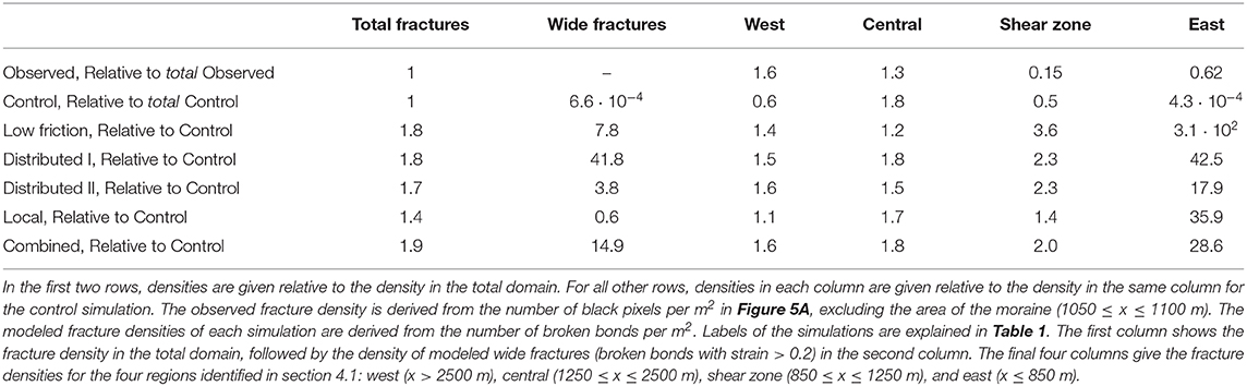
Table 2. Fracture densities as observed (first row) and modeled (all other rows).

In sections 4.2 and 4.3 we assess whether HiDEM reproduces the observed crevasse pattern. Subsequently, section 4.4 addresses the influence of undercut geometries on the initiation of the crevasse that was observed to lead to major calving (Figures 1C–E), and other crevasses close to the front that could induce calving.

4.2. Control Simulation

All simulations are run for 5 s in the second simulation phase when fracturing is allowed. The 5 s of modeled glacier dynamics resemble the amount of sliding that is observed in approximately one day (Figure 5D). This is as expected, since the basal friction coefficient is scaled by a factor 10⁻⁵, and the sliding velocity is approximately proportional to friction coefficient (Equation S1). As such, we can interpret the modeled fractures to represent the amount of fractures that initiate during approximately one day. HiDEM reproduces the observed high shear close to the moraine (Figure 5D). The velocity distribution is partly characterized by fracture initiation, visible as discontinuities in the modeled velocity field (Figure 5D).

Modeled fracture strain on the surface is shown in Figure 5B. The strain is only shown for broken bonds where the strain is at least ten times the fracture strain. Strain magnitude reflects fracture width: if the strain is 1, this corresponds to a fracture width equal the original bond length which is slightly larger than the particle size (2.8 m). Generally, modeled fracture orientation agrees with observations, but the modeled fracture density is much lower than observed. Fractures are mainly initiated in the central area (Table 2), which matches the area where the long, transverse fractures are observed (Figure 5A). However, the fractures do not extend as far to the west as observed. This results in a low modeled fracture density in the western marginal area, which contradicts observations (Table 2). Very few crevasses are modeled in the shear zone, which is consistent with observations, and the few crevasses modeled there are narrow (low strain in Figure 5B). One of the modeled fractures is similar to the crevasse that lead to the observed calving event, only along half of its extent. In the almost stagnant eastern marginal area, a very low fracture density is modeled, contrary to observations, but this should be expected because our model set-up ignores viscous deformation (see section 4.1 and 5).

4.3. Basal Conditions

The low friction set-up causes significantly more fractures (Figure 5C): the proportion of broken bonds is almost twice as high as in the control set-up (Table 2). By lowering the friction in the eastern marginal area, the ice velocity is generally higher than in the control simulation (cf Figures 5D,E). Hence, the increased glacier sliding causes increased fracture initiation. At first sight, the low friction set-up therefore does a better job in reproducing the observed fractures than the control simulation, which showed a lower fracture density. Especially in both marginal areas, more fractures are modeled in comparison to the control simulation (Table 2). However, we do not expect our model set-up to reproduce crevasses in the eastern marginal area. Therefore, we do not interpret the higher modeled fracture density in the east as an improvement compared with the control simulation. Furthermore, the low friction set-up no longer reproduces the almost stagnant area in the east. Almost four times as many fractures initiate in the low friction set-up in the shear zone (Table 2), where very few fractures are observed. The shear zone is of main interest in this study, since calving was observed there. Because the control simulation better reproduces the shear zone, all subsequent simulations assume the friction distribution as in the control simulation (Figure 2A), despite the better reproduction of the western marginal area in the low friction set-up.

4.4. Melt-Induced Undercutting

Four different undercut geometries are applied (see Table 1). Moderate (UC = D_w/8) or larger (UC = D_w/4) distributed undercuts are applied along the entire calving front, as well as a local undercut (UC = D_w/4, Figure 4). Finally, a local undercut (D_w/4) at the plumes which gradually decreases to a moderate distributed undercut (D_w/8) everywhere else is applied. For all simulations, the surface strain is shown in Figures 6B–E and modeled velocity averaged from 14 to 15 s in Figures 6G–J. For comparison, strain and velocity of the control simulation are shown in Figures 6A,F. As can be seen from comparing Figure 5D (10–15 s velocity average for the control simulation) and Figure 6F (14–15 s velocity average for the same simulation), the 10–15 s averaged velocity is dominated by smooth sliding, whereas the velocity from 14 to 15 s is dominated by discrete fracturing. Since we are mainly interested in the fracturing for these undercut simulations, the velocity during the final second of simulation is shown, such that the fractures that are actively opening are visualized. The quantity of modeled broken bonds, wide crevasses and crevasses in the shear zone, relative to the control simulation, are given in Table 2.

FIGURE 6

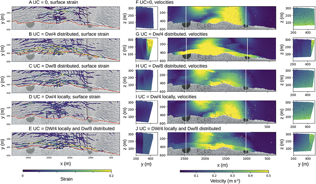
Figure 6. Comparison of modeled fractures for the undercut experiments. (A–E) All bonds above sea level with fracture strain over 0.01 after 15 s are shown for several undercut geometries (B–E), compared with the control set-up (A), overlayed on the ortho-image of July 5. (A–E) White lines indicate the extent of the observed calving event and red lines the applied undercut length for each simulation. (F–J) Modeled velocity from 14 to 15 s simulation time for the same geometries, where left panels show a cross-section through the northwestern plume, middle figures surface velocity, and right figures a cross-section through the southeastern plume. The white lines through the middle panels indicate the location of the cross-sections.

The model results suggest that the larger distributed undercut (UC = D_w/4) destabilizes the entire glacier terminus. Figure 6B not only shows more surface fractures but also higher strain, hence wider fractures (more than forty times as many wide fractures, Table 2). The velocity cross-sections furthermore show that fractures extend to the ice base and ice chunks are in the process of rapidly detaching up to 200 m upstream, across the whole terminus (Figure 6G). As such, the modeled fractures can be interpreted as a precursor to a very large calving event which spans almost the whole glacier width. On the other hand, the moderate distributed undercut has a very limited effect on fracture initiation (Figure 6C, four times as many wide fractures, Table 2) and velocity (Figure 6H). Only in the western marginal area, a few fractures are initiated where no fractures were modeled in the control simulation (Figure 6A), but the fracture density in the west is still lower than observed.

The modeled surface strain shows that a local undercut (Figure 6D) does not affect fracture initiation much. Fracturing is still limited in the west and the quantity of modeled fractures is very similar to the control set-up (Table 2). However, the combined effect of a local larger undercut, gradually decreasing to a distributed moderate undercut, produces wider fractures than either the local or distributed moderate undercut (Figure 6E). The total increase of fractures is slightly larger than for the distributed D_w/4 undercut, but fewer wide crevasses are modeled (less than half the increase, Table 2). The wider fractures do not extend as far upstream the calving front as for the larger distributed undercut (cf. extent of yellow in Figures 6B,E) and fractures are opening less rapidly (cf. Figures 6G,J). For the combined local and distributed undercut, one wide fracture outlines the observed fracture that lead to calving (Figure 6E). The velocity cross-sections show that a fracture extends to the glacier base near the northwestern plume and the ice chunk near the southeastern plume that was observed to calve off is detaching (Figure 6J).

The model results of the combined local and moderate distributed undercut are compared with observations in Figure 7. The observed and modeled velocity show a similar discontinuity where calving is observed (Figures 7A,B), although the velocity distributions do not agree. Whereas the iceberg is observed to have the highest detachment velocity on the southeast, the modeled velocity is lower there. Figure 7C shows that the modeled fracture does not exactly follow the applied undercut length, but is initiated further upstream, close to where calving is observed (Figure 7D). Both the distributed D_w/4 undercut and combined local and distributed undercuts results show a major crevasse in close alignment with the crevasse that was observed to lead to major calving. In order to quantify the difference between the modeled and observed crevasse for both simulations, we calculated the area between the closest modeled crevasse and the observed crevasse. We divided this area by the observed crevasse length to get the average distance between the modeled and observed crevasse. For the distributed UC = D_w/4, the closest crevasse is on average 15.3 m away from observations, whereas the combined local and distributed undercuts give a crevasse on average 6.5 m close to observed, less than three times the particle size.

FIGURE 7

Figure 7. Comparison of model results and observations for UC = D_w/4 locally, decreasing to D_w/8 distributed. (A) TRI-derived velocity averaged from 5 July until the calving event on 8 July (van Dongen et al., 2020), (B) modeled velocity, (C) modeled strain, with a red line showing the extent of the applied undercut, and (D) an ortho-image after calving, with a white line showing the previous calving front position.

5. Discussion

In an earlier study (van Dongen et al., 2020), the relative importance of several physical processes that could affect crevasse opening was investigated by comparing ice flow model results to observations. Crevasse water level and thus hydro-fracturing was found to be a first-order control on opening rates. Submarine melt-undercutting was identified as a second-order process, possibly accelerating opening rates. However, the previous study only addressed opening of the crevasse leading to calving, after it had initiated. Here, we investigate fracture initiation, using the elastic-brittle model HiDEM. The simulations serve to increase our understanding of the calving pattern observed at Bowdoin Glacier and to assess the effect of melt-undercutting.

The high-shear zone in the southeast, close to the medial moraine (Figure 1B), has been suggested to influence the calving pattern of Bowdoin Glacier (Jouvet et al., 2017). HiDEM produces high shear when using a dual basal friction distribution with higher friction in the slow-flowing area (Figure 5D). The almost crevasse-free area in the shear zone is in this case well reproduced (Figure 5B). On the other hand, if applying low friction everywhere, the fracture density increases by a factor of almost four in the shear zone (Table 2). These results support the suggested importance of basal conditions to explain the observed fracturing pattern in the shear zone.

Besides geometry and basal friction, the only model input consisted of conceptual ice-cliff profiles, based on locations of plumes at Bowdoin Glacier and measured ice-cliff profiles at other glaciers (Fried et al., 2015; Rignot et al., 2015; How et al., 2019). Due to high computational demands, only a small set of geometries could be tested. We demonstrate that HiDEM nevertheless manages to closely reproduce the fracture initiation prior to the observed large calving of 8 July 2017, on average 6.5 m close to observed, as shown in Figure 7.

The HiDEM results suggest that the modeled fracture initiation and thus the calving behavior are strongly controlled by submarine melt-induced undercuts (Figure 6). When applying a large distributed undercut (UC = D_w/4 along the entire calving front), HiDEM predicts collapse of almost the entire width of the ice cliff (Figure 6G). As such collapse is not observed, we interpret the applied undercut to be unrealistically large, since the simulation suggests that calving would have occurred before the undercut could grow this large. The impact on fracturing is limited when applying a moderate distributed undercut (UC = D_w/8) or local undercuts restricted to plumes (UC = D_w/4, Figures 6C,D,H,I). However, HiDEM reproduces the observed fracture that lead to calving very closely when the moderate distributed undercut is combined with larger local undercuts (Figures 6E,J, 7), although we cannot exclude that other combinations of local and distributed undercuts not tested here could have produced a similar result. The simulation combining a moderate distributed and larger local undercuts also shows fractures near the western plume that could lead to calving (Figure 6E). However, these fractures are narrower and do not extend all the way to the front, which suggests that they would not lead to detachment of an iceberg yet (Figure 6E). Sentinel-2 imagery confirms that calving occurred in this region between July 30 and August 19.

The assumed undercut lengths are in the range of observed undercuts for West Greenlandic glaciers, where the majority of the calving front is undercut (range of distributed UC from D_w/10 to D_w/3) and plumes cause local deeper undercuts (up to D_w, Fried et al., 2015; Rignot et al., 2015). The occurrence of a calving amplifier (O'Leary and Christoffersen, 2013) can be examined by comparing the upstream extent of the applied undercuts to the modeled initiation of wider fractures (strain>0.2, yellow in Figures 6B–E). In our simulations, increased fracturing is limited in case of a moderate distributed undercut (D_w/8) or larger local undercuts (D_w/4, Figures 6C,D). With a larger distributed undercut, wider fractures are initiated over 200 m upstream in the central part of the terminus, more than four times further than the undercut itself (D_w/4, Figure 6B). Besides that, the combination of a larger local and a moderate distributed undercut increases fracture initiation over 100 m upstream, both at and in between the local undercuts (Figure 6E). Hence, our results exhibit the calving amplifier effect both upglacier (as in O'Leary and Christoffersen, 2013) and across-glacier (as in Cowton et al., 2019). However, the calving amplifier does not appear in our simulations for local undercuts alone (cf. Figures 6A,D). This is in line with Todd et al. (2018), who used a crevasse-depth calving model to show that distributed undercutting most strongly affects retreat (cf. Figures 6A,B), whereas concentrated melting generally has little influence on fracturing (cf. Figures 6A,D), unless a plume is situated at a “key stone,” where stress bridges provide lateral support to the ice front.

The findings of our highly detailed simulations agree with previous HiDEM studies, which showed that undercutting is necessary to explain satellite-derived mean volumetric calving rates for Kronebreen (Svalbard, Vallot et al., 2018) and that sufficiently large undercuts may induce calving lengths of several times the undercut length for conceptual glacier geometries (Benn et al., 2017). Whether an undercut can grow large enough to act as an amplifier may depend on the frequency of low-magnitude calving events (Benn et al., 2017). If small calving events are rare and an undercut is able to grow, instability builds up and the terminus may approach a critical state which increases the probability of large calving events. This process can also be described by self-organized criticality (SOC, Åström et al., 2014). SOC systems have a sub-critical regime—in this case distinguished by infrequent and small calving events, allowing an instability to build up with time—and a super-critical regime—distinguished by large calvings and widespread relaxation of the instability. Our simulations with small or no undercut show typical sub-critical behavior, characteristic of quiescent periods of calving. In contrast, the larger distributed undercut shows super-critical collapse of the entire calving front, which is unlikely to happen in nature. This explains the behavior of Bowdoin Glacier which shows infrequent large calving events—such as observed in recent years (Jouvet et al., 2017; Minowa et al., 2019)—that relax its terminus back to sub-criticality and let undercuts grow again by submarine melting, destabilizing the front, yielding a cyclic calving pattern.

Our results thus confirm a complex interaction of a distributed melt-undercut along the entire ice cliff, and enhanced melt-undercutting at the locations of plumes. Similar detailed observational and modeling studies are required on more glaciers to quantify the links between melt-undercutting and calving at tidewater glaciers such as Bowdoin.

A major limitation of our modeling approach is the short simulation duration (a few seconds, corresponding to approximately one day of sliding), which does not permit modeling of the entire calving event from fracture initiation to detachment of the iceberg (at least five days according to observations).

A shortcoming of our control simulation is the relatively low modeled fracture density in the western marginal area, both compared with the low friction set-up and with observations. Most likely, the higher modeled fracture density can be explained by the modeled ice velocity, which is not only lower in the eastern marginal area compared with the low friction simulation, but across the terminus (Figure 5E). Comparison of modeled and observed velocity shows that the velocity is underestimated in the western marginal area for both the control and low friction set-up. Whereas the area of high velocity is observed to extend to the western margin, modeled velocities in the west are lower than in the central area, which can presumably explain the low modeled fracture density in the west (compare Figures 5D,E, 1B).

Furthermore, the modeled density of surface fractures is generally lower than observed (Figure 5A), which can have two causes. First, fracture simulations lack history, whereas part of the observed crevasses are formed upstream and advected to the terminus. Future work could employ more detailed observations to distinguish actively opening crevasses from relict crevasses which are not in equilibrium with prevailing stresses. This would allow a more quantitative comparison of observations of active crevasses and modeled fracture initiation, whereas our comparisons remain rather qualitative.

Second, viscous deformation is not included in the simulations. The force imbalance at the ice-cliff is key to understanding the emergence of surface crevasses at a glacier terminus. Because the outward-directed cryostatic pressure is greater than the inward-directed hydrostatic pressure, viscous stretching is required to balance the gradient in longitudinal stress (Benn et al., 2007). Consequently, viscous stretching will increase tensile fracture at the glacier surface. This is especially the case in the almost stagnant eastern marginal area, where only minor sliding is expected, and fractures are presumably mainly induced by viscous stretching. Employing a viscoelastic rheology for ice would therefore improve modeling work of this kind.

6. Conclusions

This study investigated the calving mechanisms of Bowdoin Glacier, Northwest Greenland. A major calving event from summer 2017 was studied, by comparing numerical calving model simulations with observations. Using the Helsinki Discrete Element Model (HiDEM), we modeled fracture initiation prior to the calving event. The HiDEM results show that the fracturing pattern is strongly controlled by basal conditions and undercuts induced by submarine melt. The almost stagnant area on the eastern glacier margin creates a shear zone in which very few fractures initiate. On the other hand, we find that submarine melt-induced undercutting may amplify calving. Experiments with various undercut geometries show that the modeled increase in fracture initiation generally reaches further upstream than the applied undercut. However, the interaction between the undercut geometries and fracture initiation is complex. Local undercuts at the plumes alone do not increase fracturing, whereas combination with a smaller distributed, front-wide undercut leads to wider fractures across the terminus, both at and in between the plumes. Therefore, it is complicated, if not impossible, to quantify the modeled interaction between undercutting and fracturing towards a parameterized calving law. Nonetheless, our results show the importance of submarine melt-induced undercutting for calving behavior at grounded tidewater glaciers such as Bowdoin and motivate further detailed studies on this topic.

Data Availability Statement

The input files for HiDEM (geometry and simulation parameters) are available at https://doi.org/10.5281/zenodo.3872912.

Author Contributions

ED and GJ designed the study. ED carried out the numerical simulations and prepared the figures with support from JÅ, JT, and DB. MF organized the fieldwork at Bowdoin Glacier. ED drafted the manuscript with support from GJ and JÅ. All authors contributed to the final version.

Funding

This research was part of the Sun2ice project (ETH Grant ETH-12 16-2), supported by the Dr. Alfred and Flora Spälti and the ETH Zurich Foundation. Fieldwork was funded by the Swiss National Science Foundation, grant 200021-153179/1. The HiDEM simulations were performed under the Project HPC-EUROPA3 (INFRAIA-2016-1-730897), with the support of the EC Research Innovation Action under the H2020 Programme; in particular, the authors gratefully acknowledge the computer resources and technical support provided by CSC-IT Centre for Science in Finland. DB and JT were funded by NERC grant NE/P011365/1 (CALISMO: Calving Laws for Ice Sheet Models).

Conflict of Interest

The authors declare that the research was conducted in the absence of any commercial or financial relationships that could be construed as a potential conflict of interest.

Acknowledgments

We thank the members of the 2017 field campaign on Bowdoin Glacier and in particular Shin Sugiyama for co-organizing the expedition and Andrea Walter for collecting and processing the TRI data and operating the UAV. We thank Fabian Walter for valuable discussions and supervision. We acknowledge Julien Seguinot for providing Sentinel-2A satellite images processed with Sentinelflow (Seguinot, 2018). The simulated graphics in Figure 3 have been rendered by Jyrki Hokkanen (CSC-IT Centre for Science). The authors thank the editor and the referees for their constructive comments, which contributed to improve the manuscript.

Supplementary Material

The Supplementary Material for this article can be found online at: https://www.frontiersin.org/articles/10.3389/feart.2020.00253/full#supplementary-material

References

Åström, J. A., Riikilá, T. I., Tallinen, T., Zwinger, T., Benn, D., Moore, J. C., et al. (2013). A particle based simulation model for glacier dynamics. Cryosphere 7, 1591–1602. doi: 10.5194/tc-7-1591-2013

CrossRef Full Text | Google Scholar

Åström, J. A., Vallot, D., Schäfer, M., Welty, E. Z., O'Neel, S., Bartholomaus, T. C., et al. (2014). Termini of calving glaciers as self-organized critical systems. Nat. Geosci. 7, 874–878. doi: 10.1038/ngeo2290

CrossRef Full Text | Google Scholar

Bassis, J., and Jacobs, S. (2013). Diverse calving patterns linked to glacier geometry. Nat. Geosci. 6:833. doi: 10.1038/ngeo1887

CrossRef Full Text | Google Scholar

Benn, D. I., Åström, J., Zwinger, T., Todd, J., Nick, F. M., Cook, S., et al. (2017). Melt-under-cutting and buoyancy-driven calving from tidewater glaciers: new insights from discrete element and continuum model simulations. J. Glaciol. 63, 691–702. doi: 10.1017/jog.2017.41

CrossRef Full Text | Google Scholar

Benn, D. I., and Åström, J. A. (2018). Calving glaciers and ice shelves. Adv. Phys. X 3:1513819. doi: 10.1080/23746149.2018.1513819

CrossRef Full Text | Google Scholar

Benn, D. I., Warren, C. R., and Mottram, R. H. (2007). Calving processes and the dynamics of calving glaciers. Earth Sci. Rev. 82, 143–179. doi: 10.1016/j.earscirev.2007.02.002

CrossRef Full Text | Google Scholar

Bulthuis, K., Arnst, M., Sun, S., and Pattyn, F. (2019). Uncertainty quantification of the multi-centennial response of the antarctic ice sheet to climate change. Cryosphere 13, 1349–1380. doi: 10.5194/tc-13-1349-2019

CrossRef Full Text | Google Scholar

Carroll, D., Sutherland, D. A., Hudson, B., Moon, T., Catania, G. A., Shroyer, E. L., et al. (2016). The impact of glacier geometry on meltwater plume structure and submarine melt in Greenland fjords. Geophys. Res. Lett. 43, 9739–9748. doi: 10.1002/2016GL070170

CrossRef Full Text | Google Scholar

Catania, G., Stearns, L., Moon, T., Enderlin, E., and Jackson, R. (2019). Future evolution of Greenland's marine-terminating outlet glaciers. J. Geophys. Res.: Earth Surface 125:e2018JF004873. doi: 10.1029/2018JF004873

CrossRef Full Text | Google Scholar

Colgan, W., Rajaram, H., Abdalati, W., McCutchan, C., Mottram, R., Moussavi, M. S., et al. (2016). Glacier crevasses: observations, models, and mass balance implications. Rev. Geophys. 54, 119–161. doi: 10.1002/2015RG000504

CrossRef Full Text | Google Scholar

Cowton, T., Slater, D., Sole, A., Goldberg, D., and Nienow, P. (2015). Modeling the impact of glacial runoff on fjord circulation and submarine melt rate using a new subgrid-scale parameterization for glacial plumes. J. Geophys. Res. Oceans 120, 796–812. doi: 10.1002/2014JC010324

CrossRef Full Text | Google Scholar

Cowton, T. R., Todd, J. A., and Benn, D. I. (2019). Sensitivity of tidewater glaciers to submarine melting governed by plume locations. Geophys. Res. Lett. 46, 11219–11227. doi: 10.1029/2019GL084215

CrossRef Full Text | Google Scholar

Faillettaz, J., Sornette, D., and Funk, M. (2011). Numerical modeling of a gravity-driven instability of a cold hanging glacier: reanalysis of the 1895 break-off of Altelsgletscher, Switzerland. J. Glaciol. 57, 817–831. doi: 10.3189/002214311798043852

CrossRef Full Text | Google Scholar

Fried, M. J., Catania, G. A., Bartholomaus, T. C., Duncan, D., Davis, M., Stearns, L. A., et al. (2015). Distributed subglacial discharge drives significant submarine melt at a Greenland tidewater glacier. Geophys. Res. Lett. 42, 9328–9336. doi: 10.1002/2015GL065806

PubMed Abstract | CrossRef Full Text | Google Scholar

Gagliardini, O., Zwinger, T., Gillet-Chaulet, F., Durand, G., Favier, L., Fleurian, B. D., et al. (2013). Capabilities and performance of Elmer/Ice, a new-generation ice sheet model. Geosci. Model Dev. 6, 1299–1318. doi: 10.5194/gmd-6-1299-2013

CrossRef Full Text | Google Scholar

Goelzer, H., Nowicki, S., Payne, A., Larour, E., Seroussi, H., Lipscomb, W. H., et al. (2020). The future sea-level contribution of the Greenland ice sheet: a multi-model ensemble study of ISMIP6. Cryosphere Discuss. 2020, 1–43. doi: 10.5194/tc-2019-319-supplement

CrossRef Full Text | Google Scholar

Hill, E. A., Carr, J. R., and Stokes, C. R. (2017). A review of recent changes in major marine-terminating outlet glaciers in northern Greenland. Front. Earth Sci. 4:111. doi: 10.3389/feart.2016.00111

CrossRef Full Text | Google Scholar

How, P., Schild, K., Benn, D., Noormets, R., Kirchner, N., Luckman, A., et al. (2019). Calving controlled by melt-under-cutting: detailed calving styles revealed through time-lapse observations. Ann. Glaciol. 60, 20–31. doi: 10.1017/aog.2018.28

CrossRef Full Text | Google Scholar

Hulbe, C. L., LeDoux, C., and Cruikshank, K. (2010). Propagation of long fractures in the Ronne Ice Shelf, Antarctica, investigated using a numerical model of fracture propagation. J. Glaciol. 56, 459–472. doi: 10.3189/002214310792447743

CrossRef Full Text | Google Scholar

IMBIE Team (2019). Mass balance of the Greenland Ice Sheet from 1992 to 2018. Nature 579, 233–239. doi: 10.1038/s41586-019-1855-2

PubMed Abstract | CrossRef Full Text | Google Scholar

Inall, M. E., Murray, T., Cottier, F. R., Scharrer, K., Boyd, T. J., Heywood, K. J., et al. (2014). Oceanic heat delivery via Kangerdlugssuaq Fjord to the south-east Greenland ice sheet. J. Geophys. Res. Oceans 119, 631–645. doi: 10.1002/2013JC009295

CrossRef Full Text | Google Scholar

Jackson, R., Nash, J., Kienholz, C., Sutherland, D., Amundson, J., Motyka, R., et al. (2020). Meltwater intrusions reveal mechanisms for rapid submarine melt at a tidewater glacier. Geophys. Res. Lett. 47:e2019GL085335. doi: 10.1029/2019GL085335

CrossRef Full Text | Google Scholar

Jenkins, A. (2011). Convection-driven melting near the grounding lines of ice shelves and tidewater glaciers. J. Phys. Oceanogr. 41, 2279–2294. doi: 10.1175/JPO-D-11-03.1

CrossRef Full Text | Google Scholar

Jouvet, G., Weidmann, Y., Kneib, M., Detert, M., Seguinot, J., Sakakibara, D., et al. (2018). Short-lived ice speed-up and plume water flow captured by a VTOL UAV give insights into subglacial hydrological system of Bowdoin Glacier. Remote Sens. Environ. 217, 389–399. doi: 10.1016/j.rse.2018.08.027

CrossRef Full Text | Google Scholar

Jouvet, G., Weidmann, Y., Seguinot, J., Funk, M., Abe, T., Sakakibara, D., et al. (2017). Initiation of a major calving event on the Bowdoin Glacier captured by UAV photogrammetry. Cryosphere 11, 911–921. doi: 10.5194/tc-11-911-2017

CrossRef Full Text | Google Scholar

Minowa, M., Podolskiy, E. A., Jouvet, G., Weidmann, Y., Sakakibara, D., Tsutaki, S., et al. (2019). Calving flux estimation from tsunami waves. Earth Planet. Sci. Lett. 515, 283–290. doi: 10.1016/j.epsl.2019.03.023

CrossRef Full Text | Google Scholar

Mottram, R. H., and Benn, D. I. (2009). Testing crevasse-depth models: a field study at Breidamerkurjökull, Iceland. J. Glaciol. 55, 746–752. doi: 10.3189/002214309789470905

CrossRef Full Text | Google Scholar

O'Leary, M., and Christoffersen, P. (2013). Calving on tidewater glaciers amplified by submarine frontal melting. Cryosphere 7, 119–128. doi: 10.5194/tc-7-119-2013

CrossRef Full Text | Google Scholar

Pritchard, H. D., Arthern, R. J., Vaughan, D. G., and Edwards, L. A. (2009). Extensive dynamic thinning on the margins of the greenland and antarctic ice sheets. Nature 461:971. doi: 10.1038/nature08471

PubMed Abstract | CrossRef Full Text | Google Scholar

Rignot, E., Fenty, I., Xu, Y., Cai, C., and Kemp, C. (2015). Undercutting of marine-terminating glaciers in West Greenland. Geophys. Res. Lett. 42, 5909–5917. doi: 10.1002/2015GL064236

PubMed Abstract | CrossRef Full Text | Google Scholar

Rignot, E., Koppes, M., and Velicogna, I. (2010). Rapid submarine melting of the calving faces of West Greenland glaciers. Nat. Geosci. 3:187. doi: 10.1038/ngeo765

CrossRef Full Text | Google Scholar

Riikilá, T., Tallinen, T., Åström, J., and Timonen, J. (2015). A discrete-element model for viscoelastic deformation and fracture of glacial ice. Comput. Phys. Commun. 195, 14–22. doi: 10.1016/j.cpc.2015.04.009

CrossRef Full Text | Google Scholar

Seguinot, J. (2018). Sentinelflow: automated satellite image workflow for Sentinel-2, v0.1.3. Zenodo. doi: 10.5281/zenodo.1774659

CrossRef Full Text | Google Scholar

Slater, D. A., Goldberg, D. N., Nienow, P. W., and Cowton, T. R. (2016). Scalings for submarine melting at tidewater glaciers from buoyant plume theory. J. Phys. Oceanogr. 46, 1839–1855. doi: 10.1175/JPO-D-15-0132.1

CrossRef Full Text | Google Scholar

Sugiyama, S., Sakakibara, D., Tsutaki, S., Maruyama, M., and Sawagaki, T. (2015). Glacier dynamics near the calving front of Bowdoin Glacier, northwestern Greenland. J. Glaciol. 61, 223–232. doi: 10.3189/2015JoG14J127

CrossRef Full Text | Google Scholar

Sutherland, D. A., and Straneo, F. (2012). Estimating ocean heat transports and submarine melt rates in Sermilik Fjord, Greenland, using lowered acoustic Doppler current profiler (LADCP) velocity profiles. Ann. Glaciol. 53, 50–58. doi: 10.3189/2012AoG60A050

CrossRef Full Text | Google Scholar

Todd, J., Christoffersen, P., Zwinger, T., Råback, P., Chauché, N., Benn, D., et al. (2018). A full-stokes 3-d calving model applied to a large greenlandic glacier. J. Geophys. Res. 123, 410–432. doi: 10.1002/2017JF004349

CrossRef Full Text | Google Scholar

Tsutaki, S., Sugiyama, S., Sakakibara, D., and Sawagaki, T. (2016). Surface elevation changes during 2007-13 on Bowdoin and Tugto Glaciers, northwestern Greenland. J. Glaciol. 62, 1083–1092. doi: 10.1017/jog.2016.106

CrossRef Full Text | Google Scholar

Vallot, D., Åström, J., Zwinger, T., Pettersson, R., Everett, A., Benn, D. I., et al. (2018). Effects of undercutting and sliding on calving: a global approach applied to Kronebreen, Svalbard. Cryosphere 12, 609–625. doi: 10.5194/tc-12-609-2018

CrossRef Full Text | Google Scholar

van Dongen, E., Jouvet, G., Walter, A., Todd, J., Zwinger, T., Asaji, I., et al. (2020). Tides modulate crevasse opening prior to a major calving event at Bowdoin Glacier, Northwest Greenland. J. Glaciol. 66, 113–123. doi: 10.1017/jog.2019.89

CrossRef Full Text | Google Scholar

Xu, Y., Rignot, E., Fenty, I., Menemenlis, D., and Flexas, M. M. (2013). Subaqueous melting of Store Glacier, west Greenland from three-dimensional, high-resolution numerical modeling and ocean observations. Geophys. Res. Lett. 40, 4648–4653. doi: 10.1002/grl.50825

CrossRef Full Text | Google Scholar