Electric and Magnetic Recordings by Chieti CIEN Station During the Intense 2016–2017 Seismic Swarms in Central Italy

Introduction

On August 24, 2016, a Mw = 6.0 earthquake shake devastated Amatrice, Accumuli (Rieti, Latium) and Arquata del Tronto (Ascoli Piceno, Marche Region), reaching a maximum intensity of X (MCS) at Pescara del Tronto causing a total of about 300 casualties. The earthquake badly damaged many other villages at the junction between Lazio-Umbria-Marche and Abruzzi. The hypo-centre was located at the deep junction of Mt. Vettore and Mt. Gorzano faults, which were both activated and ruptured during this first event. In the following 3 months a continuous sustained seismic activity persisted, the fracture propagated toward the north along the Mt. Vettore–Sibillini fault system, producing three significant events, one of Mw = 5.3 occurring 40′ after in Norcia, and two Mw = 5.4 and 5.9, both occurring on the evening of 26 October. Considering these events, the rupture area extended for over 25 km NNW from the epicentre of the 24 August event. On October 30, 2016 (Italian time 07:40), a Mw = 6.6 ± 0.2 shock followed, about 15 km NNW of the epicentre of the 24 August shock (Galli et al., 2017). On January 18, 2017 in the Campotosto area to the south of the mega-seismic area, further rupturing of the Mt. Gorzano fault produced other four significant events of Mw ∼5.1, 5.5, 5.4 and 5.0 during a few hours. At this point, a NNW–SSE mega-seismic elliptic area ∼75 km long, including several normal faults of high seismic potential, was affected by cumulative damage between IX and X MCS. There is some doubt about which faults took part in the event as consistent fault-rock breakage and noticeable offset and displacement were observed and related to each event. Notably, some fault sections were reactivated in several stages (Brozzetti et al., 2019). Continuous ground dislocations ranged several kilometres for the 24 August and 26 October events, but on 30 October the fracture was 30 km long with up to 200 cm of displacement in some places. This event extended from the fracture of August to those of October. As a whole, the Sibillini faults collapsed totally during the event of October 30, and the previous events must definitely be considered as foreshocks. Any stronger shocks was a main shock since there was a stronger one. At the same time, seismic swarms of moderate magnitude of up to Mw ∼ 4 were triggered in other tectonic domains such as Tuscany, Piana Umbra and Marche foreland. The cumulative magnitude of the 2016–2017 sequence may be near to Mw ∼ 6.8, which is in turn the maximum credible magnitude for each of the mentioned faults. The first significant event was in fact in the between of Mt. Vettore and Mt. Gorzano faults, which were activated according to a complex stress transmission which may be considered in continuity with the faults activated by the L’Aquila earthquake (Lavecchia et al., 2012; Lavecchia et al., 2016a,b). The 2016–2017 seismic sequence in central Italy filled a seismic gap between the 1997–1998 Umbria-Marche at NW and the 2009 L’Aquila-Campotosto at SE (Ferrarini et al., 2015), spanning a total extent of approximately 80 km (Calderoni et al., 2017). The seismicity of the area was depicted well in Baratta’s book written in 1900 (Baratta, 1901), and even though only Gorzano fault has been associated with large historical earthquakes, the whole of the area is known for repeated destructive earthquakes.

Independent knowledge of the physical mechanisms driving seismic and volcanic activity can be obtained from observations of electric and magnetic fields generated by these complex processes (Johnston, 1997). A partial collection of electric and magnetic phenomena observed with strong earthquakes was first made by Mario Baratta at the end of the 19th century (Baratta, 1891), reporting many observations made in central Italy. Following this work, many experiments were executed in the 20th century attempting to do instrumental observations in Italy and everywhere in the world (Uyeda et al., 2009). However, the extremely interdisciplinary character of these researches tends to make their accomplishments difficult for the conventional earthquake community to understand (Uyeda et al., 2009). Even if it was clear that a variety of source processes generated the observed electric and magnetic field perturbations, several problems reflected on the credibility of this observations including (Johnston, 1997):

(1) missing constraints on the various physical mechanisms and models of various processes that are imposed by data from other disciplines,

(2) observations lacking self-consistency, an adequate signal-to-noise ratio, an adequate noise quantification, or consistency with other geophysical data obtained in the area,

(3) lack of the use of reference stations to quantify and remove common-mode noise generated in the ionosphere/magnetosphere and to isolate the most likely location of signal sources in the Earth’s crust.

Specifically, extended research on electric field variations of the Earth were realized by measuring the potential difference between two ground dipoles (Varotsos and Alexopoulos, 1984a; Varotsos and Alexopoulos, 1984b; Varotsos and Alexopoulos, 1987; Varotsos and Lazaridou, 1991). This research culminated in the VAN method of earthquake prediction through seismic electric signals, which received extended discussion in a special issue of Tectonophysics (vol. 224, 1993) and criticism in a special issue of Geophysical Research Letters (vol. 23, 1996). Also based on coil magnetometer measurements, magnetic field variations were associated to electric field variations with one to 2 s of delay (Varotsos et al., 2003). Such electric and magnetic pulses were detected minutes before strong earthquakes (Varotsos et al., 2007). Vertical electrodes were also used for the detection of random pulse-like signals at Very Low Frequency (VLF) in Japan (Enomoto et al., 1991). Another trend of research concerned disturbances in VLF radio signals related to seismic activity (Molchanov and Hayakawa, 1999; Biagi et al., 2001). In these studies, wave propagation in sub-ionospheric channels of the Earth-ionosphere wave-guide covering epicentre areas showed recurrent driving-wave depletion on the occasions of strong earthquakes (Biagi et al., 2009; Hayakawa et al., 2010). Moreover, satellite studies of earthquakes detected changes in the ionospheric Extremely Low Frequency (ELF) and VLF emissions as well (Larkina et al., 1989). A statistical study of ELF and VLF emissions recorded from near-Earth space by the AUREOL-3 satellite around the epicentres of 325 earthquakes was described (Parrot, 1994). Finally, recent observations from low-orbit satellites evidenced quasi-static electric field perturbations above some strong earthquake epicentres (Nemek et al., 2009; Zhang et al., 2012). A large number of publications regarding electromagnetism and earthquakes concerned radiation and propagation in Ultra Low Frequency (ULF) band are not cited here, leaving their quote later if called into question. Despite fairly abundant circumstantial evidence, many of the problems of fundamental importance in seismo-electromagnetics remain unresolved (Uyeda et al., 2009).

Electrodynamics studies, in association with seismic activity, were suggested from past and present observations of earthquake lights during strong seismic events (Fidani, 2010). Given that strong earthquakes are rare events, continuous long-term instrumental monitoring is necessary to verify the usefulness of electrodynamics research so as to understand earthquake processes and to obtain reliable results regarding their mutual correlation (Uyeda et al., 2009). The Central Italy Electromagnetic Network (CIEN), which aims to verify the association between electrodynamics and seismicity, has been operating in Central Italy for more than ten years (Fidani, 2011). The network was composed of 10 active stations at the time of the intense seismic sequence in Central Italy, after a long and continual updating of observational locations and instruments. Stations of CIEN were initially equipped with electrical monitoring in Central Italy in 2006 as this region appeared to be the most probable area for future moderate earthquakes (Cinti et al., 2004). In particular, electric field oscillations recorded by CIEN concurred to strong earthquakes in Italy (Fidani, 2011; Fidani and Martinelli, 2015) have not been reported up to now. Also, the same type of detector has never been used by other researchers for earthquake studies, whereas other kinds of electric signals, like air ion concentrations (Bleir et al., 2009) and atmospheric electric fields (Kamogawa et al., 2004; Röder et al., 2002), have been used. Only on 2011, when an independent result focused on magnetic pulse recordings for the L’Aquila earthquake (Orsini, 2011), the network was extended to magnetic monitoring. A multi-parametric monitoring of CIEN started after 2011, when Chieti Station supported terrestrial currents and magnetic component recordings. Magnetic detectors have been widely used in every region of the world and recently they have been refined; for example, in the development of coil induction magnetometers (Grosz et al., 2011). Results from several studies have strongly suggested the possibility to detect ULF (Han et al., 2014) and ELF (Schekotov et al., 2015) magnetic signatures of earthquakes, as well as ELF magnetic pulses measured hours before moderate and strong seismic activity (Bleier et al., 2009; Scoville et al., 2015). The QuakeFinder network (www.quakefinder.com), consisting of 122 stations in California, mostly along the San Andreas Fault, and another 42 stations along fault zones in Greece, Taiwan, Peru, Chile and Indonesia have already recorded a confirmation of magnetic pulses preceding strong earthquakes (Kappler et al., 2019). Recordings of coupled ELF electric and magnetic fields from the Chieti Station are presented in this work for the first time, while measurements of VLF electric fields and terrestrial currents are still not considered together with the aforementioned.

Geotectonics and Seismic Data

The complex tectonic pattern of the fault activated in the period of 2009 and 2016–17 offers a field of argument about stratigraphic interpretation. Basically we have two main tectono-stratigraphic units. The lowermost is the crystalline basement made of gneiss and granite covered by a thick layer of anagenites (quartzite). Being the units formed by many thrust and fold systems cross-cut by extensional faults, there are no borehole data or robust direct evidence to establish their number of overlaps and crustal thickening before the extensional phase. Depending on the model adopted (e.g., Brozzetti and Lavecchia, 1994) the depth of the basement may be 4 km beneath Mt. Vettore and only 2 km in the western part of the fault system. Thus, all the main seismic shakes would be located in the crystalline basement. The uppermost unit is the Mesozoic sequence formed by 2,000 m of Triassic evaporates and a thicker cover of Mesozoic limestone. The terrains present in the western side of the Apennine chain and up to the coastal line are involved in a compression thrust and fold system which developed mostly in 6,000-m-thick Tertiary soft terrains such as sandstones, marls, and clays having a depocentre in the foredeep area (deformed). Below these sequences there is again the limestone-evaporites stratigraphic unit and then, much deeper, the crystalline basement, at a depth of about 7–8 km in the Chieti-Pescara area, which is near the limit of the Adriatic foreland (near the undeformed area).

Seismic events of Mw ≥ 4.0 recorded in this region of Central Italy between July 2015 and October 2017 are shown in Table 1. The Chieti Station is located at the Volcanology Laboratory in the Department of Psychology, Health and Territory Sciences (DiSPUTer) of the University of Chieti-Pescara “G. d’Annunzio” in Chieti Scalo (42° 22′ 05.09″ N; 14° 08′ 51.56″ E) with an altitude of 51 m amsl in the Abruzzo region. Figure 1 shows the distance of the Chieti Station from the main areas of the central Apennines where the main shocks struck between Norcia, Amatrice, and Capitignano at distances of about 100, 80, and 70 km respectively.

TABLE 1

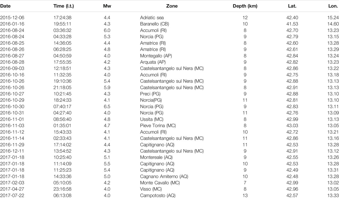
TABLE 1. List of the 29 earthquakes localized within a distance of 150 km from Chieti with M ≥ 4 shown in Figures 5, 6, 9. Seismic events with 4 ≤ M < 5 are omitted when occurred the same day of a seismic event with M ≥ 5, and only the major with 4 ≤ M < 5 is reported when more than one event occurred the same day. Official data are taken from the INGV website at http://terremoti.ingv.it.

FIGURE 1

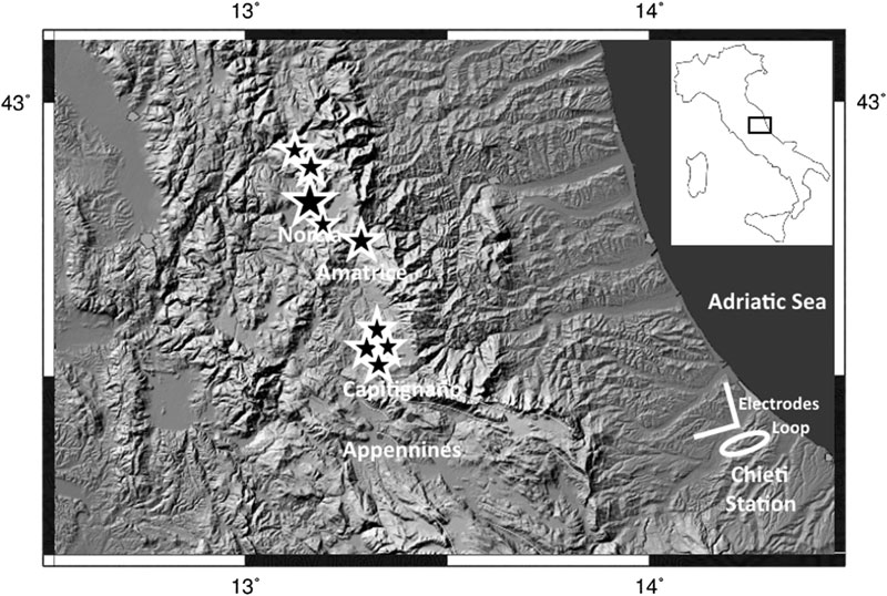
FIGURE 1. The figure shows the azimuth of the magnetic antenna, which was oriented mainly to reduce the 50 Hz noise coming from the local electrical power line as far as possible. Furthermore, the directions of wire electrodes are indicated by white segments. They are located in Chieti, about 70–100 km from the areas of the main shocks (stars).

Electromagnetic Data

Electrical detectors are made up of two principal parts: the outdoor sensor constituted by a pair of orthogonal electrodes with a couple of amplifiers (A1 in Figure 2A) and the indoor real time signal analysis with a recording system realized by a personal computer (IC1 in Figure 2A). The two electrodes oriented along the NNW and WSW directions at Chieti Station are located above the building of the Volcanology Laboratory. The resolution for this electric field detector is calculated to be around 50 μV/m between 10 and 1,000 Hz with a precision of around ±500 μV/m, see Appendix A. The natural electric noise level at Chieti Station in the ELF band varied considerably depending on the meteorological conditions. Spectrum Lab measurements of it ranged from about −90 dB at around 10 Hz to −80 dB at around 100 Hz for fair weather conditions, which corresponds to an electric fields spectral density noise floor of about 10⁻⁴ Vm⁻¹ Hz^−½ (Boldyrev et al., 2016). Spectrum Lab measurements meanwhile around –60 dB with peaks of –40 dB for the whole of the ELF spectrum, corresponding to an electric field spectral density of about 10⁻³ to 10⁻² Vm⁻¹ Hz^−½ (see Appendix A), were made under perturbed meteorological conditions with thunderstorms above or around the station. Typical recordings for fair weather of ELF electric recording at Chieti Station are shown in Figure 3A. The picture displays the dynamic spectra on a color graph which corresponds to both the WSW and NNW direction electrodes, recorded on January 2, 2016 over a 70-min period. Moving along the time direction at constant frequencies which are integer multipliers of 50 Hz, continuous intense phenomena are described by marked horizontal thin lines; they represent the power supply network emission with the first harmonic intensity at about −50 dB. Other less well defined horizontal green/blue lines appear below 50 Hz; these are known as Schumann Resonances (Jackson, 1975) and occur at about 7.6, 14, 19, 24, 31, 37, and 43 Hz. The power intensity increased sporadically by around 10–20 dB, indicated by yellow and red spots above the green band in Figure 3A for frequencies between 50 and 150 Hz. These phenomena were observed during past years by other CIEN stations and the maximum daily intensity of the spots was observed to increase around major earthquake times (Fidani, 2011; Fidani and Martinelli, 2015). The maximum daily intensity of the spots was also observed at Chieti Station and was stored in the IC1 memory. If plotted with respect to the frequency corresponding to the maximum amplitude, the phenomena are circumscribed in a well defined area of the ELF band (see Figure 3B). Green spots with frequencies of around 300, 500 and 900 Hz, which appeared in other positions of Figure 3A, reflected variations in the power absorption of the power network line.

FIGURE 2

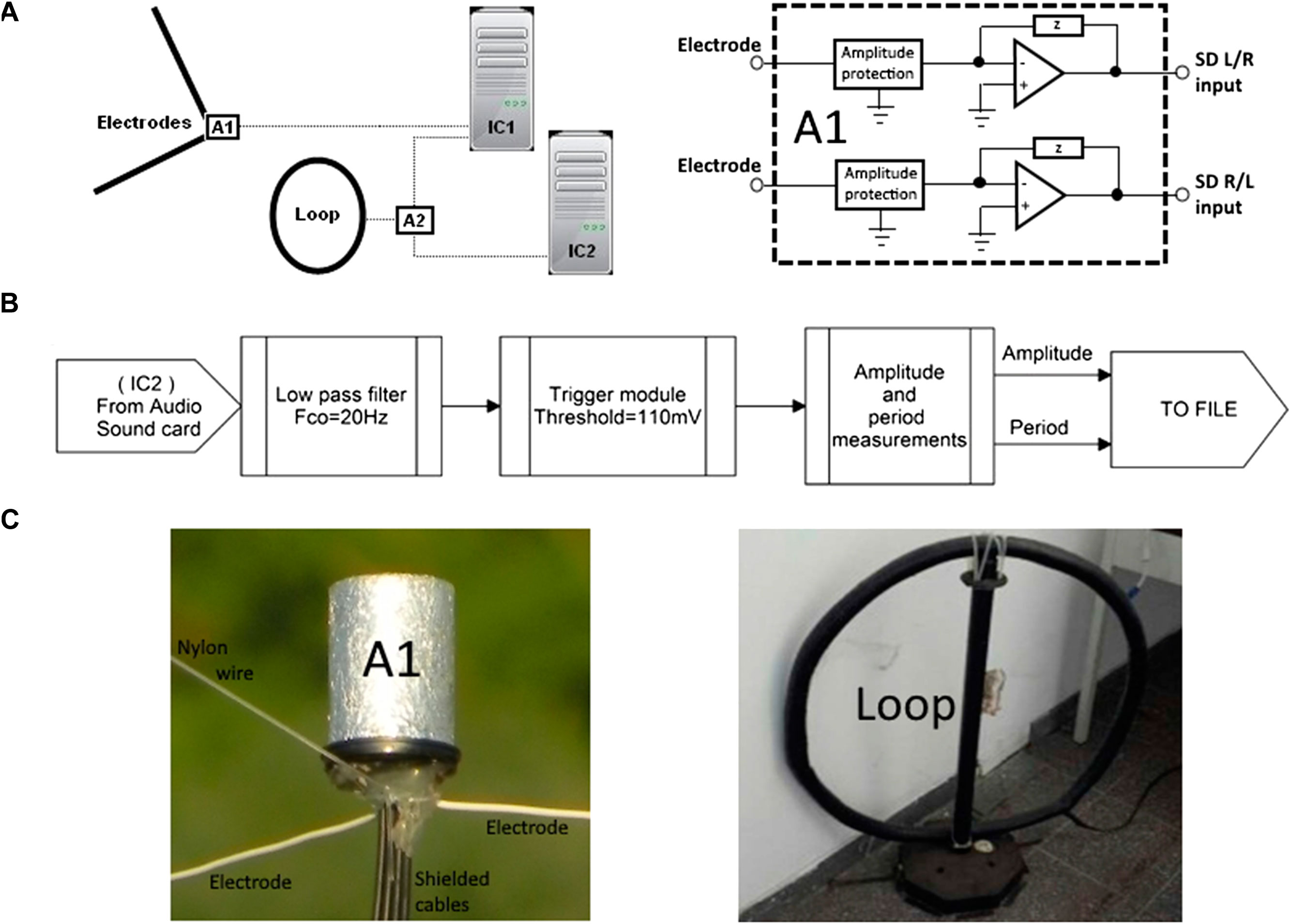
FIGURE 2. A) Configuration of the connections of the electrodes and the loop antenna through the amplifiers A1 and A2 at computers IC1 and IC2, on the left, and the basic scheme of A1 on the right. (B) Simplified block diagram of the laboratory view data acquisition software at IC2 only, consisting of three main blocks starting from the first low-pass filter; the second block is the voltage threshold discriminator, the next block measure the amplitude and the period of the signals. (C) The electric detector made up of electrodes converging in the A1 double amplifier box in the photo on the left, and a particular of the loop in the photo on the right.

FIGURE 3

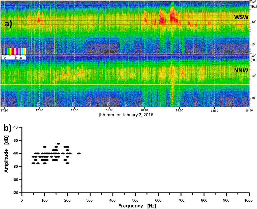
FIGURE 3. A) Dynamic spectra of both WSW and NNW electrodes recorded on January 2, 2016 during the afternoon. Recordings lasted 70 min and show several electric phenomena of natural and anthropological origin. The evident vertical lines covering the entire frequency band and characterized by high intensity are EM waves produced by lightning bolts not too far from the station (Barr et al., 2000). The green band represents the numerous lightning strikes that occurred at distances of thousands of kilometres in the tropics. Red spots are the electrical oscillations. (B) A typical spectrum of maximum daily electric oscillations recorded at IC1 during several months by Spectrum Lab software before the main strike of Norcia. It consists of 81 events of electric oscillations, which are mainly above the noise threshold of –80 dB; all of them fall between 50 and 250 Hz.

The magnetic detector is also made up of two principal parts: the sensor constituted by a loop antenna with an amplifier (A2 in Figure 2A) real-time signal analyser with two recording systems realized by two personal computers (IC1 and IC2 in Figure 2A), both indoors in the building basement. The apparatus receives radio waves in the audio frequency band by magnetic induction at the loop antenna. Then the amplified signal from the output of A2 is divided into two parts, which are connected to two different sound cards of the two different computers: IC1 was used for the comparison with the electrical signals and IC2 was completely dedicated to the magnetic pulse analysis (see Figure 2A). The resolution of this magnetic field detector is around 0.05 nT at 10 Hz with a precision of ±1 nT, see Appendix B. The loop antenna is located in the underground floor of the building. It has been oriented with the axis of symmetry NNW to reduce the 50 Hz noise coming from the local electrical power line in order to turn down the voltage threshold, which is adjustable by software. Electric currents induced in the magnetic loop were amplified and divided into two equal signals to be analyzed by IC1, which was equipped with a supplementary sound card, and by IC2. Dynamic spectra obtained by IC1 analysis revealed a very stable and regular behavior with a uniform noise level that reached −70 dB between 12 and 30 Hz, −80 dB above 30 Hz and −90 dB below 12 Hz. The uniform noise was interrupted almost exclusively by magnetic pulses which were rarely observed during either weak or strong meteorological phenomena and lightning bolt strikes which occurred near Chieti Station. Magnetic pulses appeared like vertical lines in the dynamic spectra, as expected. Power spectra of pulses covered nearly all the frequencies up to several hundreds of hertz, with a 5–10 dB power level greater than the noise level (see Figure 4). The Labview data acquisition software at IC2 allowed to test different settings of the threshold, as well as different filter configurations to evaluate the number of daily triggers. A search of the filter cut-off frequency was implemented, being so the 50 Hz influence coming from the electrical power line was almost completely excluded from data. The acquisition at IC2 had constant parameters between September 2, 2016 and June 28, 2017, when the voltage threshold defined by the Labview data acquisition software was set to 110 mV; corresponding to about 2.5 nT at 10 Hz (see Appendix B), while the filter cut-off frequency was set to 20 Hz, and the data acquisition ran for 24 h per day. Computers IC1 and IC2 for the electrical and magnetic recordings and analysis are located in the underground floor of the building.

FIGURE 4

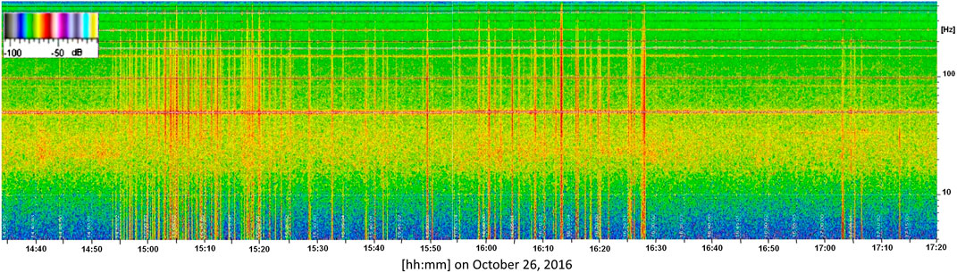
FIGURE 4. Dynamic spectra recorded on 26 October in the afternoon. Recordings lasted 175 min and show a train of magnetic pulses that started at 14:55 LT, indicated by vertical lines; horizontal lines are the traces of 50-Hz power supply harmonics.

Chieti Station was also equipped with a subterranean electrodes system which was installed in September 2010. Electrodes were made up of three square boreholes, 2 m depth, and 1 m width each, aligned to the magnetic field in the NW-SE direction; the center of each borehole is distant 3 m from the other two. Because of the 20° dip in the field surface, the borehole tops are shifted by 1.20 m from the NE borehole to the SW borehole. In the center of each borehole were placed four electrodes, constituted of Fe plates 50 × 50 × 0.5 cm, for a total of 12 electrodes. The first four are on the bottoms of the holes, the others separated by 50 cm of soil levels from each other and from the surface. The acquisition hardware was certified USB DAQ module E14–140 M by L-Card LLC (Bobrovsky et al., 2017). Analysis of the Chieti Station subterranean electrodes database showed impulse-like signals of ground electromagnetic field values measured up to 14 days before the strongest quakes in Central Italy. Furthermore, to compare micro-seismicity with electromagnetic acquisitions, an SR04 EDUGEO three-axis seismograph was recently installed at the same position.

Data Analysis

Spectrograms related to the electric fields were analyzed for a year and half from the beginning of January 2016 up to the end of June 2017. This period was characterized by a lot of gaps in the data, which were caused by power supply interruptions during several time intervals in 2016 and 2017. Gaps in the data occurred in intervals of one or more days, and they exactly corresponds to gaps in spectrograms being the sample frequency of kHz. The ELF bands of electric fields were collected in a time series of the maximum daily intensity of oscillations in both the NNW and the WSW direction. These series of data showed intensity variations with some correspondence with the recorded seismic activity from October 2016 to the beginning of January 2017, as shown below. In fact, electric ELF oscillations at Chieti Station increased in intensity from 10 to 20 dB above the noise level along WSW direction, when strong seismic activity occurred near the station, namely at the time of the Castelsantangelo sul Nera-Norcia (on October 26, 19:10 Mw = 5.4 and 21:18 Mw = 5.9, and on October 30, 07:40 Mw = 6.5, UTC) earthquakes in 2016. The same type of increase in ELF oscillations was detected at the time of the Emilia (Mw = 6.0, Mw = 5.8) earthquakes in 2012 (Fidani and Martinelli, 2015) and at the time of the L’Aquila (Mw = 6.3) earthquake in 2009 (Fidani, 2011). At the same times, behaviors differed between the NNW and WSW components. Namely, a near constant behavior characterized the maximum intensity of ELF oscillations recorded by the NNW electrode. Detected ELF oscillations are indicated by vertical bars in Figures 5A,B. Recordings by the WSW electrode between January 2016 and June 2017 (see Figure 5B) shown a maximum intensity increased since mid-October 2016 and reached a peak a few days after the main shock in Norcia. The daily frequency of oscillations in both the NNW and the WSW direction increased to cover near all days from October to December 2016. Chieti Station data before and after the Amatrice earthquake that occurred on August 24, 2016 (Mw = 6.0), were partially lost because of the power supply shutdown at Chieti University during the vacation period. The Chieti Station has always recorded low ELF activity since 2011, even if less than1 every 3 days and with an average amplitude of around −65 dB for both the NNW and the WSW direction. Amplitudes of ELF oscillations reached about −50 dB around the maximum values; they correspond to induced electric potentials of 360 μV Hz^−½, see Appendix A. Rainy days with elevated electrical activity are also shown in Figure 5C by vertical bars proportional to the daily amount of rain, whereas seismic events are indicated by black circles. No clear correspondence between rain and electric potential measurements is apparent at Chieti Station.

FIGURE 5

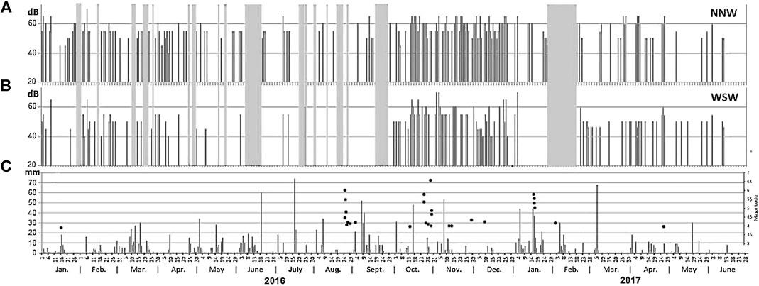
FIGURE 5. The distribution of WSW electric oscillations (A) and the distribution of NNW electric oscillations (B) are indicated by black vertical lines. Rain is indicated by vertical lines in (C), together with strong seismic events, indicated by black circles. Periods of lost data are indicated by gray shadows for both (A,B).

Starting from September 2, 2016, the Labview software saved data for 24 h. On October 25 the daily count below 8 Hz increased significantly above the total average of 29 pulses; then it returned to the typical daily rate on November 24 (Figure 6), which was characterized by an average of six pulses of at least 2.5 nT. A significant decrease in the daily count reached the average value of two when the frequency was below 8 Hz: this occurred between December 18, 2016, and January 10, 2017, when a very high rate of pulses above the threshold of 2.5 nT at 10 Hz (see Appendix B) appeared eight days before the Capitignano earthquakes (Mw = 5.5) on January 18, 2017. From 24 October, several pulses with amplitudes much greater than 2.5 nT were recorded in the frequency band lower than 10 Hz, as shown by the daily spectrum in Figure 7. The same effect was recorded in terms of the daily trigger number, which first increased in the band below 10 Hz, where the detector is less sensitive, and then decreased progressively until it almost disappeared on the day of the mainshock in Norcia (October 30, 2016). It is important to point out that the detector even recorded some pulses with amplitudes greater than 10 nT below 10 Hz, where the typical voltage gain of the amplifier decreases for those frequencies. In fact, a first signal with the amplitude of 53 nT at 6.8 Hz was recorded on October 25, along with a few other pulses recorded at lower frequencies reaching amplitudes beyond 60 nT. Several other pulses with amplitudes greater than 60 nT under 4 Hz, were recorded on the 27, 28 and October 29, 2016, near 80 nT on 29. The number of pulses with amplitudes greater than 2.5 nT increased significantly on 10 and January 12, 2017, when the number of these signals was 3.4 and 2.1 times greater than usual, respectively. Around the average numbers of pulses were also detected on January 11, 13 and 15. During the days preceding the Capitignano earthquake on January 18, 2017, several signals greater than 2.5 nT appeared, mainly between 4 and 10 Hz, as shown in Figure 8. In the same figure, it is possible to see that sometimes several pulses were recorded even below 7 Hz and all were above the voltage threshold. In fact, the day preceding the quake, the antenna received a pulse with a frequency of 4.4 Hz with an amplitude of 45 nT, while at a greater frequency of 16.8 Hz had an amplitude of 10 nT. The day after the mainshock, the detector recorded two big pulses, the first with a frequency of 9.5 Hz and an amplitude of 20 nT, and the second with a frequency of 14 Hz and an amplitude of 31 nT.

FIGURE 6

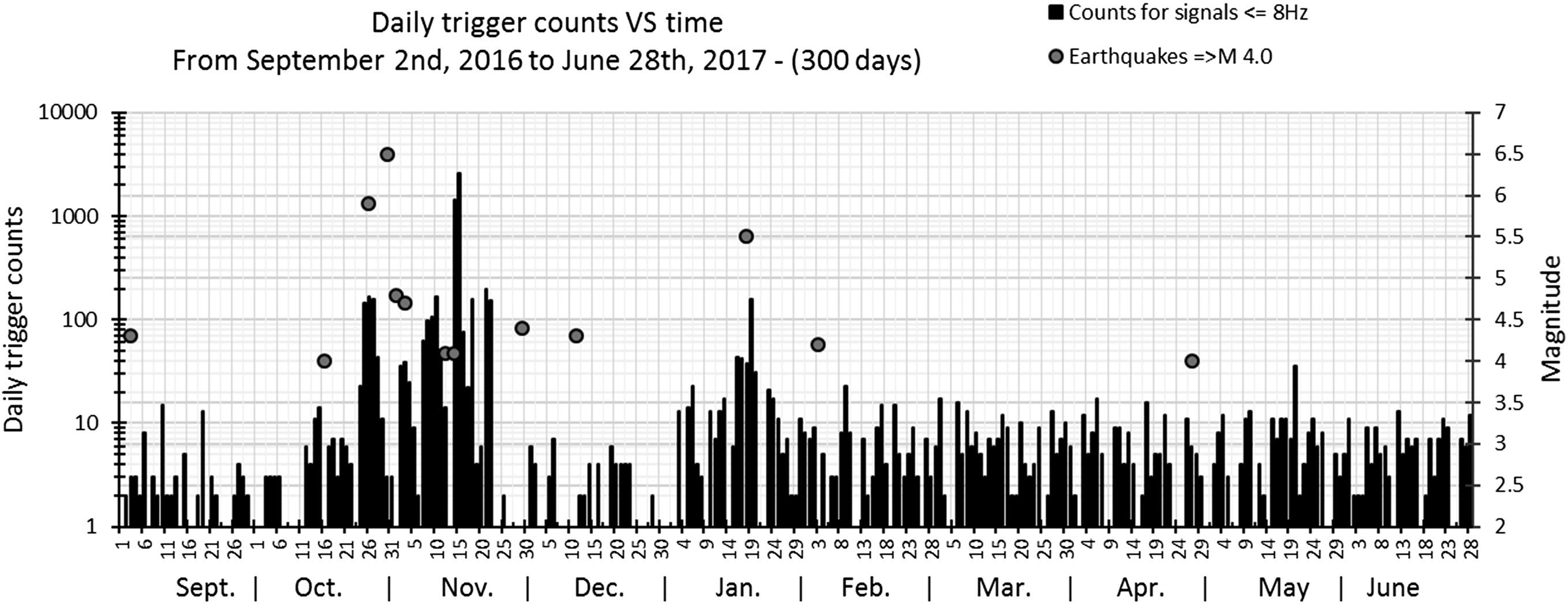
FIGURE 6. Two significant increases of the daily counting rate below 8 Hz were recorded, the first from 25 October to 23 November and then another that appeared from 16 to 20 January. Notice that the plot reports only the biggest daily earthquakes listed in Table 1. The plot reports only the daily biggest earthquakes listed in Table 1 by gray circles.

FIGURE 7

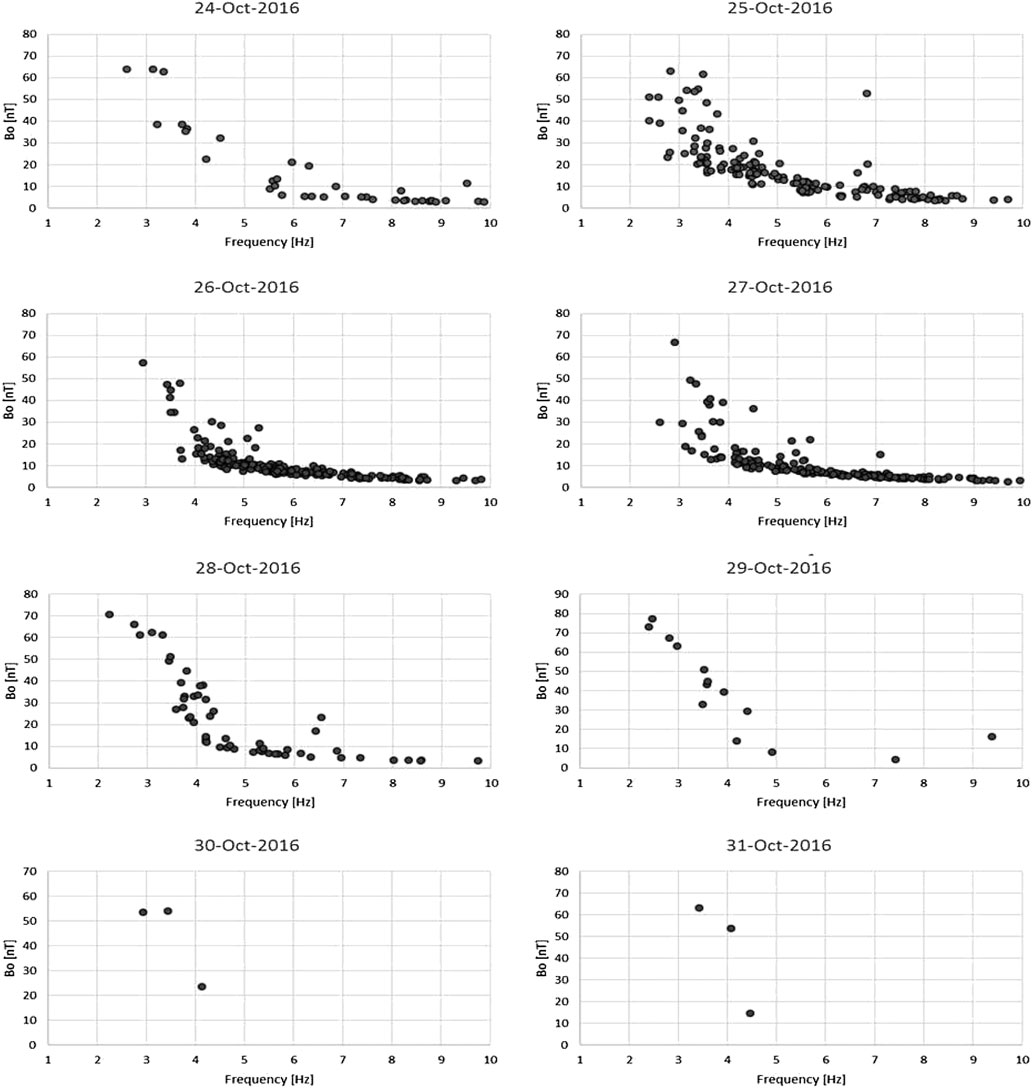
FIGURE 7. The daily spectrum from 24 to October 31, 2016. From 24 October, the detector recorded an increase in the number of pulses below 10 Hz. The detector recorded some pulses with amplitudes near 80 nT between 2 and 3 Hz even though the gain of the preamplifier was lower at those frequencies. It is evident from the above graphs that the magnetic induction threshold is frequency dependent after that the limit of 110 mV was fixed.

FIGURE 8

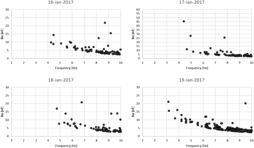
FIGURE 8. The daily spectra from 16 to January 19, 2017. A day before the main shock in Capitignano (January 18, Mw = 5.5), three pulses with amplitudes greater than 20 nT appeared in the band between 4 and 8 Hz and even during the day of the main shock in Capitignano a pulse and the day after two pulses between 3 and 10 Hz.

Spectrograms of the magnetic loop signals obtained by IC1 were saved with frequencies between 4 and 450 Hz in a logarithmic scale, starting from July 21, 2015, to October 31, 2017. Spectrograms of magnetic components evidenced a regular pattern that was interrupted a few times every day by vertical lines; such lines represented the graphic markers of pulses. Magnetic pulses were selected with a 5-dB threshold above the noise level in this representation. The average number of pulses was around eight pulses for day. Daily pulse numbers typically did not increase during strong meteorological perturbations and thunderstorms. There was no evidence of increases in the daily pulse number around the Amatrice main event on August 24, 2016, when the detector was on. It increased slightly on 25 October and increased strongly on 26 October, reaching 45 pulses when two moderate earthquakes of Mw = 5.4 and Mw = 5.9 struck Central Italy about 100 km from the Chieti Station (see Figure 9A). Pulse rates increased about 4 h before the Castelsantangelo sul Nera quakes occurred (on October 26, 19:10 Mw = 5.4 and 21:18 Mw = 5.9, UTC), as shown in Figure 5. The pulse rate increased to 88 on 27 October, decreased to 30 on 28 October, and increased again to 60 on October 29, 2016, the day before the main shock in Norcia (see Figure 9A). After this day, the pulse rate returned to the average value of eight pulses for day in the next days until November 3, 2016, when a new maximum of 92 was reached (see Figure 9A). For the next three weeks, pulse rate maxima appeared at intervals of exactly one week. Therefore, the entire process of weekly increases in pulse rate covered a four-week interval with a total of five maxima. The same pattern appears in Figure 6 as was obtained by IC2 analysis. A new strong pulse rate was measured by IC1 on January 16, 2017, 2 days before the strong seismic swarm of Montereale, L’Aquila, about 70 km from Chieti Station, when 96 daily magnetic pulses were recorded by IC1. A similar peak was observed by IC2 analysis as well. The methodologies performed by IC1 and IC2 were essentially different, as the first was based on FFT with a threshold chosen from the signal power, whereas the other was based on a threshold chosen from the signal amplitude after filtering in signal periods. However, they produced identical results of significant variations in pulse rates. IC2 analysis revealed that the characteristic pulse frequencies reached the upper border of ULF band, where natural phenomena such as geomagnetic activity are able to generate disturbances. The majority of the ULF radiation have magnetospheric origin, thus, the geomagnetic activity of the same period was reported by means of the Ap (downloaded from ftp://ftp.ngdc.noaa.gov/STP/GEOMAGNETICDATA/APSTAR/apindex) and Dst (downloaded from http://wdc.kugi.kyoto-u.ac.jp/dst_final/index.html) indexes (see Figures 9B,C for comparisons with the magnetic pulse number). The Ap index is a measure of the general level of geomagnetic activity over the globe that is related to solar activity such as solar storms and the eleven-year cycle, which produces strong magnetospheric influences (Vassiliadis, 2008). Dst was also considered to take into account sub-storm activity, when geomagnetic perturbations can be of considerable intensity even if concentrated in the ULF band (Echer et al., 2004; Kozyreva et al., 2007). In particular, the sudden negative variations in Dst could be misinterpreted as magnetic pulses when intensity variations exceeded 100 nT. Figures 9A,B show that magnetic pulse maxima do not in general coincide with peaks of the Ap index or with stronger quakes. Even Dst variations are not related to the pulse number according to Figures 9A,C. Finally, statistical correlations were calculated between the magnetic pulses and the Ap index time series (see Supplementary Material), and between the magnetic pulses and the Dst index time series (see the Supplementary Materials). They are reported in Figure 10 left, which show no significant statistical correlations.

FIGURE 9

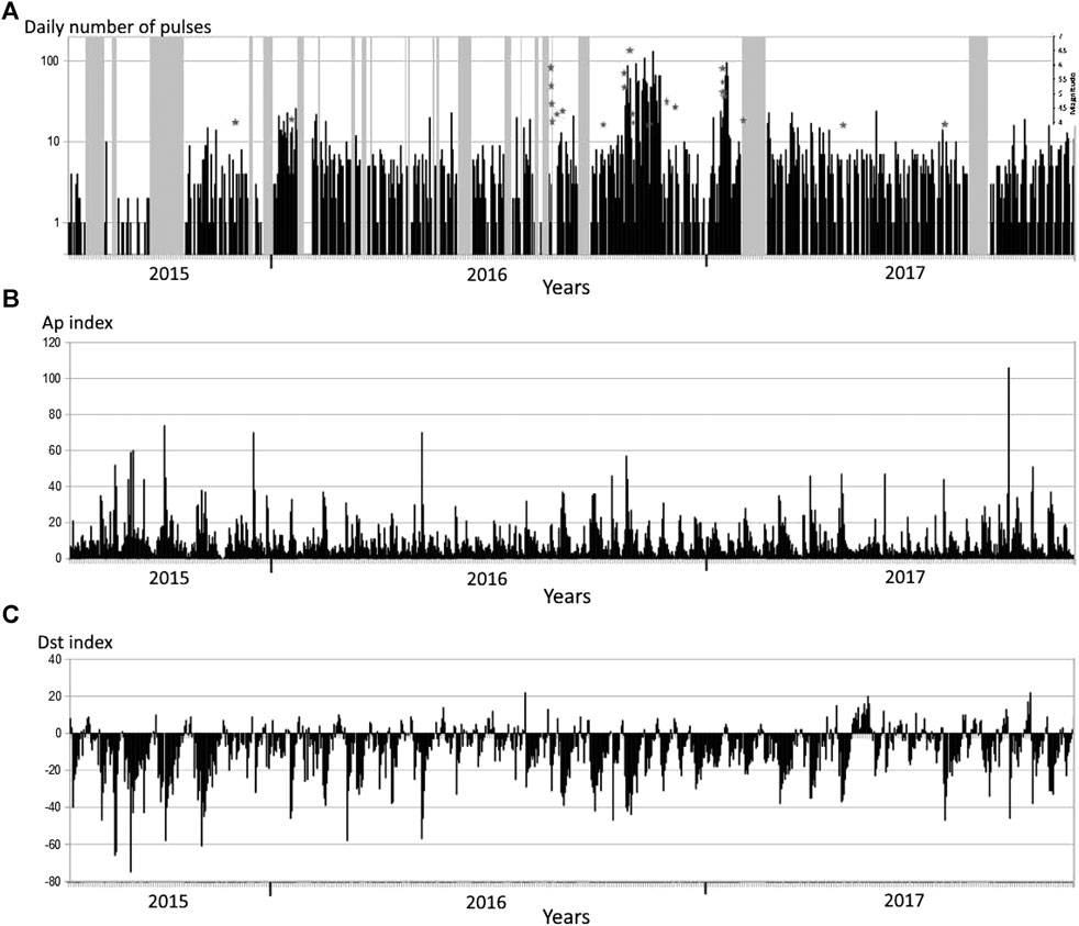
FIGURE 9. The daily number of magnetic pulses recorded by IC1 for the time interval from the end of July 2015 to October 2017 is indicated by vertical lines in (A). Vertical lines in (B,C) describe geomagnetic activity by means of Ap and Dst indexes, respectively. The occurrence of strong seismic events (M ≥ 4) is indicated by grey stars. Periods of lost data are indicated by gray shadows.

FIGURE 10

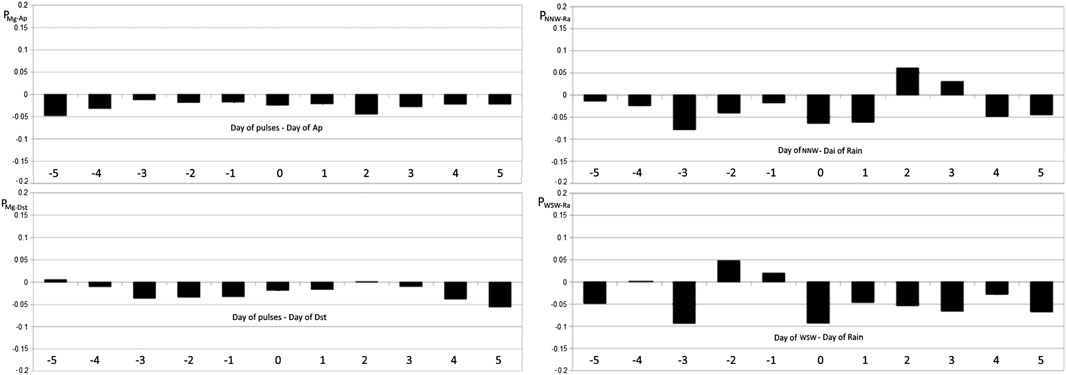
FIGURE 10. Statistical correlations of ±5 days in time differences between magnetic pulses and Ap index time series, and between magnetic pulses and Dst index time series on the left, degree of freedom were 835; between NNW electrical oscillations and rain at Chieti Scalo time series, and between WSW electrical oscillations and rain at Chieti Scalo time series on the right, degree of freedom were 467.

Discussion of Physical Models

Electric and magnetic fields recorded by Chieti Station in 2016 and 2017 evidenced several excesses with respect to the average recordings which occurred around the major seismic events. Indeed, no excesses were recorded around the Amatrice earthquake of Mw = 6.0 on August 24, 2016 for electric or magnetic fields. Even though a significant loss of data occurred days and weeks before this event, first from 5 to 7 August and then from 13 to 21 August, during the 3 days preceding the “main shock” and even during the 6 days afterward, the data acquisition did not record any significant variations of electric or magnetic signals. Moreover, electric and magnetic excesses were recorded around the Castelsantangelo sul Nera earthquake on 26 October (Mw = 5.9), the Norcia earthquake on 30 October (Mw = 6.5), and the Montereale earthquake on 18 January (Mw = 5.5). However, such excesses were detected not exactly on the occurrence of these events but hours and days before and after the quake times. Thus, electromagnetic propagation is not able to justify such time differences, nor did the electric and magnetic recording times coincide with the passage of seismic waves (Yamazaki, 2012) at the position of Chieti Station. Therefore, it seems that any possible physical model connected with charge separation which occurs during rock fractures or seismo-electromagnetic generation must be discarded in this discussion.

Specifically, electric field excesses measured on the occasions of the L'Aquila and Modena earthquakes which occurred in 2009 and 2012, respectively, consisted in ELF oscillations whose intensities reached a maximum during the days around the main shocks (Fidani, 2011; Fidani and Martinelli, 2015). Electric field oscillations in the ELF band with the same spectral pattern as the cited cases were also recorded around Norcia and Capitignano earthquakes, as shown above. In all of the described cases, the intensity excesses of electric oscillations lasted weeks before and after the respective main shocks, with intensity distributions centered around the earthquake times. Therefore, even if some excesses in electric oscillations cannot be excluded around the Amatrice earthquake when loss of data occurred, the recordings show that a distribution centered around the Amatrice earthquake time did not appear. Moreover, the increased density in daily detection of electric oscillations which was observed weeks before and after the L’Aquila 2009, Modena 2012, and Norcia 2016 earthquakes was also observed by the Chieti electric detector around the time of the Amatrice earthquake. Further properties are evidenced in this study concerning electric oscillations with respect to those observed for the L’Aquila and Modena earthquakes, as the intensity of electric oscillations was discriminated between the NNW and WSW directions in this work. Recordings evidenced that intensity variations increased significantly only in the WSW direction, while the density in daily detection increased for both the NNW and the WSW direction.

Regarding the magnetic field, excesses occurred in the number and intensities of magnetic pulses, which exceeded some thresholds. Such excesses were also observed for the L'Aquila earthquake in 2009, by means of a loop located near L'Aquila city (Orsini, 2011), and for the Modena earthquake in 2012 by means of an integrated semiconductor device near Modena [Curcio, 2012 (personal communication)]. Pulses were not observed for the Modena earthquake in 2012, probably because no loops were working at less than 300 km from the epicentre. Excesses in the number of magnetic field pulses were also recorded around Norcia and Capitignano earthquakes (see Figures 6, 9A), while they were not recorded around the Amatrice earthquake (see Figure 9A). Magnetic pulses were recorded with the same data gaps as the electric recordings. As for the electric signals, excesses in the number of magnetic pulse also showed a persistence of several days before and after the L'Aquila, Norcia, and Capitignano earthquakes. Such persistence was not observed around the Amatrice earthquake. Moreover, unlike past works, where magnetic pulses were recorded in the ULF band below 1 Hz (Johnston, 1997), here the harmonic content of pulses was concentrated in the ELF band, around 5 Hz. Finally, magnetic pulses in the ELF band were recently detected for moderate earthquakes reaching intensities of tens of nT, and in some cases beyond 100 nT (Scoville et al., 2015; Kappler et al., 2019).

The intensity and distribution of electric oscillations increased during the same weeks when the number of magnetic pulses increased around the Norcia earthquake, even though there were some differences. WSW electric oscillations increased around October 15, 2016, 11 days before the Castelsantangelo sul Nera events and 15 days before the Norcia event, reached a maximum intensity on 3 November, decreased in the next weeks, and then reached a new maximum on January 10, 2017. The number of magnetic pulses increased on October 25, 2016, reaching a maximum on 28 October and a minimum on November 2, 2016. The number of pulses continued to oscillate with a weekly period at least three more times, reaching an absolute maximum on November 16, 2016, then decreased, and then increased again on 17 January to reach a new maximum on January 19, 2017. Therefore, the ELF band electric activity started to increase about 10 days before the strong events of Castelsantangelo sul Nera and Capitignano, whereas the magnetic pulse activity started to increase about 1 day before strong shocks. A further comparison between electric and magnetic activity using IC1 evidenced the absence of magnetic pulses or oscillations corresponding to the electric oscillations, and the absence of electric oscillations and electric pulses also shifted in time corresponding to magnetic pulses, see Varotsos et al. (2003). More specifically, electric phenomena recorded around the earthquake time represent oscillations lasting from few minutes to tens of minutes with a frequency dispersion of several tens of hertz. Magnetic phenomena recorded around the earthquake time instead represent pulses lasting several tens of milliseconds with a frequency dispersion that is very large. Moreover, although they were both recorded in the ELF band, electric phenomena have a maximum power spectrum around 100 Hz while magnetic phenomena have a maximum power spectrum around and less than 10 Hz. Therefore, the two phenomena observed for the strong earthquakes of both October 2016 and January 2017 did not seem to be directly related to one another. Consequently, the Maxwell equations can be used to verify failure of electric and magnetic recordings at Chieti Station together. They can be used to start with two different electrodynamics models describing observations, and then an attempt will be made to verify if a common cause can be found.

Starting with electric field measurements, the frequencies of electric field oscillations were very well defined in repeated electrical recordings with a persistent behavior of up to tens of minutes, which suggested some relatively stable source. Electric field oscillations were recorded only by one electrode at a time and one station at a time. Measurements suggested localized floating sources in the atmosphere of limited dimensions able to create a local electric field. For these reasons, the source of electric oscillations measured above the ground was thought to have been produced by charged clouds floating in the atmosphere. To evaluate the electric induction on the electrodes due to charged clouds, a comparison with the magnitude of Schumann Resonances phenomena was carried out. Intensities of Schumann Resonances are well defined, for the first at f = 7.4 Hz their induced potential can be estimated to be around 55 μV Hz^−½ (see Appendix A). Potentials induced by charged clouds are evaluated by calculating the average potential along the electrode length as

$V_o=1/L{\displaystyle {\int }_L^{0}V\left(\mathbf{r}\text{,}x\right)dx},(1)$

where the vector r is the distance between the tip of the wire and the center of the cloud. Mathematically, symmetric and dynamically stable charged clouds were proposed (Tennakone, 2011) by balancing electrostatic forces with air pressure, see Figure 11A. This model is attractive because it suggests that with high charge concentrations, corona discharges in the space between the separate charges can render the cloud luminous (Tennakone, 2011). Therefore, it is able to give a response for a class of observations of earthquake lights, ball lightning, which was one of the arguments (Fidani, 2010) that inspired the CIEN for electromagnetic monitoring. Finally, measurements obtained by CIEN allowed the possibility of estimating the electric field E in the atmosphere and its frequency, making it possible to roughly evaluate the dimensions of the charged clouds. Following Appendix A, the cloud separation diameters of opposite charges are evaluated between 108 and 27 cm respectively with the corresponding positive charges ranging between 2.3 × 10⁻⁴ C, in a volume of 6.6 × 10⁵ cm³, and 1.4 × 10⁻⁵ C, in a volume of 7.6 × 10⁴ cm³, respectively. These give average ion concentrations inside the clouds of about 2.2 × 10⁹ and 1.2 × 10⁹ ions/cm³, respectively. They are able to induce an emf along the electrodes which is calculated in Appendix A, it resulted between 2.8 × 10⁻⁵ to 2.8 × 10⁻⁴ V Hz^−½, see Figure 11B. Based on this model and the ratio between induced potentials, it is demonstrated in Appendix A that the electrodes are completely surrounded by negative charge density.

FIGURE 11

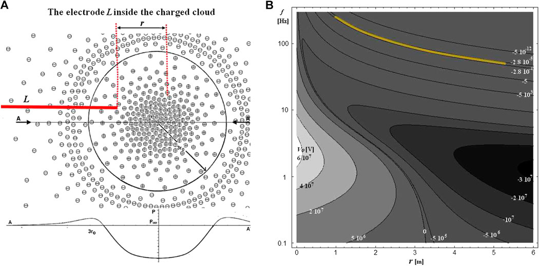
FIGURE 11. The model of spherical charged clouds surrounding an electrode in (A); the cloud radius separating opposite charges is 3r_o, and the pressure P inside the section A-A of the cloud is depicted under it, where P_∞ is the pressure of 1 atmosphere. The retrieved induced potential V_o in the electrode L is shown with respect to the distance r and the oscillation frequencies f retrieved by A6 and A8; the set of possible solutions for cloud distances and frequencies is evidenced on the contour plot of potentials (B).

Electric activity observed during the L'Aquila seismic swarm in 2009 (Fidani, 2011) and during the Modena seismic swarm in 2012 (Fidani and Martinelli, 2015) evidenced that increases in electrical activity occurred in the spring and summer seasons. Meteorological activity also manifested itself more frequently with thunderstorms in spring and summer (Camuffo et al., 2000; Poelman et al., 2014), so past works took into account the possibility that intensity excesses of electric oscillations could be produced by meteorological activity. However, this should be not the case for the 2016 and 2017 Central Italy earthquakes, when electric oscillation excesses appeared between October 2016 and January 2017 (see Figure 6). More specifically, electric oscillations recorded at less than 1 h from rainfall were excluded and a statistical correlation, between the remaining electric oscillations and rainfall at Chieti Station was studied by means of the Pearson product-moment correlation coefficient. The considered period of one and a half years, with 467 effectively recorded days, included 213 days of electric oscillations and 131 rainfall days. The result of the correlation calculation showed that a correlation between the electric oscillations and rainfall is not significantly different from zero (see Figure 10 right). Furthermore, Figures 5A,B show equal density of daily electrical oscillations in the NNW and WSW directions between June 2016 and January 2017, but intensities sound different, with only intensities in the WSW direction having maxima around the Norcia and the Capitignano earthquakes. The difference, which was not evidenced for the L’Aquila and Modena earthquakes, could be linked to wind direction as wind is able to transport clouds of ions. In these pictures, WSW is the direction perpendicular to the Apennine chain.

The model can now be tested to explain magnetic measurements corresponding in time to electric field oscillations, which report no apparent signals emerging from the noise. To this end, it can be considered that in a perfectly spherical symmetric charge distribution, the only direction in which the electric, magnetic, and radiation fields can point is radially outward from the center of the sphere. Moreover, in a radiation field, the electric and magnetic fields must be transverse to the direction of motion, so even if this system is pulsating, it does not produce any radiation. In general, symmetric structures which oscillate radially do not radiate electromagnetic fields due to the symmetry (Heller et al., 2004). However, if a magnetic field detector is in the atmosphere and the charged cloud goes around it, surrounding and encasing it, then the instrument is able to see asymmetric charge movements and to measure variations in the electric and magnetic fields. In the case of Chieti Station, the electric detector can be reached by charged clouds while the magnetic one cannot because it is located underground, at about 20 m from the position of the electric detector. Therefore, it is clear that the Chieti magnetic detector is not able to measure the magnetic component of electric oscillations of charged clouds.

With regard to electric signatures of magnetic pulse recordings, pulses were characterized by a threshold fixed at the Chieti magnetic detector which corresponds to pulse amplitudes exceeding 2.5 nT at 10 Hz, with many recorded pulse amplitudes that reached several tens of nT. To have an initial estimate of the minimal electrical current flowing in the Earth’s crust, a simple model using the Biot-Savart law which considers an infinitely long line conductor that is at some depth in the Earth’s crust was used.

$B_o={\mu }_o{I}_o/\left(2\pi r\right).(2)$

Given that the loop has an axis oriented approximately NNW–SSE, the idealized current flowing parallel to the ground plane that can be induced in the loop will have an approximately WSW-ENE direction, which is perpendicular to the fault strike of Central Italy. This configuration required current variations from at least 1 kA for 2.5 nT to 30 kA for the 80 nT pulses measured before the Norcia earthquake, where the WSW-ENE line is about 75 km from Chieti, and 0.5–10 kA for the Capitignano earthquakes, where the WSW-ENE line is about 40 km from Chieti, in order to produce magnetic induction intensities of up to 50 nT. However, a localized infinitely long line conductor seems a very particular and unlikely condition to be verified in the Earth’s crust to describe magnetic recordings at the Chieti station, as it is not possible to demonstrate that such long line conductors exist underground and currents are not dispersed much earlier. Then, a second model of a finite short horizontal dipole located at the hypo-centre was considered to model magnetic pulses measured at ground (Bortnik et al., 2010). The theoretical approach was developed for an antenna lying near a planar interface (King et al., 1981), which was placed underground in a simple homogeneous medium characterized by its magnetic permeability μ, electric permittivity ε, and electric conductivity σ. The generation of underground electrical currents that may account for the reported observations at large distances of many tens of km can thus be estimated for concentrated sources. The second Maxwell equation system which makes it possible to estimate the magnetic induction generated in a complex permittivity medium Є = ε + i σ/ω can be written as

$\nabla \times \mathbf{E}=i\cdot \omega \cdot \mathbf{B}\text{,}(3)$

$\nabla \times \mathbf{B}=\mu \left(\mathbf{J}-i\cdot \omega \cdot \epsilon \cdot \mathbf{E}\right),$

where the dipole current J_y= δ(x) δ(y) δ(z – d) is located at a depth d in the half-space z > 0, oriented along the x-axis in the WSW-ENE direction at the position x = 0 and y = 0. Thus, the intensity of the radiating element IΔl is a seismo-telluric current which can be constrained by Eq. 3. The system 3 can be solved by a two-dimensional spatial Fourier transform of the fields and imposition of the boundary conditions at the ground, between the atmosphere and soil. The results can be scaled as ∼e^−z/δ (Bortinik et al., 2010), where the skin depth is defined by

$\delta ={\left(\pi f{\mu }_{\text{o}}\sigma \right)}^{-1/2}\text{,}(4)$

while the magnetic field intensity coupled with the loop B_y scales linearly with IΔl. Based on the reported typical pulse lengths, a frequency of f = 2–10 Hz was considered in the following. With regard to the conductivity of the Earth’s crust in Central Italy, the Apennine chain is characterized by a 4 km thick top layer of quartzite with σ = 5 × 10⁻⁴ Ω⁻¹m⁻¹ and underlying gneiss and granite basement with σ = 2.2 × 10⁻³ Ω⁻¹m⁻¹, where μ is approximately 10 μ_o (Juhlin, 1999). These values were confirmed by magneto-telluric studies which obtained a three-strata model that also included superficial soft terrains not present on the Apennines, characterized by values of 0.2 Ω⁻¹m⁻¹ up to 2 km, 3.33 × 10⁻⁴ Ω⁻¹m⁻¹ for the next 3 km, and 2 × 10⁻³ Ω⁻¹m⁻¹ for the next 5 km, respectively (Di Lorenzo et al., 2011). A conductivity of 2.2 × 10⁻³ Ω⁻¹m⁻¹ is used for the homogeneous model considered here as the basement with resulting skin depths δ = 1–2.2 km, depending on f. The top 4 km quartzite layer is characterized by skin depths δ = 2.2–5 km, depending on f. However, ulterior overlying 6 km soft terrains characterized by conductivity of 0.1 Ω⁻¹m⁻¹ and μ = 6 μ_o (Juhlin, 1999), at places eastwards from Apennines such as Chieti, provide skin depths δ = 0.2–0.4 km, depending on f. Magnetic field intensities collected by means of the Chieti loop were calculated to be between 2.5 and 80 nT for the Castelsantangelo sul Nera and Norcia seismic events and between 2.5 and 50 nT for the Capitignano events. Following Bortnik’s work (2010) which is to be used directly in calculating the minimal current necessary to produce magnetic perturbations, a minimum of B_o= 2.5 nT to be observed at Chieti Station was calculated. Taking into account the further estimated loss due to the 6 km soft terrain, it should have required at least IΔl = 4.8 × 10¹⁸ A·m at a distance of 70 km. That is, a 10-km-long radiating element requires a 4.8 × 10¹⁴ A telluric current at a source hypo-centre such as Capitignano. On the other hand, a minimum of B_o= 2.5 nT to be observed at Chieti Station should require IΔl = 2.1 × 10²⁴ A·m at a distance of 100 km. That is, a 10-km-long radiating element requires a 2.1 × 10²⁰ A telluric current at a source hypo-centre such as Norcia. Both values, being minimal values due to the nodes of magnetic distribution, are so elevated as to be unrealistic too. Even if the variable magnetic fields can enter into the atmosphere above the Apennines with intensity losses of 2.5 × 10⁻³ to 1.8 × 10⁻², depending on f, and considering only the geometric loss into the atmosphere, a minimum of 92 and 190 MA current variations would be required to induce signals above the threshold of the magnetometer at Chieti for Capitignano and Norcia, respectively.

Finally, a more realistic model of a distributed electrical current was considered starting from the geological settings of the eastern region in Central Italy. In fact, the Sibillini Mountains where the intense seismic sequence occurred are about 60 km WSW of the Adriatic Sea, which can behave like a very good electric mass, having σ = 5 Ω⁻¹ m⁻¹, toward which any electric charge excess will converge. The geology of the region between mountains and sea is characterized by several kilometres of Laga’s wet clay, which is a good conductor with a conductivity of 0.05–0.2 Ω⁻¹ m⁻¹. Thus, as Laga is a large area extending parallel to both the Adriatic sea and the Apennines, eventually electrical currents between them will be distributed over large sections of the clay deposits. This means that if a charge excess is generated inside the Apennines it will migrate preferentially eastwards, where the large clay area is parallel to the Adriatic coast, and it is thus able to reach lower latitudes equal to Chieti Station latitude (see Figure 12A). These geological considerations are sufficient to suggest a new physical model of a magnetic field created by electrical current density migrating perpendicular to the Adriatic coast. The calculation described in Appendix C retrieves the magnetic induction B_o concatenated with the coil of the instrument and generated by an electrical current density going through a soil section east of the Apennines (see Figure 12A). A current source I_o is located at the earthquake epicentre (x_N,y_N), where x_N = 0 km and y_N = −65 km, while current lines go toward the Adriatic sea, partially passing below Chieti Station at (x_o,y_o), where x_o = −75 km and y_o = 0. The current density is supposed to extends in a section of 2x_i (h − h_o) and is coupled with the loop depending on distance of the idealized infinite line current, and loop reciprocal orientations (see Appendix C). A contour plot of B_o is shown in Figure 12B with respect to x_i extension, using a total current variation of I_o. Supposing I_o is able to extends under the Chieti Station, therefore x_i = x_o, about 40 kA of distributed current variations are sufficient to create variations of B_o = 80 nT, with h_o = 0.1 km and h = 6 km according to geological results for the conductive layer. About 1.3 kA of distributed current variations are necessary to create variations of B_o = 2.5 nT. The electric current density variations to create B_o = 2.5–80 nT can be calculated to about 1.5–44 μA m⁻² at the position of Chieti and, considering the fault length of 20 km and the layer thickness of 6 km, as variations of about 0.011–0.3 mA m⁻² around the epicentre position. The retrieved magnetic induction B_o was found to be little influenced by either h or h_o. The same calculation can be repeated for the Capitignano earthquakes located at x_C = −35 and y_C = −55 km, where the difference between the Chieti Station coordinate and the WSW-ENE line position of such earthquakes was about x_o − x_C = −40 km. In this case, considering x_oi = x_C, the distributed electric current variations can be calculated to create B_o = 2.5–50 nT as about I_o = 0.7–14 kA with 1.4–28 μA m⁻² of current density variations at the position of Chieti.

FIGURE 12

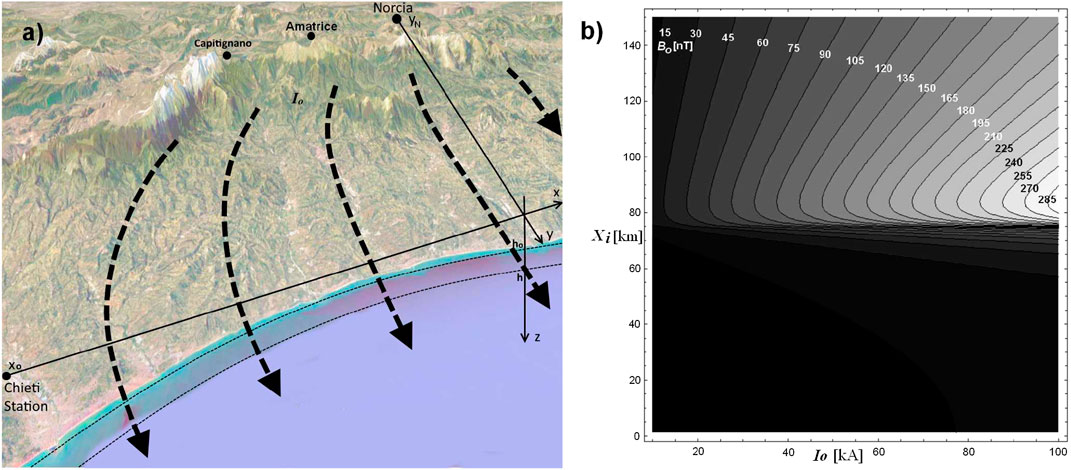
FIGURE 12. The model of electrical currents flowing from the Apennines around the hypo-centre to the Adriatic Sea through the conductive clay layer with the system coordinates in (A); the Chieti Station is at x_o = −75 km while Norcia is at y_N = −65 km. The retrieved magnetic field B_o in the position of Chieti due to the total current I_o, flowing through the conductive layer thickness h–h_o = 5.9 km of width between -x_i and x_i, in a contour plot (B).

Magnetic field pulses are thought of as sudden interruptions of current density in the hypo-centre region to produce current variations and magnetic field variations all around the current density layer. To compare corresponding electric field pulses to magnetic ones, it is necessary to consider that both magnetic and electric detectors are located near the conductor, the conductive layer. In this case, the emitted electromagnetic energy will be principally magnetic with a small electric component, which is due to the conductor’s presence, which reduces the electric field inside it to zero by definition. Indeed, the conductive clay layer is characterized by a finite conductivity (0.1 Ω⁻¹ m⁻¹) and its effect on the electric field can be calculated. Electric fields corresponding to the measured magnetic fields can be written as (Lifstis and Pitaevskij, 1986):

$E_y\approx 2\pi \delta B_x/\left({\mu }_o\lambda \right)\text{,}(5)$

where δ is the skin depth and was evaluated above to be between 0.5 and 1.1 km and λ is the wavelength of the electromagnetic emission that is equal to 30,000 km at 10 Hz and 150,000 km at 2 Hz. Electric field pulse intensities are therefore calculated to be in the range between 2.5 and 4 μV m⁻¹, for greatest pulses of Capitignano and Norcia earthquakes, respectively, around 2–4 Hz. These values are well under the noise level of the electric field and should not be revealed by electric detectors used in this experiment in accordance with the results.

A possible common cause for both observed magnetic and electric measurements with strong earthquakes it is premature at this stage of research. However, some specific model of electrified CO₂ gases passing through the newly created fracture surface of the rock can be considered (Enemoto et al., 2017). Electrified gases are able to produce electric charge excesses in the crust and atmosphere and to generate pressure-impressed current/electric dipoles (Enemoto et al., 2012). Another possible model is the hypotheses of the Lithosphere-Atmosphere-Ionosphere Coupling (Pulinets, 2011; Pulinets and Ouzounov, 2011). It can unite the gaseous emissions before earthquake, charged clouds and thermal anomalies in the common chain, where the key role plays the process of ionization of atmospheric gases (Pulinets et al., 2015). This ionization is provided by α-active radon released over active tectonic faults and tectonic plates borders. Pulses of electrified gases could be responsible for electric charged clouds in the atmosphere and electrical current variations in the crust.

Conclusions

Continuous recordings of non stationary electric fields and magnetic fields with frequencies in the band (3–300 Hz) evidenced specific signals which were exceptional in number and intensity at Chieti Station between 2016 and 2017. Electric anomalies consisting of oscillations of up to a few hundred hertz did not correlate with meteorological lightning and rainfall. Magnetic anomalies consisting of pulses with characteristic frequencies up to 10 Hz did not correlate with Dst and Kp indexes. Nine strong earthquakes distributed in three main periods struck Central Italy in August 2016, October 2016, and January 2017. Events that occurred in October 2016 and January 2017 were preceded by increases in electric oscillations weeks beforehand and were preceded by increases in the number of magnetic pulses 1 day before. It was discussed that the duration of electric oscillations and magnetic pulses lasted for several days and weeks around the earthquake times. Therefore, the Amatrice earthquake in August 2016 seemed to be not accompanied by increased electric magnitude and pulse number even though the data from Chieti Station show gaps during the days around the time of that earthquake.

The electric field components along the WSW and NNW directions showed a gradually increasing number of horizontal electric oscillations. Specifically, the WSW component of the electric field perpendicular to the Apennine chain was characterized by an increase in intensity since mid-October 2016, a maximum in electric intensity occurred on November 2, 2016, and a second maximum of the same intensity on January 6, 2017, about 10 days before the Capitignano shocks. The number of days with electric oscillations also increased during the same period. In contrast, the NNW component of the electric field parallel to the Apennine chain was not characterized by intensity increases but only by the number of days on which electric oscillations increased, from middle of October to the end of December 2016. These results are in agreement with observations made on the occasions of the L'Aquila 2009 (Mw = 6.3) and the Emilia 2012 (Mw = 6.0) earthquakes, when increases of electric oscillations were recorded by Fermo and Zocca stations, respectively.

The magnetic data analysis at Chieti Station, performed through two independent sample systems of the same signal, and two different methods made by Labview and Spectrum Lab programs, shows that 6 days before the earthquake of Norcia and 1 day before the Castelsantangelo sul Nera earthquakes, a large number of pulses were recorded in the ELF band below 10 Hz with amplitudes mostly in the range of 2.5–80 nT, which almost disappeared on the day that the main shock (Mw = 6.5) occurred in Norcia, October 30, 2016. Furthermore, 1 day before the main shock occurred in Capitignano (Mw = 5.5) on January 18, 2017, a larger number of pulses started to be recorded with amplitudes mostly in the range of 2.5–50 nT, and the number then decreased the day after the main shock. These kinds of magnetic signals were already recorded before the L’Aquila (Mw = 6.3) earthquake that occurred on April 6, 2009 (Orsini, 2011), and should be considered to verify their recurrence in sufficiently large number of strong earthquakes.

Physical models were developed to allow for an interpretation of the electric and the magnetic measurements. The model for electric oscillations consisted of charged clouds kept together by atmospheric pressure holes which yielded a stable structure able to oscillate. This model was able to describe the lack of corresponding magnetic components from the loop detector. It was not able to describe differences between WSW measurements and NNW measurements. Data recorded in the other CIEN stations was used up to now exclusively to verify that electric oscillations are not coincident in time and amplitude at different positions, confirming to be local phenomena. The model for magnetic pulses consisted of diffused underground electrical currents between the Apennines and the Adriatic Sea. Furthermore, following this model, the amplitudes and the increased trigger counts recorded before the earthquakes could even be related to the distance from the epicentres to the antenna, which was about 70 km for the Capitignano earthquake epicentre and about 100 km for the Norcia earthquake epicentre. In a model constrained by the geology of the area, a clay conductive layer was able to drive charge excess into the Adriatic Sea, and therein also underneath the Chieti station. The current required to induce detectable pulses is greater than 1 kA, and is greater than 40 kA for strongest pulses, which is of the same order than previous estimated (Bortnik et al., 2010).

The two models, of charged clouds and diffused currents, are self-consistent. Spherically symmetric charged clouds are unable to radiate electromagnetic energy, according with the lack of corresponding magnetic components from the coil magnetometer. Diffused electric currents in the crust are able to describe the lack of corresponding electrical components from the electric field detector as energy was principally concentrated in the magnetic field near the conductive layer. Signal to noise ratio limits of two instruments are consistent with measurements of natural signals such as Schumann Resonances. Common-mode noise generated in the ionosphere/magnetosphere was quantified and considered through geomagnetic indexes. The two different models used for electrical oscillations and magnetic pulses have not yet assigned a common cause, although upwards migrating fluids offer some well-founded answers.

Data Availability Statement

The datasets generated for this study are available on request to the corresponding author.

Author Contributions

CF is the coordinator of the work and he interpreted the data. MO is the acquisition data expert of the work and helped the first author to interpret the data. GI and NV monitored the acquisitions and the laboratory. FS helped the coordination of the work and revised it.

Conflict of Interest

The authors declare that the research was conducted in the absence of any commercial or financial relationships that could be construed as a potential conflict of interest.

Acknowledgments

The authors are grateful to Joerg Renner for his valuable comments.

Supplementary Material

The Supplementary Material for this article can be found online at: https://www.frontiersin.org/articles/10.3389/feart.2020.536332/full#supplementary-material

References

Baratta, M. (1891). “Catalogo dei fenomeni elettrici e magnetici apparsi durante i principali terremoti,”in Rendiconti della Società Italiana di Elettricità pel progresso degli studi e delle applicazioni, Milano, Italy: Tip. Lamperti di G. Rozza, Vol. 1-anno XIII, 15.

Google Scholar

Baratta, M. (1901). I Terremoti di’Italia: saggio di storia, geografia e bibliografia sismica italiana con 136 sismocartogrammi. Editor A. Forni (East Lansing, MI: Michigan State University), 950.

Google Scholar

Barr, R., Jones, D. L., and Rodger, C. J. (2000). ELF and VLF radio waves. J. Atmos. Sol. Terr. Phys. 62 (17), 1689–1718. doi:10.1016/s1364-6826(00)00121-8

CrossRef Full Text | Google Scholar

Biagi, P. F., Castellana, L., Maggipinto, T., Loiacono, D., Schiavulli, L., et al. (2009). A pre seismic radio anomaly revealed in the area where the Abruzzo earthquake (M = 6.3) occurred on 6 April 2009. Nat. Hazards Earth Syst. Sci. 9, 1551–1556. doi:10.5194/nhess-9-1551-2009

CrossRef Full Text | Google Scholar

Biagi, P. F., Ermini, A., and Kingsley, S. P. (2001). Disturbances in LF radio signals and the Umbria-Marche (Italy) seismic sequence in 1997–1998. Phys. Chem. Earth C 26 (10–12), 755–759. doi:10.1016/s1464-1917(01)95021-4

CrossRef Full Text | Google Scholar

Bleier, T., Dunson, C., Maniscalco, M., Bryant, N., Bambery, R., and Freund, F. (2009). Investigation of ULF magnetic pulsations, air conductivity changes and infra red signatures associated with the 30 October Alum Rock M5.4 earthquake. Nat. Hazards Earth Syst. Sci. 9 (2), 585–603. doi:10.5194/nhess-9-585-2009

CrossRef Full Text | Google Scholar

Bobrovskiy, V. S., Stoppa, F., Nicoli, L., and Losyeva, Y. (2017). Nonstationary electrical activity in the tectonosphere-atmosphere interface retrieving by multielectrode sensors: case study of three major earthquakes in Central Italy with M > 6. Earth Sci. India 10, 269–285. doi:10.1007/s12145-017-0296-4.

CrossRef Full Text | Google Scholar

Boldyrev, A. I., Vyazilov, A. E., Ivanov, V. N., Kemaev, R. V., Korovin, V. Y., Melyashinskii, A. V., et al. (2016). Registration of weak ULF/ELF oscillations of the surface electric field strength. Geomagn. Aeron. 56, 503–512. doi:10.1134/s0016793216040034

CrossRef Full Text | Google Scholar

Bortnik, J., Bleier, T. E., Dunson, C., and Freund, F. (2010). Estimating the seismotelluric current required for observable electromagnetic ground signals. Ann. Geophys. 28, 1615–1624. doi:10.5194/angeo-28-1615-2010

CrossRef Full Text | Google Scholar

Brozzetti, F., and Lavecchia, G. (1994). Seismicity and related extensional stress field: The case of the Norcia Seismic Zone (Italy). Annales Tectonicae, 8, 36–57.

Google Scholar

Brozzetti, F., Boncio, P., Cirillo, D., Ferrarini, F., de Nardis, R., Testa, A., et al. (2019). High‐resolution fieldmapping and analysis of the August‐October 2016 coseismic surface faulting (central Italy earthquakes): Slip distri-bution, parameterization, and comparison with global earthquakes. Tectonics 38, 417–439. doi:10.1029/2018TC005305

CrossRef Full Text | Google Scholar

Calderoni, G., Rovelli, A., and Di Giovambattista, R. (2017). Rupture directivity of the strongest 2016–2017 Central Italy earthquakes. J. Geophys. Res. Solid Earth 122, 9118–9131. doi:10.1002/2017JB014118

CrossRef Full Text | Google Scholar

Camuffo, D., Cocheo, C., and Enzi, S. (2000). Seasonality of instability phenomena (hailstorms and thunderstorms) in Padova, northern Italy, from archive and instrumental sources since AD 1300. Holocene 10 (5), 635–642. doi:10.1191/095968300666845195

CrossRef Full Text | Google Scholar

Cinti, F. R., Faenza, L., Marzocchi, W., and Montone, P. (2004). Probability map of the next M ≥ 5.5 earthquakes in Italy. Geochem. Geophys. Geosyst. 5 (11). doi:10.1029/2004gc000724

CrossRef Full Text | Google Scholar

Di Lorenzo, C., Palangio, P., Santarato, G., Meloni, A., Villante, U., and Santarelli, L. (2011). Non-inductive components of electromagnetic signals associated with L’Aquila earthquake sequences estimated by means of inter-station impulse response functions. Nat. Hazards Earth Syst. Sci. 11, 1047–1055. doi:10.5194/nhess-11-1047-2011

CrossRef Full Text | Google Scholar

Echer, E., Alves, M. V., and Gonzalez, W. D. (2004). Geoeffectiveness of interplanetary shocks during solar minimum (1995–1996) and solar maximum (2000). Sol. Phys. 221, 361–380. doi:10.1023/B:SOLA.0000035045.65224.f3

CrossRef Full Text | Google Scholar

Enomoto, Y. (2012). Coupled interaction of earthquake nucleation with deep Earth gases: a possible mechanism for seismo-electromagnetic phenomena. Geophys. J. Int. 191 (3), 1210–1214. doi:10.1111/j.1365-246X.2012.05702.x

CrossRef Full Text | Google Scholar

Enomoto, Y., Tsutsumi, A., Fujinawa, Y., Kasahara, M., and Hashimoto, H. (1991). Candidate precursors: pulse-like geoelectric signals possibly related to recent seismic activity in Japan. Geophys. J. Int. 131, 485–494. doi:10.1111/J.1365-246X.1997.TB06592.X

CrossRef Full Text | Google Scholar

Enomoto, Y., Yamabe, T., and Okumura, N. (2017). Causal mechanisms of seismo-EM phenomena during the 1965–1967 Matsushiro earthquake swarm. Sci. Rep. 7, 44774. doi:10.1038/srep44774

CrossRef Full Text | Google Scholar

Ferrarini, F., Lavecchia, G., de Nardis, R., and Brozzetti, F. (2015). Fault geometry and active stress from earthquakes and field geology data analysis: the Colfiorito 1997 and L’Aquila 2009 cases (Central Italy). Pure Appl. Geophys. 172 (5), 1079–1103. doi:10.1007/s00024-014-0931-7

CrossRef Full Text | Google Scholar

Fidani, C., and Martinelli, G. (2015). A possible explanation for electric perturbations recorded by the Italian CIEN stations before the 2012 Emilia earthquakes. Boll. Geofis. Teor. Appl. 56, 211–226. doi:10.4430/bgta0145

CrossRef Full Text | Google Scholar

Fidani, C. (2010). The earthquake lights (EQL) of the 6 April 2009 Aquila earthquake, in Central Italy. Nat. Hazards Earth Syst. Sci. 10, 967–978. doi:10.5194/nhess-10-967-2010

CrossRef Full Text | Google Scholar

Fidani, C. (2011). The Central Italy electromagnetic network and the 2009 L’Aquila earthquake: observed electric activity. Geosci. J. 1 (1), 3–25. doi:10.3390/geosciences1010003

CrossRef Full Text | Google Scholar

Galli, P., Castenetto, S., and Peronace, E. (2017). The macroseismic intensity distribution of the 30 October 2016 earthquake in Central Italy (M_w 6.6): seismotectonic implications. Tectonics 36, 2179–2191. doi:10.1002/2017TC004583

CrossRef Full Text | Google Scholar

Gradshteyn, I. S., and Ryzhik, I. M. (2007). Table of integrals, series, and products. Editors Jeffrey, A. Jeffrey and D. Zwillinger (Burlington, MA: Academic Press).

Google Scholar

Grosz, A., Paperno, E., Amrusi, S., and Zadov, B. (2011). A three-axial search coil magnetometer optimized for small size, low power, and low frequencies. IEEE Sens. J. 11 (4), 1088–1094. doi:10.1109/jsen.2010.2079929

CrossRef Full Text | Google Scholar

Han, P., Hattori, K., Hirokawa, M., Zhuang, J., Chen, C.-H., Febriani, F., et al. (2014). Statistical analysis of ULF seismomagnetic phenomena at Kakioka, Japan, during 2001–2010. J. Geophys. Res. Space Phys. 119 (6), 4998–5011. doi:10.1002/2014ja019789

CrossRef Full Text | Google Scholar

Hayakawa, M., Kasahara, Y., Nakamura, T., Muto, F., Horie, T., et al. (2010). A statistical study on the correlation between lower ionospheric perturbations as seen by subionospheric VLF/LF propagation and earthquakes. J. Geophys. Res. 115, A09305. doi:10.1029/2009JA015143

CrossRef Full Text | Google Scholar

Heller, L., Ranken, D., Best, E., Ranken, D., and Best, E. (2004). The magnetic field inside special conducting geometries due to internal current. IEEE Trans. Biomed. Eng. 51 (8), 1310–1318. doi:10.1109/tbme.2004.827554

CrossRef Full Text | Google Scholar

Jackson, J. D. (1975). Classical electrodynamics. 1st Edn. Hoboken, NJ: Wiley and Sons Inc., 363.

Google Scholar

Johnston, M. J. S. (1997). Review of electric and magnetic fields accompanying seismic and volcanic activity. Surv. Geophys. 18, 441–476. doi:10.1023/a:1006500408086

CrossRef Full Text | Google Scholar

Juhlin, C. (1999). Geotechnology: Geophysical Methods.

Google Scholar

Kamogawa, M., Liu, J.-Y., Fujiwara, H., Chuo, Y.-J., Tsai, Y.-B., Hattori, K., et al. (2004). Atmospheric field variations before the march 31, 2002 M6.8 earthquake in taiwan. Terr. Atmos. Ocean Sci. 15 (3), 397–412. doi:10.3319/tao.2004.15.3.397(ep)

CrossRef Full Text | Google Scholar

Kappler, K. N., Schneider, D. D., MacLean, L. S., Bleier, T. E., and Lemon, J. J. (2019). An algorithmic framework for investigating the temporal relationship of magnetic field pulses and earthquakes applied to California. Comput. Geosci. 133, 104317. doi:10.1016/j.cageo.2019.104317

CrossRef Full Text | Google Scholar

King, R. W. P., Smith, G. S., Owens, M., and Wu, T. T. (1981). Antennas in Matter: Fundamentals, Theory and Applications. Cambridge, MA: MIT Press.

Google Scholar

Kozyreva, O., Pilipenko, V., Engebretson, M. J., Yumoto, K., Watermann, J., and Romanova, N. (2007). In search of a new ULF wave index: comparison of Pc5 power with dynamics of geostationary relativistic electrons. Planet. Space Sci. 55, 755–769. doi:10.1016/j.pss.2006.03.013

CrossRef Full Text | Google Scholar

Kulak, A., Kubisz, J., Klucjasz, S., Michalec, A., Mlynarczyk, J., Nieckarz, Z., et al. (2014). Extremely low frequency electromagnetic field measurements at the hylaty station and methodology of signal analysis. Radio Sci. 49, 361–370. doi:10.1002/2014rs005400

CrossRef Full Text | Google Scholar

Larkina, V. I., Migulin, V. V., Molchanov, O. A., Kharkov, I. P., Inchin, A. S., and Schvetcova, V. B. (1989). Some statistical results on very low frequency radiowave emissions in the upper ionosphere over earthquake zones. Phys. Earth Planet. In. 57 (1–2), 100–109. doi:10.1016/0031-9201(89)90219-7

CrossRef Full Text | Google Scholar

Lavecchia, G., Adinolfi, G. M., de Nardis, R., Ferrarini, F., Cirillo, D., Brozzetti, F., et al. (2016a). Multidisciplinary inferences on a newly recognized active eastdipping extensional system in Central Italy. Terra. Nova. 29 (1) 77–89. doi:10.1111/ter.12251

CrossRef Full Text | Google Scholar

Lavecchia, G., Castaldo, R., de Nardis, R., De Novellis, V., Ferrarini, F., Pepe, S., et al. (2016b). Ground deformation and source geometry of the 24 August 2016 Amatrice earthquake (Central Italy) investigated through analytical and numerical modeling of DInSAR measurements and structural-geological data. Geophys. Res. Lett. 43, 389. doi:10.1002/2016GL071723

CrossRef Full Text | Google Scholar

Lavecchia, G., Ferrarini, F., Brozzetti, F., deNardis, R., Boncio, P., and Chiaraluce, L. (2012). From surface geology to aftershock analysis: constraints on the geometry of the L’Aquila 2009 seismogenic fault system. Ital. J. Geosci. 131 (3), 330–347. doi:10.3301/IJG.2012.24

CrossRef Full Text | Google Scholar

Lifstis, E. M., and Pitaevskij, L. P. (1986). Elettrodinamica dei Mezzi Continui. Moscow, Russia: Mir, 655.

Google Scholar

Molchanov, O. A., and Hayakawa, M. (1999). Subionospheric VLF signal perturbations possibly related to earthquakes. J. Geophys. Res. 103, 17489–17504. doi:10.1029/98JA00999

CrossRef Full Text | Google Scholar

Němec, F., Santolík, O., and Parrot, M. (2009). Decrease of intensity of ELF/VLF waves observed in the upper ionosphere close to earthquakes: a statistical study. J. Geophys. Res. 114, A04303. doi:10.1029/2008JA013972

CrossRef Full Text | Google Scholar

Orsini, M. (2011). Electromagnetic anomalies recorded before the earthquake of L’Aquila on April 6, 2009. Bollettino di Geofisica Teorica e Applicata 52 (1), 123–130.

Google Scholar

Ouzounov, H., Büttner, R., and Zimanowski, B. (2002). Seismo-electrical effects: experiments and field measurements. Appl. Phys. Lett. 80, 334–336. doi:10.1063/1.1431693

CrossRef Full Text | Google Scholar

Parrot, M. (1994). Statistical study of ELF/VLF emissions recorded by a low-altitude satellite during seismic events. J. Geophys. Res. 99, 23339–23347. doi:10.1029/94ja02072

CrossRef Full Text | Google Scholar

Poelman, D. R., Schulz, W., Diendorfer, G., and Bernardi, M. (2014). “European cloud-to-ground lightning characteristics,” in Proceedings of the International Conference on Lightning Protection (ICLP), Shanghai, China, October 11–18, 2014 (IEEE).

Google Scholar

Pulinets, S. A., Ouzounov, D. P., Karelin, A. V., and Davidenko, D. V. (2015). Physical bases of the generation of short-term earthquake precursors: a complex model of ionization-induced geophysical processes in the lithosphere-atmosphere-ionosphere-magnetosphere system. Geomagn. Aeron. 55 (4), 521–538. doi:10.1134/s0016793215040131

CrossRef Full Text | Google Scholar

Pulinets, S., and Ouzounov, D. (2011). Lithosphere-atmosphere-ionosphere coupling (LAIC) model-an unified concept for earthquake precursors validation. J. Asian Earth Sci. 41 (4–5), 371–382. doi:10.1016/j.jseaes.2010.03.005

CrossRef Full Text | Google Scholar

Pulinets, S. (2011). The synergy of earthquake precursors. Earthq. Sci. 24 (6), 535–548. doi:10.1007/s11589-011-0815-1

CrossRef Full Text | Google Scholar

Schekotov, A., Izutsu, J., and Hayakawa, M. (2015). On precursory ULF/ELF electromagnetic signatures for the Kobe earthquake on April 12, 2013. J. Asian Earth Sci. 114, 305–311. doi:10.1016/j.jseaes.2015.02.019

CrossRef Full Text | Google Scholar

Scoville, J., Heraud, J., and Freund, F. (2015). Pre-earthquake magnetic pulses. Nat. Hazards Earth Syst. Sci. 15, 1873–1880. doi:10.5194/nhess-15-1873-2015

CrossRef Full Text | Google Scholar

Tennakone, K. (2011). Stable spherically symmetric static charge separated configurations in the atmosphere: implications on ball lightning and earthquake lights. J. Electrost. 69, 638–640. doi:10.1016/j.elstat.2011.08.005

CrossRef Full Text | Google Scholar

Uyeda, S., Nagao, T., and Kamogawa, M. (2009). Short-term earthquake prediction: current status of seismo-electromagnetics. Tectonophysics 470, 205–213. doi:10.1016/j.tecto.2008.07.019

CrossRef Full Text | Google Scholar

Varotsos, P., and Alexopoulos, K. (1984a). Physical properties of the variations of the electric field of the earth preceding earthquakes, I. Tectonophysics 110, 73–98. doi:10.1016/0040-1951(84)90059-3

CrossRef Full Text | Google Scholar

Varotsos, P., and Alexopoulos, K. (1984b). Physical properties of the variations of the electric field of the earth preceding earthquakes. II. determination of epicenter and magnitude. Tectonophysics 110, 99–125. doi:10.1016/0040-1951(84)90060-x

CrossRef Full Text | Google Scholar

Varotsos, P., and Alexopoulos, K. (1987). Physical properties of the variations of the electric field of the Earth preceding earthquakes, III. Tectonophysics 188, 321–347. doi:10.1016/0040-1951(84)90060-X

CrossRef Full Text | Google Scholar

Varotsos, P., and Lazaridou, M. (1991). Latest aspects of earthquake prediction in Greece based on seismic electric signals. Tectonophysics 136, 335–339. doi:10.1016/0040-1951(91)90462-2

CrossRef Full Text | Google Scholar

Varotsos, P. A., Sarlis, N. V., and Skordas, E. S. (2003). Electric fields that “arrive” before the time derivative of the magnetic field prior to major earthquakes. Phys. Rev. Lett. 91 (14), 148501. doi:10.1103/physrevlett.91.148501

CrossRef Full Text | Google Scholar

Varotsos, P. A., Sarlis, N. V., Skordas, E. S., and Lazaridou, M. S. (2007). Electric pulses some minutes before earthquake occurrences. Appl. Phys. Lett. 90, 064104. doi:10.1063/1.2450779

CrossRef Full Text | Google Scholar

Vassiliadis, D. (2008). Response of the radiation belt electron flux to the solar wind velocity: parameterization by radial distance and energy. J. Atmos. Sol. Terr. Phys. 70 (14), 1810–1828. doi:10.1016/j.jastp.2008.05.019

CrossRef Full Text | Google Scholar

Yamazaki, K. i. (2012). Estimation of temporal variations in the magnetic field arising from the motional induction that accompanies seismic waves at a large distance from the epicentre. Geophys. J. Int. 190, 1393–1403. doi:10.1111/j.1365-246x.2012.05586.x

CrossRef Full Text | Google Scholar

Zhang, X., Shen, X., Parrot, M., Zeren, Z., Ouyang, X., Liu, J., et al. (2012). Phenomena of electrostatic perturbations before strong earthquakes (2005–2010) observed on DEMETER. Nat. Hazards Earth Syst. Sci. 12, 75–83. doi:10.5194/nhess-12-75-2012

CrossRef Full Text | Google Scholar