Instrument Bias Correction With Machine Learning Algorithms: Application to Field-Portable Mass Spectrometry

In situ sensors for environmental chemistry promise more thorough observations, which are necessary for high confidence predictions in earth systems science. However, these can be a challenge to interpret because the sensors are strongly influenced by temperature, humidity, pressure, or other secondary environmental conditions that are not of direct interest. We present a comparison of two statistical learning methods—a generalized additive model and a long short-term memory neural network model for bias correction of in situ sensor data. We discuss their performance and tradeoffs when the two bias correction methods are applied to data from submersible and shipboard mass spectrometers. Both instruments measure the most abundant gases dissolved in water and can be used to reconstruct biochemical metabolisms, including those that regulate atmospheric carbon dioxide. Both models demonstrate a high degree of skill at correcting for instrument bias using correlated environmental measurements; the difference in their respective performance is less than 1% in terms of root mean squared error. Overall, the long short-term memory bias correction produced an error of 5% for O₂ and 8.5% for CO₂ when compared against independent membrane DO and laser spectrometer instruments. This represents a predictive accuracy of 92–95% for both gases. It is apparent that the most important factor in a skillful bias correction is the measurement of the secondary environmental conditions that are likely to correlate with the instrument bias. These statistical learning methods are extremely flexible and permit the inclusion of nearly an infinite number of correlates in finding the best bias correction solution.

Introduction

The uncalibrated signal (s) produced by an environmental sensor contains the superposition of multiple influences. These include the instrument response to an environmental property of interest: $y\left(\overrightarrow{x},t\right)$, but it also includes some instrument responses ($\beta$) that are not of interest, as well as some uncorrelated or random error ($\mathit{\epsilon }$). The undesirable influences in $\beta$ can be represented if the environmental influences or correlates, $X$, are separately measured. An example of $\beta \left(X\right)$ would be changes in the internal resistance of a circuit board as the room temperature varies. We refer to $\beta \left(X\right)$ as instrumental bias, and their influence on s can be treated as additive,

$s=y(\overrightarrow{x},t)+\beta \left(X\right)+\mathit{\epsilon }(1)$

and therefore separable from $y(\overrightarrow{x},t)$, the desired environmental response.

Experimental chemistry has been slow to consider bias and systematic error, in part because the end goal of many studies was the demonstration of a corollary relationship rather than a process model (Newman, 1993). However, when the same relationships are used in a predictive capacity, the uncorrected bias can lead to erroneous results. Recently, bias has been given more explicit treatment through applications such as air quality for human health (Delle Monache et al., 2006) and charge state in electric vehicles (Sun et al., 2016). These and other applications demand accurate forecasts, thereby renewing focus on elimination of bias from the process model.

Within the geosciences, the problem of chronic undersampling in diffusive environments, such as air and water (Pimentel, 1975), has created a strong incentive to take instruments out of the lab to increase sample density and better characterize the tracer field. If samples are analyzed in a discrete fashion, instrumental drift that leads to bias can be accounted for with pre/postcalibration to constrain the instrument drift. This was the approach adopted by, e.g., Guegen and Tortell (2008) to measure dimethyl sulfide (DMS) and carbon dioxide—two climatically important gases—during a shipboard expedition in the Southern Ocean. However, the continuous sampling that takes place with in situ or underway chemical sensors requires a slightly different approach to account for instrument drift as a source of bias. One clever solution has been to switch to reference compound(s) at regular intervals as part of the measurement protocol. This has the effect of chopping up the time series and introducing data gaps, but these gaps are often small (minutes) in comparison to the averaging interval (tens of minutes to hours) that is utilized for final data presentation. Takahashi et al. (2002) and Takahashi et al. (2009) have used the approach of reference compounds at intervals to create very precise coverages of ocean surface carbon dioxide concentration for several decades. Cassar et al. (2009) showed that mass spectrometer drift, while measuring oxygen and argon, could be characterized by switching regularly to measure atmospheric air. Saltzman et al. (2009) describe a detailed method for continuous measurement of DMS using a chemical ionization mass spectrometer. Their approach, which uses DMS isotope dilution, also uses switching at intervals to characterize several bias corrections and account for internal sources of DMS, as well as sensitivity of the instrument to changes in seawater temperature and other environmental factors. These biases are reported at less than 1% of the overall DMS signal.

The approach of regular switching to a reference compound is a proven means to correct for drift in continuous instruments. However, the instrumental conditions that we confront in this study differ in two significant ways from the previously described continuous measurement methods. The first difference has to do with the magnitude of the bias, compared to the signal of interest. Previous underway studies have confronted bias corrections of a few to 10% of the overall instrumental signal, while the instrumental bias that we face can vary by 100% or more. The magnitude of this bias renders the true environmental signal unrecognizable until the correction has been applied. The second major difference is that previous studies have identified the most likely sources of bias, but they have not quantified those sources to implement the bias correction. When the instrumental bias masks the true environmental signal, the bias must be treated as a continuously varying function, and therefore, a simple linear correction to baseline drift is not adequate. This bias correction problem lends itself to time series and multivariate regression techniques, including partial least squares, ridge regression, generalized linear, and generalized additive models (Hastie et al., 2001).

Multivariate time series predictions have undergone a period of rapid development and availability thanks to the popularity of another member of the statistical learning family, neural networks, which have proven facile at, e.g., image and speech recognition. Neural networks are also suited for time series applications including forecasting or prediction (Brownlee, 2019a). Specifically, the long short-term memory (LSTM) algorithm combines the learning power of neural networks with a capacity to down-weight or “forget” information that does not prove relevant, leading to the overall stability of the network optimization (Hochreiter and Schmidhuber, 1997).

In this application, we apply and compare a generalized additive model (GAM) and a LSTM neural network model to observe their performance in baseline correction to mass spectrometer data. A schematic depiction of the bias correction workflow can be observed in Figure 1. Both the GAM and LSTM models use the statistical learning approach to optimize their calibration and weight coefficients. However, there is a fundamental difference in approach and user control. The LSTM weights and tradeoffs are largely abstracted from the user; one has to trust the algorithm without being able to interrogate the details of the solution. The consolation is the tremendous skill that the LSTM models exhibit in preserving the information that is necessary to discriminate or predict while avoiding the spurious oscillations that can characterize simpler, stiffer models. Unlike the LSTM, the GAM represents a linear combination of regression models (Wood, 2017) between each environmental correlate (X_i) and the instrument signal (s). This allows the user to observe and evaluate the partial dependence of the GAM solution on each X_i and to alter the functional form (e.g., linear, polynomial, and cubic spline) that is fit between s and each X_i. The effect is to give the user greater control over the functional form and the partial influence of each correlate on the total solution.

FIGURE 1

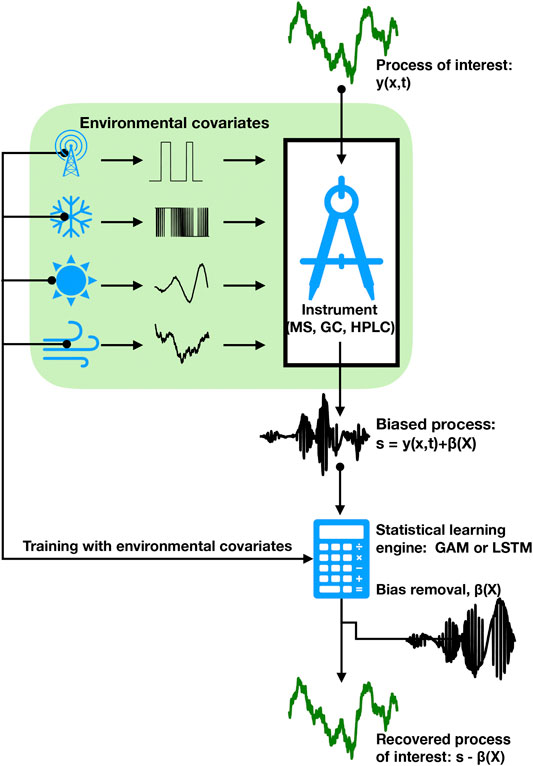
FIGURE 1. A schematic depiction of the effect of environmental factors on the introduction of bias into in situ chemical instrumentation and the subsequent identification and removal of bias using environmental covariates to train a statistical learning engine.

The signals of interest to this study are measurements of gases dissolved in water and seawater using field-portable quadrupole mass spectrometers (QMS). We present examples of the GAM and LSTM applied to data from a submersible wet inlet mass spectrometer (SWIMS) that was used to measure dissolved oxygen in the top 150 m of the Sargasso Sea and Gulf Stream, in the subtropical Atlantic Ocean. We present a second example of signals collected with a similar mass spectrometer aboard a ship that was used to measure dissolved carbon dioxide at the ocean surface, within the sea ice-covered Ross Sea, Antarctica.

Throughout this text, we make references to Python modules that were used to implement the individual solutions. The implementation of the GAM backfit algorithm, as well as example scripts for applying these methods to SWIMS data, can be found in the Supplementary Material and in the Acknowledgments.

Methods

The bias correction models were each applied to ocean measurements of gases dissolved in seawater. These measurements were made using a QMS. The QMS is an ideal tool for ocean measurements because it is compact, and it can scan over a large range of atomic masses. In this study, we refer to the mass-to-charge ratio (m/z), where m represents the atomic mass of the molecule of interest, and z represents the positive charge state. For example, water vapor is measured in the QMS at m/z = 18, and molecular oxygen (O₂) is measured at m/z = 32. In this study, z = 1 in every instance. The QMS can be connected to a variety of gas inlet configurations. Further detail on the principles of quadrupole mass spectrometry can be found in Dawson and Herzog, 1995, but they are not needed to follow the methods presented here.

Ocean Data Used to Evaluate the Bias Correction Models

Submersible Wet Inlet Mass Spectrometer Tow

The first ocean dataset was collected in July 2017 along a dynamic section of the subtropical Atlantic between 35° and 40° N latitude (Figure 2). The QMS was incorporated into a submersible wet inlet mass spectrometer (SWIMS), which is capable of in situ gas analysis to a water depth of 2000 m; in this application, we towed the mass spectrometer through water depths from 0 to 150 m aboard a Triaxus tow vehicle, corresponding to a region where sunlight penetrates the surface ocean. The triaxus tow vehicle was also equipped with a CTD to measure water column properties. The SWIMS position can be visualized by the gray saw-tooth pattern in panel b of Figure 3. Calibration of the SWIMS instrument is described below in In Situ Calibration of the Submersible Wet Inlet Mass Spectrometer.

FIGURE 2

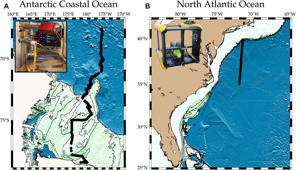
FIGURE 2. Maps showing the ocean regions where QMS data were collected as part of oceanographic surveys. Panel (A) is a region in the Ross Sea, along the coast of Antarctica in the Atlantic sector; panel (B) shows a region of the North Atlantic, including the Gulf Stream and Labrador water. The measurements collected at these locations are the subjects of the additive model and neural network bias correction algorithms that we compare in this study.

FIGURE 3

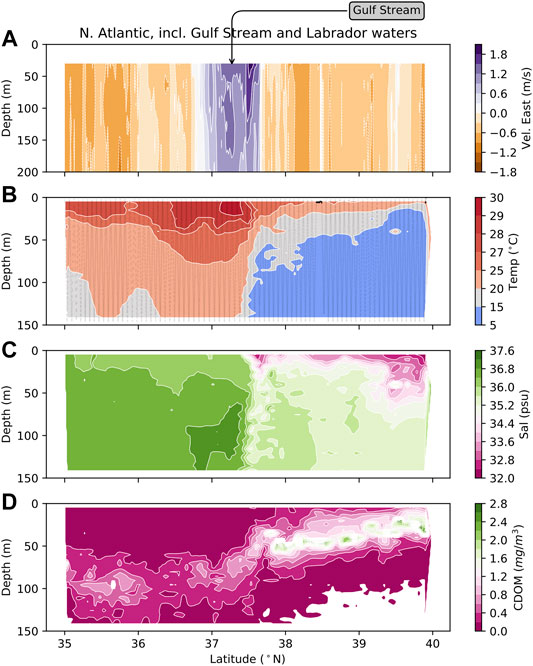
FIGURE 3. Ocean properties during the SWIMS tow in the N. Atlantic, across the Gulf Stream and into coastal waters influenced by the Labrador Current. The track lines of the tow are shown in panel (B).

This ocean section began in the North Atlantic subtropical gyre, a circulation feature that is known to be highly depleted of nutrients with low biomass (Jenkins, 1982). In summer, surface waters in the Gulf Stream and gyre can exceed 30°C, and nearly 1% of temperature measurements in this section fell between 30° and 35°C (Figure 3). North of the Gulf stream, waters cool and become significantly fresher, reflecting river inputs and the influence of the southward-flowing Labrador Current (Chapman and Beardsley, 1989). We chose to test the bias correction models in this region because the environment is highly changeable on a small horizontal and vertical scale; so, the SWIMS is subjected to a wide range of environmental conditions, including temperature, salinity, and dissolved organic matter—all of which can cause the dissolved gas burden of the seawater to vary.

The SWIMS was being used to measure oxygen, argon, carbon dioxide, nitrogen, and methane in the surface ocean. Each of these dissolved gases has significance for biology and geochemistry of the ocean. Our in situ calibration system included reference gases for each of these compounds, allowing the SWIMS to reproduce realistic concentration distributions for each analyte. Here, we will restrict analysis of the bias correction to the SWIMS signal at m/z = 32, corresponding to dissolved oxygen. By developing the bias correction at m/z = 32, we are able to take advantage of independent measures of dissolved oxygen using a membrane oxygen sensor, the Seabird model SBE 43, which allows for a detailed reference time series, throughout the vehicle tow. Ultimately, we use the root mean square error between the SBE43 and the SWIMS to establish a truly independent measure of the bias correction algorithm.

Shipboard Quadrupole Mass Spectrometers

The bias correction models were also tested on data from a shipboard QMS that continuously sampled dissolved gases in the Ross Sea sector of the South Atlantic, south of 75°S. These measurements were collected between May 16 and June 4, 2017. The partial pressure of carbon dioxide (pCO₂) was measured by connecting the QMS directly to a turbulent air-water equilibrator of the type described by Takahashi (1961). The same equilibrator was used to measure pCO₂ by infrared absorption spectroscopy (Takahashi et al., 2002; Takahashi et al., 2009); again, this provided an independent measurement to compare against the bias correction. The QMS was connected to the equilibrator with a 2 m × 50 μm (len × dia) capillary, which served to throttle the gas flow into the QMS and thereby maintain a vacuum below 10^–5 torr.

Carbon dioxide was measured with the QMS by scanning at the atomic mass m/z = 44. The reconstruction of pCO₂ was carried out with a daily 3-point linear calibration with reference gases of pCO₂ = 0%, 0.4%, and 0.1%. These signals can be seen in the expanded scale on the right side of Figure 4. Unlike the SWIMS tows, these calibrations were not long enough in duration to record the bias while sampling from a stable gas concentration. Therefore, we apply the bias correction to a time series of CO₂ partial pressure (pCO₂) measured at atomic mass m/z = 44. Instead, the GAM and LSTM models were trained on relatively stable ion current signals measured during a four-day period between May 27 and June 1.

FIGURE 4

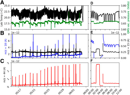
FIGURE 4. Time series of environmental correlates used to bias correct the pCO₂ signal measured by shipboard QMS at m/z = 44 (panels (C) and (F)). Panels (A) and (D) show the lab temperature and QMS vacuum pressure; panels (B) and (E) show water vapor (m/z = 18) and m/z = 15. Panels (D), (E), and (F) show the time series for one 12 h period on June 1, 2017.

This late autumn period in the Southern Hemisphere was cold and windy with continual disaggregated ice formation in the surface ocean. The principal source of bias appeared from the thermal cycling in the room where the QMS and equilibrator were operating (Figure 4). The heating system in that room would cause the temperature in the room to increase and decrease by 2-3°C every 30 min. Additionally, the seawater intake was periodically clogged with ice crystals, causing the equilibrator flow rate to vary.

In Situ Calibration of the SWIMS Instrument

The SWIMS passes seawater directly over a gas-permeable silicone membrane under conditions that approach a constant flow rate while maintaining constant water temperature using a resistive heater and aluminum block (Short et al., 2001; Wenner et al., 2004). The wet membrane inlet is a simple and elegant design that allows for a submersible instrument, but it is subjected to a number of confounding environmental influences that complicate interpretation of the SWIMS ion current. The most significant of these is a change in membrane permeability as it is compressed under the increasing water pressure (Bell et al., 2007). The permeability behavior is made more complex by hysteresis between the compression and decompression cycles (Futó and Degn, 1994; Lee et al., 2016). Over progressive cycles, the silicon membrane can become tempered and eventually exhibits less compressibility (Futó and Degn, 1994; Lee et al., 2016), which indicates that any bias correction should include multiple compression-decompression cycles to capture the longer term transients. To capture this and other sources of bias, we designed an in situ calibration method that involves connecting the SWIMS to a 1 L Tedlar bag that contains seawater, equilibrated with a reference gas mixture. The sample in the compressible Tedlar bag is subjected to the same pressure variations as the water column sample, but gas concentrations remain constant because there is no gas headspace in the bag. Using a 3-way solenoid switching valve, the SWIMS can change states from sampling the environment to sampling the constant reference gas. Because the gas concentration is invariant, any trends in ion current that are observed must be due to instrumental bias. An example of this instrumental bias can be observed in Figure 5, which shows the environmental correlates measured during approximately 4.8 tow cycles while measuring from the in situ calibration reference. These signal variations are what we seek to correct.

FIGURE 5

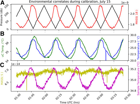
FIGURE 5. The six environmental correlates that were measured by the SWIMS instrument or CTD to capture variations in the environment that are likely to influence the signal response (s) of the SWIMS for m/z = 32 and other dissolved gases. Panel (A) shows instrument water depth as hydrostatic pressure and the ion current for water vapor (mass 18). Panel (B) shows the temperature of the electronics (uC temp) and the water temperature. Panel (C) shows the sample temperature or temperature of the heater block where gas is introduced across the membrane, and it shows ion current at mass 5, the electronic noise baseline.

Calibration after Bias Removal

To discover the instrument response, it is necessary to remove $\beta \left(X\right)$, the instrumental bias, and rearrange Eq. 1 as follows:

$y\left(\overrightarrow{x},t\right)=f(s-\beta \left(X\right)).(2)$

Here forward, we drop the explicit reference to uncorrelated error ($\mathit{\epsilon })$, which means that this error source is still a part of s. After bias correction, it is still necessary to estimate the uncertainty on y that is caused by $\mathit{\epsilon }$, but that topic is extensively covered by other studies, so it will not be addressed here.

Therefore, the steps to obtain y are to the first model $\beta \left(X\right)$, so that it can be removed, and then to calibrate to obtain the empirical dependency, $f\left(\right)$, between y and the bias-corrected signal. To make this procedure less abstract, we focus on measuring the oxygen concentration in seawater y = [O₂] using the ion current measured at m/z = 32. The raw ion current (s) in amps at m/z = 32 responds directly not only to the amount of O₂ dissolved in the water but also to other environmental correlates, X. The values of X must be measured as a time series, coincident with the instrument’s deployment. Other properties that we might include in X are, for example, the duty cycle of a heater or chiller, the atmospheric pressure, the temperature of a chemically reactive solute (e.g., pH-sensitive dye), or the electrical conductivity of a water solution. The environmental correlates used to model $\beta \left(X\right)$ in the SWIMS are shown in Figure 5, and the correlates used to model $\beta \left(X\right)$ in the shipboard QMS are shown in Figure 4.

After bias removal, $s$ reflects only the environmental signal of interest and some component of random error; $s_{-\beta }$ denotes the ion current after bias removal, and this term is calibrated against the reference gas concentrations using a linear equation,

$\begin{array}{l}f\left(s_{-\beta }\right)=m\left(s_{-\beta }\right)+b\text{or}\\ y\left(\overrightarrow{x},t\right)=m\left(s_{-\beta }\right)+s^0.\end{array}(3)$

Here, the terms m and $s^0$ are the slope and intercept, and these terms are estimated as described in Ocean Data Used to Evaluate the Bias Correction Models. Practically, we estimate m as

$m=\frac{y-y^0}{s_{-\beta }-s_{-\beta }^0}.(4)$

At the limit of $y^0$ = [O₂] = 0, the ion current does not reach zero because of electronic noise, and the potential for “virtual leaks” as gas is desorbed from the walls of the QMS under vacuum. In other words, $y^0$ is always zero, but in practice, $s_{-\beta }^0$ in Eq. 3 reflects the nonzero ion current at undetectable gas concentrations leaving the following linear calibration:

$y\left(\overrightarrow{x},t\right)=m\left(s_{-\beta }-s_{-\beta }^0\right).(5)$

The technique for determining $m$ and $s_{-\beta }^0$ for the shipboard QMS was determined by measuring m/z = 44 at pCO₂ = 0 in ultrapure N₂ gas, as described in Ocean Data Used to Evaluate the Bias Correction Models. The SWIMS determination of $m$ occurred during in situ calibration, which took place ca. every other day; however, we did not determine $s_{-\beta }^0$, so it became necessary to account for baseline drift in the SWIMS using an external reference. We implemented a reference to the equilibrium oxygen solubility, based on seawater temperature and salinity. We also used the SBE43 as a daily reference.

General Approach of Statistical Learning

The bias corrections that we evaluate here belong to a family of statistics called supervised learning. These corrections compare correlating inputs with corresponding outputs to develop a predictor that can be applied to any set of inputs. To develop the prediction, a sufficiently large dataset is divided into subsets—often referred to as “train” and “test” subsets (Ahmed et al., 2010). Separating in this manner allows the learning algorithm to develop a fit using the “train” dataset and evaluate the quality of that fit by predicting the data in the “test” dataset. The Scikit-learn module library in Python has been designed around the test-train convention and allows the user to subset using a number of different methods (Pedregosa et al., 2011). Last, the “test” dataset is used to estimate general error between the bias corrector and the actual data (Hastie et al., 2001).

Statistical learning models are exceedingly flexible and conform to almost any feature at any scale within a time series. This can result in “overfitting,” a condition where the learning algorithm attempts to reproduce small scale noise or other shapes in the data that do not improve the prediction or bias correction. Overfitting results because of the imperfect separation between the bias and the random error. This imperfect separation between $\beta$ and $\mathit{\epsilon }$, called the bias-variance tradeoff (Wood, 2017), results in a degradation of the fit as greater degrees of freedom are introduced to the model. Statistical learning algorithms included penalty parameters that can be adjusted to iteratively reduce the degrees of freedom. When this is done iteratively, one can probe the range of model-data misfit and determine the point where improved fitting becomes overfitting and then choose penalties accordingly in a process called regularization (Hastie et al., 2001). We describe the application of penalty regularization to the GAM in Implementation of the Generalized Additive Model and Backfit Algorithm and to the LSTM in Implementation of the Long Short-Term Memory Algorithm.

Implementation of the Generalized Additive Model and Backfit Algorithm

A GAM achieves smooth fitting by using the sum of fitting functions that individually represent the covariance between an individual input (X = p_i, q_i, r_i) and the response (y_i) data,

$y_i=y_0+f_1\left(p_i \right)+f_2\left(q_i \right)+f_3\left(r_i \right)+{\mathit{\epsilon }}_i.(6)$

The choice for fitting functions (f_j) is flexible, although a typical choice is a natural cubic spline. Natural cubic splines are a collection of polynomials, with second derivative equal to zero at the endpoints or knots. By specifying more knots, the splines can represent a higher frequency fluctuations. The fit between y and $f_1\left(p\right)$ can be generated through any penalized linear least-squares algorithm,

$\mathit{y}-{\text{f}}_{\text{j}}\left(\mathit{x}\right)+\lambda \underset{0}{\overset{1}{{\displaystyle \int }}}{\left[{{\text{f}}_j}^{″}\left(\mathit{x}\right)\right]}^{2}dx=0.(7)$

The fit penalization, $\lambda$, is the primary means by which the solution is tuned. The fit between y and the sum of f_j’s means that the influence of each f_j on the global solution can be observed, plotted, and evaluated. As mentioned, this is one of the principal strengths of the GAM, and it permits a more interactive and nuanced approach to determining the significance of each input variable and the behavior of each f_j.

We implemented the penalized least squares using the ridge regression algorithm in the Scikit-learn library with a specified value for penalization and normalization of all input variables;

>> model = Ridge(alpha = λ, normalize = true).

The natural cubic spline matrix with k = 9 knots was implemented using the Patsy module.

>> basis = dmatrix(“cr(train, df=10)-1”, {“train”: X[j]}).

We incorporated this penalized regression into the global fit using the backfit algorithm (Wood, 2017), which permits an iterative approach to fitting where each environmental correlate, j, is fit against the partial residuals (e_p), or the difference between the signal response (s) and the spline fit to all inputs except X_j,

$e_p^j=\widehat{s}-{\displaystyle \sum _{k\ne j}{f}_k\left(X_k \right)}.(8)$

Here, s has already been standardized or normalized to have zero mean. The backfit algorithm described by Wood (2017) has been reproduced here for clarity. The Python code can be found in the Supplementary Material.

Standardize or remove the mean from s: $\widehat{s}= s -\overline{s}$

Set the initial spline functions to zero: ${\mathbf{f}}_{\mathit{j}}=0$

Use linear regression to fit f_j to e_p: basis = model.fit(basis,e_p)

Estimate y from f_j: $\widehat{\text{s}}= {\displaystyle \sum }_j\widehat{{\text{f}}_j}$, news = basis.predict(dmatrix (“cr (valid, df = 10)-1”, {“valid”: X[j]})))

Recompute e_p: $e_p^j=\widehat{s}-{\displaystyle \sum }_{k\ne j}{\widehat{\text{f}}}_k\left(x_k \right)$

Repeat steps 3 thru 5 until e_p stops changing

More complex examples, involving other link functions between y and f_j and the imposition of different probability distributions on y_i (e.g., Gamma, Poisson or exponential), are all treated in more detail in Hastie et al. (2001).

To determine the optimal fit, we iteratively apply the backfit algorithm to the training data subset and then compute the generalized cross validation (GCV), as it varies with λ, the penalization parameter,

$V\left(\lambda \right)=\frac{\frac{1}{n}I-\mathit{A}\left(\lambda \right)y^2}{{\left[\frac{1}{n}tr\left(I-\mathit{A}\left(\lambda \right)\right)\right]}^2}.(9)$

In Eq. 9, n is the number of records of instrument signal response, I is the identity matrix, and A is the “influence” matrix, reflecting the penalized linear least-squares solution that can be applied as a step during the GAM fit (Golub et al., 1979),

$\mathit{A}\left(\lambda \right)=\mathit{X}{\left( {\mathit{X}}^T\mathit{X}+n\lambda I\right)}^{-1}{\mathit{X}}^T.(10)$

The GCV approach is to look for the minimum in $V\left(\lambda \right)$ to determine the most appropriate regularization penalty and strike the best balance between fit complexity and overfit. The GCV metric is better suited for this task than seeking the minimum residual sum of squares because that value decreases continuously with n and with the magnitude of $\lambda$.

The GCV score can be computed directly using Eq. 9. It is also computed and can be output by the Scikit-learn regression() toolbox. We used ridge regression, and the GCV score is output as >> model = Ridge (alphas = λ, store_cv_values = True).fit(X_train, s_train).

>> gcv = model.score (X_test, s_test).

Because the components of the GAM model are separable, it is also possible to determine which environmental correlates contribute most to the best-fit solution. This avoids the inclusion of correlates that make no contribution or may even degrade the GAM solution. The Bayesian information criterion (BIC) considers the model fit quality but also penalizes for models of increasing complexity (Burnham and Anderson, 2004), providing a measure for each correlate’s contribution to the GAM solution,

$BIC=n {\text{log}}_e\left(RSS/n\right)+k{\text{log}}_e\left(n\right).(11)$

This version of the BIC applies when using a maximum likelihood estimator (such as ridge regression). The term k is the number of parameters included in the model. In this case, k is equivalent to the number of environmental correlates. The absolute value of BIC is not important; rather, the goal is to seek a minimum in BIC, which indicates the model best fit with the fewest parameters. For this task,

$\Delta BI{C}_i=BI{C}_i-\text{min}\left(\text{BIC}\right)(12)$

will achieve a value of zero when the best set of environmental correlates have been used. The $\text{Δ}BIC$ is further useful as it allows the user to determine if certain environmental correlates degrade the overall solution or make no contribution (Figure 6).

FIGURE 6

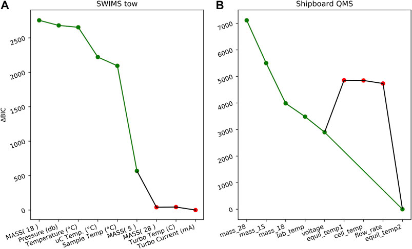
FIGURE 6. The normalized Bayesian information criterion ($\Delta BIC$) which was used to determine the set of the environmental correlates that best reproduce the bias in the GAM model. The black line with red dots indicates environmental correlates that did not measurably improve the $\Delta BIC$ score. These were left out of the final set of environmental correlates, which are indicated by the green line and green dots.

Implementation of the Long Short-Term Memory Algorithm

Recurrent neural networks (RNN) can be used to interpret sequential data, like time series, where each data record may be related to the records that preceded it. The neural network uses functional dependencies along a network of nodes, and the influence of these dependencies is weighted based on their relative importance. The RNN keeps track of these network weights as a means to archive predictive information as memory (Brownlee, 2019b). Since their development, RNNs sometimes have difficulty converging to a solution when attempting to optimize weights at all the nodes. This problem was solved by the LSTM algorithm (Hochreiter and Schmidhuber, 1997) that discards or “forgets” weight information that is not pertinent to the solution. The documentation of RNN theory, concepts, and implementation is very extensive, rapidly evolving, and available in the public domain, so we will move straight to a discussion of the implementation for instrument bias correction. We used the Keras API (Chollet, 2018) which serves as an interface to the TensorFlow toolbox to develop, train, and implement the LSTM network.

Taxonomy of the Time Series Forecast

Because there are so many types of problems that can be solved using neural networks, it is helpful to list out the characteristics of this particular time series solution because this affects the structure of the neural network (Brownlee, 2019b). In our case, we are determining a single output from multivariate inputs; the neural network is a regression, rather than classification; we seek a multitime step output to be able to predict over an unspecified range of time, and the current solution is static because it has been trained using in situ calibration data and does not update the solution over time. The exogenous inputs are water temperature and water hydrostatic pressure that the SWIMS experiences. The endogenous inputs, which are coinfluenced by the environment are water vapor inside the SWIMS detector, measured at m/z = 18, the sample temperature, the circuit board temperature, and the mass spectrometer background noise measured at m/z = 5 (Figure 4).

Instrument bias correction can be thought of as time series prediction. Even though our approach is to use a multivariate set of inputs to help develop the bias prediction, the potential for long-term transients in the instrument signal encourage the interpretation of bias correction as a sequential and time-dependent statistical problem. Examples of instrumental memory can include, e.g., the silicon membrane stiffening (In Situ Calibration of the Submersible Wet Inlet Mass Spectrometer) or the thermal inertia, a pressure casing that may dampen the heat transfer between the environment and electronics inside the housing.

We use the Keras sequential() model. The 2D environmental array X of n data records through time by k input parameters (e.g., temperature and pressure) must be reshaped into a 3D array or tensor. The n data records in time are decomposed into p sequences of t time steps: $n=p\times t$ (Stevens and Antiga, 2019). Tensor creation provides the RNN with multiple time series realizations against which to train and develop network weights. The fundamental choice for the user is to decide how many t time steps to include in each sequence. If data are periodic, it may be instructive to break the data into lengths that roughly capture an interval of the period. For example, two years of solar radiation data or sea level data measured every 10 min may be naturally broken into t = 144 or t = 36 time steps corresponding to the 1-day or one half tidal period. However, this choice is rarely carried out a priori and must be determined iteratively.

After the $p\times t\times k$ tensor dimensions have been established, the user must choose a functional relationship or “activation function” between input and response at each network node, the number of iterations or “epochs” over which the RNN algorithm will train, and the number of “neurons” and the “optimizer” or metric that is used to evaluate the goodness of fit. As with the time steps, the settings for these parameters cannot be determined a priori, so we establish appropriate values through iteration (Brownlee, 2019b).

Keras allows a user to take control of when the RNN weights are updated; this is known as controlling the model state or “stateful = True.” By default, Keras updates the LSTM state after a “batch” is processed. A batch is a collection of sample sequences, where each sample sequence has t timesteps, as we defined above. A batch size of one causes the model weights to be updated after each sample, but the penalty in processing speed and computation often requires a large batch size. Ideally, the batch size is a factor of p, the number of sample sequences; otherwise, a set of left over sequences are processed in an additional step (Brownlee, 2019b).

Determining Fit Quality

During tuning and iteration of the GAM model, we used GCV($\lambda$) to test for overfitting and the root mean square error (RMSE), which is a measure of the deviation between modeled bias $\widehat{\beta }\left(X\right)$ and instrument bias, using the train datasets. We also evaluated the neural network LSTM model using the RMSE between $\widehat{\beta }\left(X\right)$ and the instrument bias, measured during in situ calibrations.

To evaluate the overall fit quality, we measured the RMSE between the independent O₂ and CO₂ instruments (y_ind), and the bias-corrected signal from the QMS and SWIMS instruments as defined by Eq. 5, ($y\left(\overrightarrow{x},t\right)$):

$RMSE= \sqrt{\frac{1}{n}{\left(y\left(\overrightarrow{x},t\right)-y_{ind}\right)}^2}.(13)$

Results and Discussion

The bias correction workflow is depicted in Figures 1and7; the calibrated GAM solution is shown in Figure 7 panels b through d, but the steps are essentially the same for the LSTM solution. In this section, we present the details of the GAM and LSTM fits and contrast the two bias correction models.

FIGURE 7

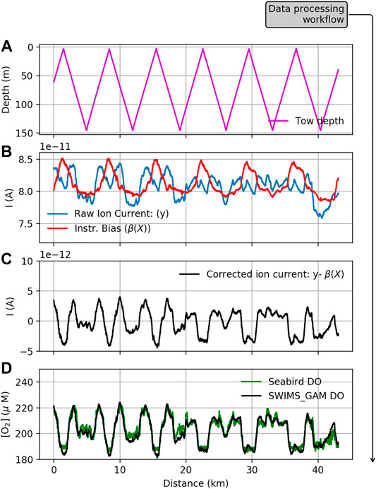
FIGURE 7. Sequence showing the SWIMS tow and bias correction using the generalized additive model (GAM). Panel (A) reveals the depth recorded by the Triaxus CTD during vertical tows; panel (B) shows the raw signal recorded for oxygen at m/z = 32 and the estimate of instrumental bias. Panel (C) shows the corrected ion current, and panel (D) shows the calibrated ion current in O₂ concentration units, alongside the Seabird DO sensor.

Generalized Additive Model Fit

The ability to choose a functional form for each X_j environmental correlate was an attractive feature of the GAM because early tests revealed that oxygen (m/z = 32) strongly correlated with water vapor (m/z = 18), and signal from the SWIMS showed m/z = 18 ion currents outside the range observed during in situ calibration. Consequently, it appeared necessary to have a linear or proportional correction to m/z = 18. Water is present in solution at nearly 1 mol/mol; so, its concentration far exceeds the other analytes. Somewhat counterintuitively, m/z = 18 correlated positively with m/z = 32, perhaps suggesting a similar response to membrane permeability rather than competition for ionization inside the SWIMS source (Supplementary Figure S1).

All the environmental correlates (Figure 5) negatively covaried with the water depth. More subtle features, such as lag between the circuit board temperature (uC temp) and the sample temperature can also be observed in the SWIMS electronics temperature (Figure 5, panel b). Using the flexibility of the GAM, we tested both linear and quadratic fits between m/z = 18 and the target output variable [O₂] or m/z = 32. While these parameterizations showed a stiffer, more proportional response to the large-scale variations in m/z = 18; ultimately, the natural cubic spline produced the best RMSE solution.

Having chosen a cubic spline functional form for f() for each X_i, there remain only two additional parameters that can be used to tune the solution—the number of knots in each spline and the value of the penalty function, λ (Eq. 9). We tested the fit to in situ calibration data for a range from 3 to 30 knots and observed no significant change in fit quality above 10 knots, so all cubic spline fits used a total of 10 knots. The term GCV(λ) was computed iteratively over a range from λ = 10^–10 to λ = 10¹⁰ (Figure 8); the minimum GCV(λ) suggests the region where fit complexity and minimization of bias are optimal (Wood, 2017). We found GCV(λ) was not sensitive to the penalty, outside the range 10^–2 < λ < 10⁵, with a minimum near λ = 10⁵, so this value of the penalty was implemented in the solution.

FIGURE 8

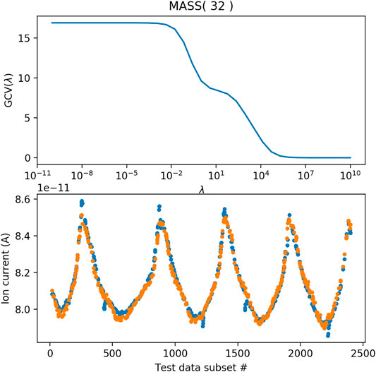
FIGURE 8. Test of the GAM solution using a range of values for the penalty term λ in Eq. 9. Orange circles represent the GAM reconstruction and blue circles represent the raw ion current during in-situ calibration.

Long Short-Term Memory Fit

As noted, the Keras LSTM algorithm requires iteration to choose appropriate values for the t time steps in each sample, the batch size, and epochs, as well as the choice for how often to update the weights of the RNN or statefulness. We chose to optimize based on the RMSE and used a hyperbolic tangent activation function. We found the LSTM solution was most sensitive to batch size and the number of epochs, especially as they related to overfitting. To mitigate overfitting, we implemented node dropout regularization using the Keras dropout() attribute. The approach is to assign a dropout likelihood between 0 and 1, wherein the model will randomly remove some nodes during training, thereby reducing codependence and overweighting of certain nodes (Srivastava et al., 2014).

Because the choice of batch_size, epoch number, and dropout regularization cannot be determined a priori, but have a preponderant influence on overfitting, we objectively determined the optimal values for these three hyper parameters using the GridSearchCV() algorithm in Keras. The approach tries all permutations of the hyper parameters and measures the fit quality using the RMSE and a k-fold cross validation (with k = 5). The k-fold cross validation randomly samples the training data to produce test data subsets, which are then used to measure fit quality k times. We tested batch_sizes ranging from 20 to 80, epoch numbers ranging from 5 to 30, and dropout likelihood ranging from 0.1 to 0.8. The smallest k-fold RMSE value was found at with a batch_size = 80, epochs = 20, and dropouts = 0.4. The residual error between the training data and the LSTM solution, “train RMSE” in Figure 9, reveals a continual reduction in both test and train RMSE through epoch = 20. Beyond epoch = 20, the test RMSE increases, suggesting an overfit (Figure 9).

FIGURE 9

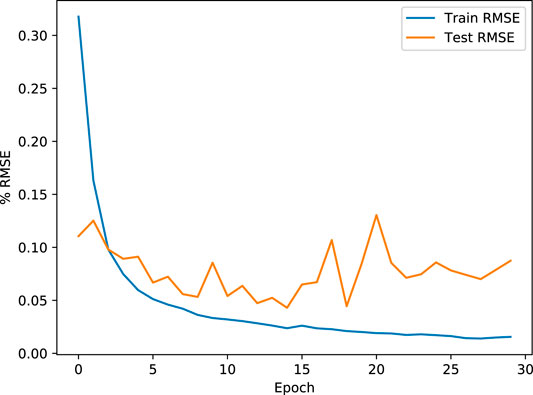
FIGURE 9. Root mean squared deviation between the train and test subsets during successive training epochs. While the training RMSE continually decreases, suggesting improvement, the test RMSE begins to increase after 20 epochs, suggesting that the solution is being overfit.

Finally, the choice of t timesteps in each sample can be an important consideration. Because time series may have quasiperiodic correlations, it is desirable to have t be large enough to capture the full period, in order to make future predictions based on past time series behavior (Brownlee, 2019a). The Triaxus tow vehicle was programmed to ascend and descend at 0.2 m/s, so a full tow from surface to 150 m and back to the surface took approximately 25 min or t = 750 time steps at data reported every 2 s, which is the scan rate of the SWIMS. Initially, we anticipated that a sample size of t > 750 would provide the best fit. However, splitting the in situ calibration data into a test and train subset did not permit the inclusion of sample sizes of t = 750 because we felt it is necessary to validate against a test dataset that was at least 2 t in length. In practice, we tested values of t = 50, 100, 200, and 300. The test RMSE actually improved significantly as t was reduced. Eventually, t = 100 provided both computational efficiency and low RMSE, even though this number of time steps does not encompass the full profile tow. The tow profile may not be as necessary, suggesting that the information used to reconstruct the bias comes from the environmental correlates that are available at the prediction timestep, rather than from the learned temporal dependence.

GAM vs. LSTM Bias Correction, SWIMS Tow

Normally, the procedure to evaluate a statistical learning algorithm involves validating the solution against the test data (General Approach of Statistical Learning), which was set aside before the training stage. However, the independent measurement of oxygen by the SBE43 (Ocean Data Used to Evaluate the Bias Correction Models) provides an opportunity to quantify the bias correction against an entirely unique measure of oxygen. It should be noted that the SBE43 probe can also be subject to its own sources of bias, some of which may not be accounted for, but this instrument has a long performance history in oceanography (e.g., Helm et al., 2011) that supports the choice to use it as a reference instrument.

The final list of environmental correlates was determined using the $\text{Δ}BIC$ metric (Eq. 12). In addition to water vapor, we tested for environmental covariation in the water pressure, seawater temperature, the sample temperature inside the SWIMS heater block, the circuit board temperature, the temperature of the turbo pump, current draw of the turbo pump, and the duty cycle of the membrane heater. Using $\text{Δ}BIC$, it was determined that these last parameters did not add any meaningful additional constraints beyond what the first six environmental correlates. That is, $\text{Δ}BIC$ achieved a minimum after including water vapor, water pressure, circuit board temperature, sample temperature, and instrument noise at m/z = 5 (Figure 6). The remaining correlates were eliminated from the GAM solution.

The SWIMS tow between 35° and 40° N recorded a total of N = 49,181 individual measurements of dissolved O₂. A contour plot of dissolved O₂ reveals the tracer field in Figure 10. The RMSE between SBE43 and bias-corrected SWIMS data using the GAM was 11.2 µM (micromoles per liter of seawater); the units of RMSE are the same as the concentration data itself. The mean [O₂] in this section was 196 µM, suggesting a 5.7% deviation between the two instruments. Within the same section, the neural network LSTM bias correction yielded RMSE = 9.8 µM or 5.0% deviation overall. Both GAM and LSTM bias corrections tended to fit some regions better than others; however, the fit quality of the GAM and fit quality of the LSTM did not degrade in the same places, suggesting some differences in how the two models respond to the environmental correlates (Figure 5).

FIGURE 10

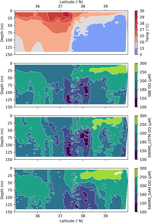
FIGURE 10. North Atlantic section, including Gulf Stream and Labrador waters showing temperature (top) and oxygen from the Seabird SBE 43 membrane and the SWIMS with bias corrections using GAMs and the neural network LSTM model.

It should be noted that we are focusing on interpretation of the relative RMSE between the GAM and LSTM solutions. The absolute value of the RMSE is less meaningful because the calibration intercept ($s^0$) was not measured on the SWIMS in-situ calibrations. This term, $s^0$, represents the instrument baseline drift, and so, we determined $s^0$ by optimal fit to the SBE43. The same baseline drift can be determined by fitting to another independent reference, such as the equilibrium oxygen solubility (Garcia and Gordon, 1992). When we use equilibrium solubility, the shape or trend in the daily estimates of $s^0$ remains the same, but the magnitude of $s^0$ shifts, causing a larger misfit between the SBE43 and the SWIMS. During future in situ calibrations, we think it is possible to implement a workable measure of $s^0$ by shutting off the water pump, causing all the gas around the silicon membrane to be depleted and achieving a practical value of zero concentration for all gases except water vapor.

GAM vs. LSTM Bias Correction, Shipboard Quadrupole Mass Spectrometers

The bias corrections in the shipboard QMS were fit using training data over a four-day period of the surface ocean equilibrator time series from May 27 to June 1. The RMSE between the GAM solution and training data subset was 3.5%, and the LSTM misfit was 1.8%. Unlike the SWIMS tows, it was not possible to evaluate $\beta \left(X\right)$ independent of the environmental signal $y(\overrightarrow{x},t)$. The daily calibrations with reference gases did not take place for long enough to properly observe and decompose the time series aliasing. Instead, it was necessary to train the LSTM and GAM models on a section of the real-time series. This approach can lead to muddling the separation between $y\left(\overrightarrow{x},t\right)$ and $\beta \left(X\right)$, potentially correcting away some of the environmental signals in pCO₂ during the bias correction. However, the ambient changes in pCO₂ should reflect the biology and chemistry which in turn are only partly dependent on the exogenous environmental correlates. The endogenous environmental correlates reflect instrument behavior, which should have zero correlation with environmental pCO₂. The environmental correlates used to develop the bias correction model included, 1) temperature of the lab where the QMS was installed, 2) the total gas pressure in the QMS measured as voltage, 3) the seawater flow rate through the turbulent equilibrator, 4) water vapor measured at m/z = 18, and 5) m/z = 15. Similar to the SWIMS tow, we found that three environmental correlates caused an increase (no decrease) in $\text{Δ}BIC$ metric, signaling that they contributed no meaningful constraint. Consequently, the IR pCO₂ cell temperature, the water wall flow rate, and the second equilibrator temperature reading were eliminated from the bias correction solutions (Figure 6).

After bias correction, the raw ion current was calibrated to CO₂ partial pressure, using the three-point calibration of reference standards that were measured daily. There are additional corrections to gas measurements that are made using a turbulent equilibrator, and these are described by Takahashi et al. (2009). These corrections have not been implemented here; while their implementation might improve the overall misfit between the two measurements of pCO₂, they would drop out of the comparison between GAM and LSTM bias corrections; so, these additional data corrections are not material to this evaluation.

In this case, the GAM model was better at removing the periodic oscillation in the QMS ion current at m/z = 44 (). However, a level of noise persists even after the bias correction, suggesting that the environmental correlates may be missing some components of the bias. In total, the 18-day time series contains 5043 unique measurements of pCO₂ by infrared absorption spectroscopy and by QMS. The RMSE between the IR pCO₂ and GAM-corrected pCO₂ was 31.3 μatm; the average pCO₂ was 411 μatm, revealing an overall misfit of 7.5% (Figure 11). The LSTM RMSE was 35.2 μatm or 8.5% of the mean pCO₂. In this case, it appears the LSTM (not pictured) may have slightly overfit the training data, resulting in a degraded fit to the overall time series. Nevertheless, the difference in RMSE between GAM and LSTM was less than 1%, which suggests that both methods produce very similar overall bias correction outcomes.

FIGURE 11

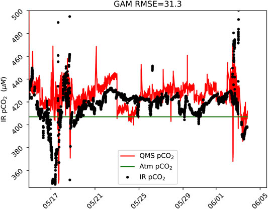
FIGURE 11. Bias-corrected and calibrated pCO₂ from shipboard QMS alongside measurements of pCO₂ by infrared absorption spectroscopy (IR pCO₂) in the Ross Sea, 2017.

Summary

This study presents two models for instrument bias correction, a GAM and a LSTM neural network model. The two models represent philosophically different approaches to the multivariate prediction; the GAM allows the user to investigate the intermediate model fit products and choose the functional form f() for optimal regression between the results and the individual environmental correlates in X. This advantage was particularly useful when interrogating which environmental influences to include as correlates in the model solution, using the $BIC$ criterion. This calculation is straightforward and can be determined offline without iteration of the GAM model, precisely because the solution is separable. The procedure eliminated three environmental correlates from both Shipboard and SWIMS ocean datasets (Figure 6). The six remaining correlates were also used to fit the LSTM solution.

The LSTM RNN model gives the user fewer intermediate diagnostics, which produces an initial lack of confidence in the robustness of the solution because it can be challenging to understand or visualize the nature of the solution. Nevertheless, there is an emerging recognition that, compared to the human brain, computers are much more capable instruments at assigning appropriate weights to an n-dimensional set of variates in pursuit of a solution. By accepting these models, we implicitly acknowledge that the multivariate weights in the solution are beyond our capacity to evaluate simultaneously, thus rendering the “black box” criticism somewhat moot. However, the procedures for implementing RNNs, including the grid search or random search (B. Nakisa et al., 2018; Bergstra and Bengio, 2012), provide a systematic approach to determining the optimal tuning of hyperparameters (e.g., times steps, batch size, epochs, and hidden nodes), and the eventual robustness of the solution has held up under rigorous testing and comparison. In the SWIMS dataset with in situ calibration, the LSTM solution proved more effective at removing bias in the high gradient oceanic region, with tows across the Gulf Stream. However, the GAM exhibited better fit quality in the Antarctic shipboard QMS dataset, as compared to the LSTM.

The difference between GAM and LSTM RMSE was 1% or less for both ocean sections, suggesting that both models performed similarly well. The RMSE for both methods were better than 6% for O₂ and less than 9% for CO₂, demonstrating a predictive accuracy of better than 91% for both dissolved gases. The quality of the bias removal solution was significantly more dependent on the availability of coincidently sampled environmental correlates as inputs. We further found that the in situ calibration for SWIMS data was a significant factor in producing a high fidelity bias correction. Several attempts were made to produce the same bias correction using just SWIMS tow data (without the in situ calibration) as training data, and the solution was significantly diminished with an RMSE for the LSTM model of 17% as compared to 5% with the in situ calibration. These results demonstrate that the bias corrections are most effective when they can be tuned using the in situ calibration with an invariant reference gas to reveal the instrument bias.

The overall performance of the GAM and LSTM models was highly comparable, making it difficult to declare a clear winner in this case. The primary advantage conferred by the GAM model is the ability to evaluate the fit to each individual correlate, separately. This is a big advantage when it is necessary to better understand an instruments behavior and might even lead to engineering solutions that eliminate the biggest source of bias. In comparison, the skill that an LSTM RNN brings to time series prediction can potentially serve to model longer-term transients in the signal, which could lead to a better bias model when few or no environmental correlates been measured.

Data Availability Statement

The entire workflow including code, writeup, and source data with BCO-DMO DOI can be found at https://github.com/bloose/bias_correction_by_ML/.

Author Contributions

BL developed and tested the bias correction methods described here, and lead the field data collection program. RT Short co-developed the SWIMS instrument and in-situ calibration system, and participated in the field data collection. ST participated in the field data collection.

Funding

This work was supported by a grant from the National Science Foundation, Award # 1429940.

Conflict of Interest

The authors declare that the research was conducted in the absence of any commercial or financial relationships that could be construed as a potential conflict of interest.

Acknowledgments

This research was supported by an award from the National Science Foundation Chemical and Biological Oceanography Program #1429940. We thank two anonymous reviewers for the comments and suggestions that have improved this manuscript. The GAM backfit algorithm is available at https://github.com/bloose/Python_GAM_Backfit. The supplemental contains annotated Python scripts and SWIMS example data to demonstrate application of the GAM and LSTM to bias correction.

Supplementary Materials

The Supplementary Material for this article can be found online at: https://www.frontiersin.org/articles/10.3389/feart.2020.537028/full#supplementary-material

References

Ahmed, N. K., Atiya, A. F., Gayar, N. E., and El-Shishiny, H. (2010). An empirical comparison of machine learning models for time series forecasting. Econom. Rev. 29, 594–621. doi:10.1080/07474938.2010.481556

CrossRef Full Text | Google Scholar

Bell, R. J., Short, R. T., van Amerom, F. H. W., and Byrne, R. H. (2007). Calibration of an in situ membrane inlet mass spectrometer for measurements of dissolved gases and volatile organics in seawater. Environ. Sci. Technol. 41, 8123–8128. doi:10.1021/es070905d

CrossRef Full Text | Google Scholar

Bergstra, J., and Bengio, Y. (2012). Random search for hyper-parameter optimization. J. Mach. Learn. Res. 13, 281–305.

Google Scholar

Brownlee, J. (2019a). Deep learning for time series forecasting: predict the future with MLPs, CNNs and LSTMs in Python (Jason Brownlee).

Google Scholar

Brownlee, J. (2019b). Long short-term memory networks with Python. Australia: Jason Brownlee.

Google Scholar

Burnham, K. P., and Anderson, D. R. (2004). Multimodel inference. Socio. Methods Res. 33, 261–304. doi:10.1177/0049124104268644

CrossRef Full Text | Google Scholar

Cassar, N., Barnett, B. A., Bender, M. L., Kaiser, J., Hamme, R. C., and Tilbrook, B. (2009). Continuous high-frequency dissolved O2/Ar measurements by equilibrator inlet mass spectrometry. Anal. Chem. 81, 1855–1864. doi:10.1021/ac802300u

CrossRef Full Text | Google Scholar

Chapman, D. C., and Beardsley, R. C. (1989). On the origin of shelf water in the middle atlantic bight. J. Phys. Oceanogr. 19, 384–391. doi:10.1175/1520-0485(1989)019<0384:otoosw>2.0.co;2

CrossRef Full Text | Google Scholar

Chollet, F. (2018). Deep learning with Python. Shelter Island, NY: Manning Publications.

Google Scholar

Dawson, P. H., and Herzog, R. F. (1995). Quadrupole mass spectrometry and its applications. New York, NY: American Institute of Physics.

Google Scholar

Delle Monache, L., Nipen, T., Deng, X., Zhou, Y., and Stull, R. (2006). Ozone ensemble forecasts: 2. A Kalman filter predictor bias correction. J. Geophys. Res. Atmospheres 111, D05308 doi:10.1029/2005jd006311

CrossRef Full Text | Google Scholar

Futó, I., and Degn, H. (1994). Effect of sample pressure on membrane inlet mass spectrometry. Anal. Chim. Acta 294, 177–184. doi:10.1016/0003-2670(94)80192-4

CrossRef Full Text | Google Scholar

Garcia, H. E., and Gordon, L. I. (1992). Oxygen solubility in seawater: better fitting equations. Limnol. Oceanogr. 37, 1307–1312. doi:10.4319/lo.1992.37.6.1307

CrossRef Full Text | Google Scholar

Golub, G. H., Heath, M., and Wahba, G. (1979). Generalized cross-validation as a method for choosing a good ridge parameter. Technometrics 21, 215–223. doi:10.1080/00401706.1979.10489751

CrossRef Full Text | Google Scholar

Guegen, C., and Tortell, P. D. (2008). High-resolution measurement of Southern Ocean CO2 and O2/Ar by membrane inlet mass spectrometry. Mar. Chem. 108, 184–194. doi:10.1016%2Fj.marchem.2007.11.007

CrossRef Full Text | Google Scholar

Hastie, T., Tibshirani, T., and Friedman, J. (2001). The elements of statistical learning: data mining, Inference, and prediction. Berlin: Springer.

Google Scholar

Helm, K. P., Bindoff, N. L., and Church, J. A. (2011). Observed decreases in oxygen content of the global ocean. Geophys. Res. Lett. 38, 23602. doi:10.1029/2011gl049513

CrossRef Full Text | Google Scholar

Hochreiter, S., and Schmidhuber, J. (1997). Long short-term memory. Neural Comput. 9, 1735–1780. doi:10.1162/neco.1997.9.8.1735

CrossRef Full Text | Google Scholar

Jenkins, W. J. (1982). Oxygen utilization rates in North Atlantic subtropical gyre and primary production in oligotrophic systems. Nature 300, 246–248. doi:10.1038/300246a0

CrossRef Full Text | Google Scholar

Lee, W. S., Yeo, K. S., Andriyana, A., Shee, Y. G., and Mahamd Adikan, F. R. (2016). Effect of cyclic compression and curing agent concentration on the stabilization of mechanical properties of PDMS elastomer. Mater. Des. 96, 470–475. doi:10.1016/j.matdes.2016.02.049

CrossRef Full Text | Google Scholar

Nakisa, B., Rastgoo, M. N., Rakotonirainy, A., Maire, F., and Chandran, V. (2018). Long Short term memory hyperparameter optimization for a neural network based emotion recognition framework. IEEE Access 6, 49325–49338. doi:10.1109/access.2018.2868361

CrossRef Full Text | Google Scholar

Newman, M. C. (1993). Regression analysis of log-transformed data: statistical bias and its correction. Environ. Toxicol. Chem. 12, 1129–1133. doi:10.1002/etc.5620120618

CrossRef Full Text | Google Scholar

Pedregosa, F., Varoquaux, G., Gramfort, A., Michel, V., Thirion, B., Grisel, O., et al. (2011). Scikit-learn: machine learning in Python. J. Mach. Learn. Res. 12, 2825–2830.

Google Scholar

Pimentel, K. D. (1975). Toward a mathematical theory of environmental monitoring: the infrequent sampling problem. Dissertation. CA, United States: California University.

Google Scholar

Saltzman, E. S., De Bruyn, W. J., Lawler, M. J., Marandino, C. A., and McCormick, C. A. (2009). A chemical ionization mass spectrometer for continuous underway shipboard analysis of dimethylsulfide in near-surface seawater. Ocean Sci. 5, 537–546. doi:10.5194/os-5-537-2009

CrossRef Full Text | Google Scholar

Short, R. T., Fries, D. P., Kerr, M. L., Lembke, C. E., Toler, S. K., Wenner, P. G., et al. (2001). Underwater mass spectrometers for in situ chemical analysis of the hydrosphere. J. Am. Soc. Mass Spectrom. 12, 676–682. doi:10.1016/s1044-0305(01)00246-x

CrossRef Full Text | Google Scholar

Srivastava, N., Hinton, G., Krizhevsky, A., Sutskever, I., and Salakhutdinov, R. (2014). Dropout: a simple way to prevent neural networks from overfitting. J. Mach. Learn. Res. 15, 1929–1958.

Google Scholar

Stevens, E., and Antiga, L. (2019). Deep learning with PyTorch. Shelter Island, NY: Manning Publications.

Google Scholar

Sun, F., Xiong, R., and He, H. (2016). A systematic state-of-charge estimation framework for multi-cell battery pack in electric vehicles using bias correction technique. Appl. Energy 162, 1399–1409. doi:10.1016/j.apenergy.2014.12.021

CrossRef Full Text | Google Scholar

Takahashi, T. (1961). Carbon dioxide in the atmosphere and in Atlantic Ocean water. J. Geophys. Res. 66, 477–494. doi:10.1029/jz066i002p00477

CrossRef Full Text | Google Scholar

Takahashi, T., Sutherland, S. C., Sweeney, C., Poisson, A., Metzl, N., Tilbrook, B., et al. (2002). Global sea-air CO2 flux based on climatological surface ocean pCO2, and seasonal biological and temperature effects. Deep Sea Res. Part II Top. Stud. Oceanogr. 49, 1601–1622. doi:10.1016/s0967-0645(02)00003-6

CrossRef Full Text | Google Scholar

Takahashi, T., Sutherland, S. C., Wanninkhof, R., Sweeney, C., Feely, R. A., Chipman, D. W., et al. (2009). Climatological mean and decadal change in surface ocean pCO2, and net sea-air CO2 flux over the global oceans. Deep Sea Res. Part II Top. Stud. Oceanogr. 56, 554–577. doi:10.1016/j.dsr2.2008.12.009

CrossRef Full Text | Google Scholar

Wenner, P. G., Bell, R. J., van Amerom, F. H. W., Toler, S. K., Edkins, J. E., Hall, M. L., et al. (2004). Environmental chemical mapping using an underwater mass spectrometer. TrAC. Trends Anal. Chem. 23, 288–295. doi:10.1016/s0165-9936(04)00404-2

CrossRef Full Text | Google Scholar

Wood, S. (2017). Generalized additive models: an introduction with R. United States: CRC Press.

Google Scholar