Stochastic Simulation of the Spatial Heterogeneity of Deltaic Hydrofacies Accounting for the Uncertainty of Facies Proportions

The spatial geological heterogeneity of an aquifer significantly affects groundwater storage, flow and the transport of solutes. In the particular case of coastal aquifers, spatial geological heterogeneity is also a major determining factor of the spatio-temporal patterns of water quality (salinity) due to seawater intrusion. While the hydraulics of coastal hydrogeology can be modeled effectively by various density flow equations, the aquifer geology is highly uncertain. A stochastic solution to the problem is to generate numerical realisations of the geology using sequential stratigraphy, geophysical models or geostatistical approaches. The geostatistical methods (two-point geostatistics, Markov chain models and multiple-point geostatistics) have the advantage of minimal data requirements, e.g., when the only data available are from cores from a few sparsely located boreholes. We provide an extension of sequential indicator simulation by including the uncertainty of the hydrofacies proportions in the simulation approach. We also deal with the problem of variogram estimation from sparse boreholes and we discuss the implicit transition probabilities and the connectivity of simulated realisations of a number of categorical variables. The variogram model used in the simulation of hydrofacies significantly influences the degree of connectivity of the hydrofacies in the simulated model. The choice of model is critical as connectivity determines the amount and extent of seawater intrusion and hence the environmental risk. The methodology is illustrated with a case study of the Andarax river delta, a coastal aquifer in south-eastern Spain. This is a semi-arid Mediterranean region in which the increasing use of, and demand for, groundwater is exacerbated by a transient tourist population that reaches its peak in the summer when the demand for the permanent population is at its highest. The work reported here provides a sound basis for designing flow simulation models for the optimal management of groundwater resources. This paper is an extended version of a presentation given at the 2012 GeoENV Conference held in Valencia, Spain.

Introduction

Half of the world’s population lives in coastal areas and the transient and permanent populations of these areas continue to increase. This generates increasing, and often competing, demands for water. To meet demand, or allocate limited supply, and satisfy environmental and sustainability constraints in these coastal zones requires optimal management of water resources in general and groundwater resources in particular. The problem is exacerbated in the Mediterranean region because of the combined effects of semi-arid climate (high evapotranspiration and low rainfall) and seasonal tourism that increases the demand for water during the summer, which is the period of lowest aquifer recharge. The result is increased depletion of groundwater with the risk of over-extraction.

In coastal areas, over-extraction not only depletes the aquifer but also causes seawater intrusion leading to deterioration of water quality that may ultimately render the aquifer water unfit for human consumption and other uses such as agriculture. In general, mathematical models of aquifers comprise two parts: the medium (the geological materials that comprise the aquifer) and the passage of water (hydraulics) through the geological medium. The hydraulics are modeled effectively by various density flow equations but the geology, particularly the spatial distribution of the hydrofacies, introduces a major source of variability and uncertainty in any model or assessment of an aquifer. In general, the geology is heterogeneous and is unknown apart from limited direct data from sparse boreholes or the indirect geophysical information. Apart from borehole cores, the aquifer is not observable on any meaningful scale and the only realistic approach in such cases is via a stochastic model informed by sparse data and/or surface analogues (outcrops). The prediction of seawater intrusion is thus a stochastic problem.

The spatio-temporal patterns of groundwater quality in coastal aquifers are determined by the spatial heterogeneity and spatial distribution of hydrofacies (Eaton, 2006) as well as by different hydrologic settings and forcings. A general way to address the stochastic seawater intrusion problem is to accommodate the stochastic character of the geology by generating stochastic simulations of aquifer heterogeneity.

Although the techniques discussed here are generally applicable to different sedimentary environments, the focus in this paper is on deltaic environments. The three most common means of generating three-dimensional geological models (in this case, 3D models of hydrofacies) of deltas are sequential stratigraphy (Cabello et al., 2007), geophysical methods (Tercier et al., 2000; Deidda et al., 2006; Barakat, 2010) and geostatistical techniques (dell’Arciprete et al., 2012; Perulero et al., 1997). A good overview of statistical grid-based sedimentary facies reconstruction and modeling methods can be found in Falivene et al. (2007).

In an ideal situation, all of these techniques could be used to integrate all available information to generate a model that is as realistic as possible. However, the amount, type and quality of the available data constrain the choice of method. Of the three methodologies, geostatistical methods are the least demanding in terms of data requirements because they are based on the estimated underlying structural model and its uncertainty (Pardo-Igúzquiza et al., 2009) and they can be applied even when only a few sparsely located boreholes are available.

The geostatistical methods can be classified either as object-based methods (Gouw, 2007) or models based on pixels and voxels (Dubrule and Damsleth, 2001). The latter are the more flexible and, in turn, they can be classified as two-point geostatistical models (Deutsch and Journel, 1998), Markov chain models (Carle and Fogg, 1996) or multiple-point geostatistical models (Strebelle, 2002; Comunian et al., 2011). Multiple-point geostatistical methods require detailed three-dimensional training images, which are not usually available for groundwater applications although other sources such as surface analogues (e.g., Comunian et al., 2011), outcrops, geophysical images, outputs of numerical models can be used. Markov chain models tend to give simulations that are less realistic than the other methods; in particular, the hydrofacies are often too disconnected. For these reasons, we have chosen to use basic, second-order stationary geostatistical models and, in the work presented here, we have used sequential indicator simulation to generate realisations of categorical variables (Goovaerts, 1997). We also considered using truncated pluri-gaussian simulation (Le Loc’h et al., 1994; Le Loc’h and Galli, 1996; Dowd et al., 2003; Mariethoz et al., 2009) but decided against it because of the inability to infer facies contact relationships with an acceptable level of accuracy from cores from sparse boreholes. This method is more suitable for cases in which there are reliable surface analogues from which detailed contacts can be observed. A comparison of geostatistical methods for hydrofacies simulation is given in dell’Arciprete et al. (2012). The work presented here differs from the latter, which simulates alluvial sediments using vertical facies maps of five almost orthogonal quarry faces and no borehole data whereas we simulate deltaic sediments in a flat area for which there are no outcrops and the only data available are from a few sparsely located boreholes. Dell’Arciprete et al. (2012) compare sequential indicator simulation, transition probability geostatistical simulation and multiple point simulation. We have not used multiple point simulation because of the requirement for 3D training images or at least orthogonal 2D training images. We have not used transition probability simulation because, as can be seen in dell’Arciprete et al. (2012), it can generate unrealistic images of spatial heterogeneity, although its successful use has been reported by other authors (Lee et al., 2007; Bianchi et al., 2011). We have extended sequential indicator simulation to include the uncertainty of the proportions of the hydrofacies. The uncertainty in proportions is propagated as uncertainty in the variograms and thus uncertainty in the connectivity of the hydrofacies. This extended methodology is presented in the following section.

Methodology

The focus here is on the spatial distribution of hydrofacies in coastal aquifers, which is the major determining factor in seawater intrusion. The physical heterogeneity of the geological materials that comprise the aquifer is evident from the distribution of hydrofacies that can be observed in outcrops and in borehole cores. In many cases there are no outcrops and, in any case, the distribution of hydrofacies between boreholes remains unknown. Geostatistical simulation is used to generate possible images (as many as desired) of such unknown realities. These simulated images reproduce the experimentally observed (from core samples) spatial variability of the hydrofacies, which is modeled by direct and cross-variograms. These simulations are also conditioned to the experimental data (Chilès and Delfiner, 1999).

A spatial category (or hydrofacies for the applications discussed here) $F_i$ is defined as:

$F_i=\left\{\mathrm{u}|f\left(\mathrm{u}\right)=i\right\}(1)$

where $f\left(\mathrm{u}\right)$ is the function that assigns to each spatial location $\mathrm{u}=\left\{x,y,z\right\}$ a unique hydrofacies from the set $\left\{i=1, \dots , N\right\}$.

Suppose there are N hydrofacies that are mutually exclusive (that is, at each location u, there is a unique hydrofacies) and defined exhaustively in the three-dimensional space:

$F_i\cap F_j= \varnothing \forall i, j=1, \dots ., N;i\ne j(2)$

$\underset{i=1}{\overset{N}{{\displaystyle \cup }}}{F}_i = {\mathrm{ℝ}}^3 (3)$

In practice, only a part of the three-dimensional space is of interest $\chi \subset {\mathrm{ℝ}}^3$. For each category define an indicator variable:

$I_i\left(\mathrm{u}\right) = \{\begin{array}{ccc}1& \text{if} \mathrm{u} \in F_i& \\ & & i=1, \dots ., N\\ 0& \text{if} \mathrm{u}\notin F_i& \end{array} (4)$

From which it follows that:

${\displaystyle \sum }_{i=1}^N{I}_i\left(\mathrm{u}\right) = 1\forall \mathbf{ }\mathrm{u}\in \chi (5)$

It is assumed that each indicator variable is a second-order stationary random function (Myers, 1989), that is, the spatial mathematical expectation is constant, and the spatial covariance is a function solely of the distance vector h. The mathematical expectation of each indicator function is equal to the global proportion of the hydrofacies:

$\text{E}\left\{I_i\left(\mathrm{u}\right)\right\}= p_i(6)$

with $0< p_i<1, i=1,. . . . , N$. The variogram is defined as:

${\gamma }_i\left(\mathrm{h}\right) = \frac{1 }{2 } \text{E}\left\{{\left[I_i\left(\mathrm{u}\right)-I_i\left(\mathrm{u}+\mathrm{h}\right)\right]}^2\right\}(7)$

which is related to the non-centred covariance (Journel and Alabert, 1989) by:

$C_i\left(\mathrm{h}\right) = p_i - {\gamma }_i\left(\mathrm{h}\right)(8)$

where

$C_i\left(\mathrm{h}\right) = E\left\{I_i\left(\mathrm{u}\right) I_i\left(\mathrm{u}+\mathrm{h}\right) = P\left\{\mathrm{u\in } F_i \text{and } \mathrm{u}+\mathrm{h} \mathrm{\in }{F}_i\right\}\right\}(9)$

In a similar way the cross-variograms, ${\gamma }_{ij}\left(\mathrm{h}\right),$ and cross-covariances can be defined as in Dowd et al. (2003). The condition in Eq. 5 imposes certain relationships among direct, and cross, variograms (Dowd et al., 2003):

${\gamma }_i\left(\mathrm{h}\right) = -{\displaystyle \sum }_{\begin{array}{c}j=1\\ j\ne i\end{array}}^N{\gamma }_{ij}\left(\mathrm{h}\right)(10)$

The sill of the variogram is given by the variance of the indicator variable:

${\gamma }_i\left(\mathrm{h}\right) \to h \to \infty p_i\left(1- p_i\right)(11)$

and the sill of the cross-variogram is given by:

${\gamma }_{ij}\left(\mathrm{h}\right) \underset{h \to \infty }{\to } p_{i }{p}_j(12)$

From Eq. 12 it is evident that all cross-variograms must be negative as the probabilities or proportions on the right-hand side are positive. Furthermore, the non-centered cross-covariance between the indicators of hydrofacies $F_i$ and $F_j$ gives the probability that these two hydrofacies occur at a separation distance h:

$C_{ij}\left(\mathrm{h}\right) = \text{E}\left\{I_i\left(\mathrm{u}\right) I_j\left(\mathrm{u}+\mathrm{h}\right)\right\} = P\left\{\mathrm{u\in } F_i \text{and} \mathrm{u}+h \mathrm{\in } F_j\right\}(13)$

Among the many geostatistical simulation methods, we have chosen to use sequential indicator simulation largely because of its simplicity. The method consists of estimating, at each location of interest u (for example, the nodes of a three-dimensional grid), the conditional probability of occurrence of each hydrofacies, subject to the condition:

${\displaystyle \sum }_{i=1}^N{p}_i^{\ast }\left(\mathrm{u}\right) = 1(14)$

The conditional probability $p_i^{\ast }\left(\mathrm{u}\right)$ is estimated by kriging (simple indicator kriging, indicator cokriging, or any other form) using the conditioning data, which initially comprise only the experimental data. A value is simulated by sampling the estimated conditional probability distribution. The simulated value is added to the conditioning data and the process is repeated until values have been simulated at all locations. The algorithm is explained in detail in Deutsch and Journel (1998) and Goovaerts (1997).

As can be seen from Eqs 10–12 the proportion of each hydrofacies significantly affects the forms of the direct, and cross, variograms. Because the sill of the direct, and cross, variogram depends on the hydrofacies proportions, the ranges fitted to the experimental variograms will also depend on the proportions because the parameters are not fitted independently but simultaneously with a larger sill implying a larger range. In practical applications the real proportions are unknown and must be estimated from sparse data, thus introducing more uncertainty. In order to reproduce the total variability, the uncertainty of the estimated proportions of the hydrofacies must be assessed and taken into account in the simulations. We propose a resampling method to estimate the uncertainty of the proportions. The methodology is summarized in Figure 1 and comprises the following steps:

(1) There are M experimental data of N hydrofacies measured along boreholes and piezometers.

(2) Vertical variograms are calculated and used to estimate the effective number of samples n.

(3) A bootstrap algorithm is used to generate L samples of size n by sampling at random and with replacement from the set of M experimental data.

(4) For each bootstrap sample of size n the proportions of the N hydrofacies are calculated to provide a bootstrap sample of proportions.

(5) A variogram model is obtained from the bootstrap sample of proportions.

(6) A realization is generated using sequential indicator simulation and the variogram models.

(7) Go to step 5) using a different bootstrap sample of proportions. Repeat until the desired number of simulations is achieved.

FIGURE 1

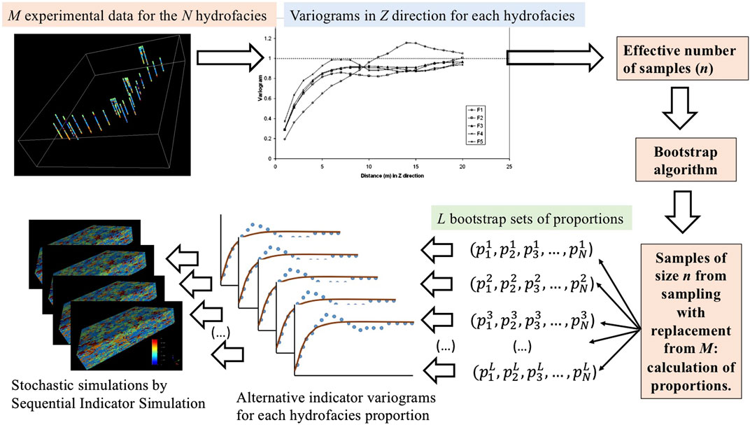
FIGURE 1. Flowchart for the proposed methodology.

A fundamental issue is the determination of the effective number of samples from the correlated experimental data. We use aligned, contiguous sequences of data, such as strings of borehole cores, to determine the effective number of data to be used for resampling. The effective range of the variogram in the vertical direction is a key parameter because the variability along the boreholes is much greater than the horizontal variability between boreholes. An example of this determination is given in the case study section.

Once the effective number of data is determined, a large number of samples (several thousand) of that size is obtained by sampling with replacement from the full data set. For each sample the hydrofacies proportions are calculated and a histogram is generated for each hydrofacies. Note that, as the proportions of hydrofacies must be used jointly (for example, to satisfy Eq. 14), it is the proportions of the resamples that are retained, and each vector of proportions is used in the geostatistical simulation rather than using the estimated proportions from the data.

The sequential simulation algorithm uses the models fitted to the experimental variograms. Emery (2004) provides a critical appraisal of the limitations of sequential indicator simulation in general; those that relate to categorical variables are addressed in the approach described in this paper. There are several possibilities for estimating the probabilities in Eq. 14. These range from simple indicator kriging, in which each indicator variable has an anisotropic variogram specific to each indicator variable, to full indicator cokriging. Although the latter is the best and most complete approach, there are serious issues around model inference and some simplification is required. For example, a common model could be used for all cross-variograms with a scaling factor applied to each of them so that the correct sill, as given in Eq. 12, is assigned. However, this approach is constrained by the need to satisfy the model validity requirement for a positive definite coregionalization model. For categorical variables a valid model has a very clear physical meaning. Once an arbitrary facies, $F_i=\left\{\mathrm{u}|f\left(\mathrm{u}\right)=i\right\}$ is fixed at an arbitrary location u then the same hydrofacies, $F_i$, occurs at any other arbitrary location $\mathrm{u}+\mathrm{h}$ with conditional probability $\frac{C_{ij}\left(\mathrm{h}\right)}{p_j}=\frac{\left(p_i- {\gamma }_i\left(\mathrm{h}\right)\right)}{p_i}$ and hydrofacies $F_j$ (for $j\ne i$) occurs with conditional probability $\frac{C_{ij}\left(\mathrm{h}\right)}{p_j}= -\frac{{\gamma }_{ij}\left(\mathrm{h}\right)}{p_j}$. In addition, writing $C_i\left(\mathrm{h}\right)= C_{ii}\left(\mathrm{h}\right)$, the total probability must be:

${\displaystyle \sum }_{j=1}^N\frac{C_{ij}\left(\mathrm{h}\right)}{p_j} = 1(15)$

Equation (15), written in terms of the non-centred covariance, can also be written in terms of variograms or in terms of centered covariances, $\sigma \left(\mathrm{h}\right)$:

${\displaystyle \sum }_{j=1}^N\frac{{\sigma }_{ij}\left(\mathrm{h}\right)+ p_i{p}_j}{p_j} = 1(16)$

$-{\displaystyle \sum }_{j=1}^N{\gamma }_{ij}\left(\mathrm{h}\right) = 0(17)$

Note that, by writing ${\gamma }_i\left(\mathrm{h}\right)= {\gamma }_{ii}\left(\mathrm{h}\right)$, Eqs 17 and 10 are equivalent. That is, a valid model of covariance and cross-covariances implies the occurrence probabilities are coherent.

From a practical perspective, there is also a need to demonstrate that any improvement in results from the complete cokriging method is sufficient to justify its use over that of simpler approaches. Thus, simple indicator kriging, in which each indicator variable has a specific anisotropic variogram, was chosen for the work presented in this paper.

The technique is illustrated in detail by the case study in the following section.

Case Study

The study area (Figure 2A) is the detrital aquifer of the Andarax river delta in the province of Almeria in southern Spain. The aquifer comprises deltaic deposits from the Pleistocene overlain by fluvial and deltaic deposits from the Quaternary (Sánchez-Martos et al., 1999). The Andarax river is ephemeral, with flow usually resulting from big storms, and is an example of rivers in the semi-arid coastal regions of the Mediterranean. Within the study area there are 19 boreholes and three clusters of four piezometers each (Jorreto-Zaguirre et al., 2005) the locations of which are shown in plan view in Figure 2A. Figure 2B shows the spatial locations of the boreholes and piezometers together with colour-coded plots of the recorded hydrofacies. The vertical resolution of the boreholes and piezomenter cores is one m. The borehole cores have been classified into five types of hydrofacies according to their permeability: very permeable (F1), permeable (F2), low permeability (F3), impermeable (F4), and very impermeable (F5).

FIGURE 2

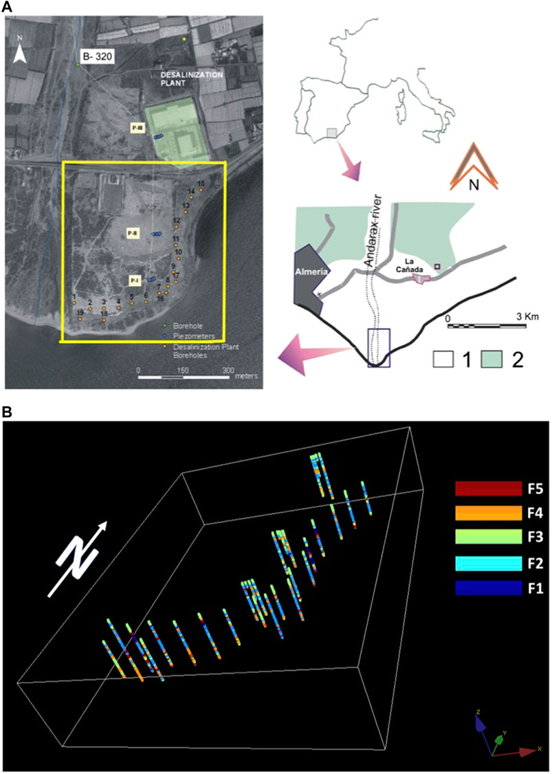
FIGURE 2. (A) Location of the study area in the Andaraxriver delta. The yellow square is the area of the case study in which there are 19 boreholes and three clusters of four piezometers. The numeral 1 denotes detrital material from the Quaternary and 2 from the Pliocene. (B) Data for the five hydrofacies (F1 to F5) within boreholes and piezometers. The color legend ranges from very permeable (dark blue = F1) to very impermeable (dark red = F5).

The proportions of each hydrofacies measured along the boreholes are: 2.62, 43.72, 27.21, 18.57, and 7.87%, respectively. The problem could be simplified by grouping the hydrofacies into three broader types (aquifer, aquitard and aquiclude) or even into only two types (permeable and impermeable). However, there is value in retaining the five hydrofacies because the very permeable hydrofacies could be associated with high permeability channels while the very impermeable facies could be associated with hydraulic barriers. Figure 2B clearly shows the sparsity of the data, with very few borehole cores to represent the total study volume, from which it is reasonable to conclude that the real hydrofacies proportions may differ significantly from the estimated values.

The data comprise hydrofacies observations made on 2,477 one-metre borehole cores. Classical (non-spatial) statistics cannot be used to evaluate the uncertainty of the proportions calculated from these data because spatial correlation implies that neighboring samples are not independent and, therefore, some of the information in the values of these samples is redundant. Variograms can be used to quantify the range of spatial correlation from which it is possible to infer the effective number of (spatially uncorrelated) samples. Variograms calculated along the boreholes (Figure 3) indicate an effective range of spatial correlation in this direction of around 8 m, i.e., samples separated by distances greater than, or equal to, 8 m are uncorrelated. Assuming that the average distance between pairs of boreholes is greater than the ranges of spatial correlation in all other directions, the effective number of data can be inferred as approximately 300. The uncertainty of the proportions can now be estimated by a bootstrap procedure, that is, resampling with replacement with a sample size of 300 from the full set of 2,477 data. A total of 5,000 bootstrap samples of size 300 were generated and the bootstrap distribution of the proportion of each of the five categories was calculated. Figure 4A shows the bootstrap distribution for the very permeable (F1) hydrofacies. Confidence intervals can be calculated from the bootstrap distributions. For example, although the estimated proportion of the very permeable hydrofacies (F1) is 2.62%, the lower and upper limits of the 95% confidence interval are, respectively, 1% and 4%. Figure 4B shows the bootstrap distribution for the very impermeable hydrofacies (F5). The complete results are shown in Table 1 from which the similarity between mean and median indicates that the distributions are symmetrical.

FIGURE 3

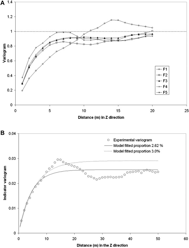
FIGURE 3. (A) Standardized indicator variograms calculated along the boreholes for the five hydrofacies and standardized by their variances. (B) Indicator variogram of facies F1 along the borehole and the two best models fitted which were those for hydro facies F1 proportions of 2.62 and 3.00% which implies variances of 0.0255 and 0.0291, respectively, and fitted ranges of 4.37 and 5.62 m, respectively, for an exponential variogram model.

FIGURE 4

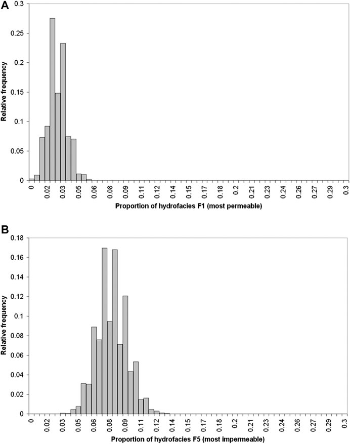
FIGURE 4. Histogram of the bootstrap distribution for (A) F1 hydrofacies and (B) F5 hydrofacies.

TABLE 1

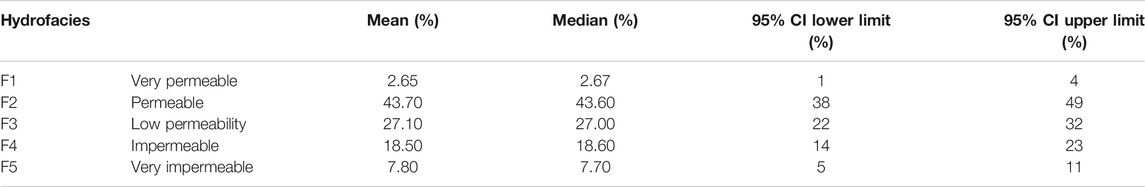
TABLE 1. Statistics of the bootstrap distributions for the different hydrofacies.

Variograms were calculated for each of the indicators. As the sills of the direct and cross-variograms depend on the hydrofacies proportions it is useful to standardize the experimental variograms using the estimated proportions so that they can be displayed on the same graph. Figure 3A shows the standardized variograms calculated along the boreholes. The variogram for hydrofacies F1 is noticeably different to those of the other hydrofacies; the variogram for F5 also differs from the others but by a smaller amount. None of the variograms in Figure 3A reach the theoretical sill of 1.0, which reflects the fact that the estimated proportions differ from the true underlying proportions. The implication of this observation is that models fitted to the sample variograms will be different for each bootstrap sample of proportions. Table 2 lists the experimental proportions together with the proportions calculated from the first ten bootstrap samples and Figure 3B shows the experimental variograms for hydrofacies F1. An indication of the effects of the uncertainty of the proportions is given by comparing the variograms of the experimental proportion of hydrofacies F1 (2.62%) with, for example, the fifth bootstrap value of 3.00%. These two proportions would generate respective variogram sills of 0.0255 and 0.0291 and weighted least squares estimated ranges of 4.37 and 5.62 m, respectively, as shown in Figure 4B. The weighted least squares estimated ranges of exponential models for the experimental proportions of the other hydrofacies are 3.00, 2.87, 2.73, and 2.05 m for F2, F3, F4, and F5, respectively, and these values quantify the differences that can be seen graphically in Figure 3A. Note that for exponential model variograms the sill is reached asymptotically and it is useful to define an effective, or practical, range at which, for all practical purposes, the sill is reached; the effective range is three times the range parameter in the variogram model.

TABLE 2

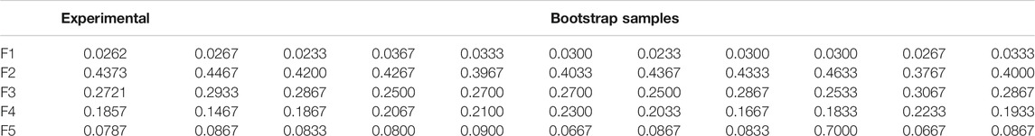
TABLE 2. Experimental proportions and first ten bootstrap realisations of proportions.

Although the locations of the boreholes are not ideal for detecting horizontal anisotropies, there is no evidence of anisotropy in the horizontal plane as demonstrated by the example of the east-west and north-south indicator variograms for hydrofacies F5 in Figure 5. However, because of the physical structure of deltaic deposits, anisotropies are expected between vertical and horizontal directions and these should be evident in the variograms, i.e., spatial correlation in the horizontal plane should be greater than that in the vertical direction. Given the lack of evidence for anisotropy in the horizontal plane, omni-directional horizontal variograms were calculated and modeled. The exponential models fitted by weighted least squares to the omni-directional variograms in the horizontal plane for the different hydrofacies have ranges of 6.8, 27.5, 35.8, 25.5, and 25.4 m for hydrofacies F1 to F5, respectively. The very high permeability hydrofacies (F1) has an effective range, or spatial correlation length, of 21 m and the rest of the hydrofacies have effective ranges of 75–105 m.

FIGURE 5

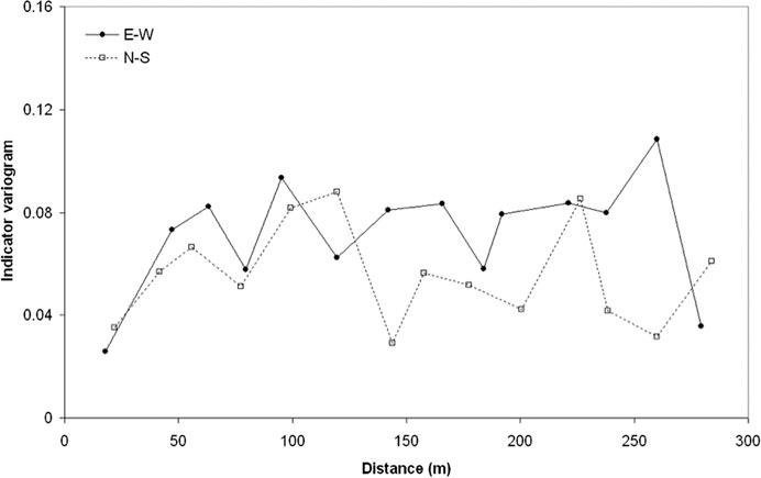
FIGURE 5. Indicator variograms for hydrofacies F5 for the two perpendicular directions most likely to exhibit anisotropic behavior.

A plausible explanation of these variograms is that the effective ranges quantify the average horizontal extents of permeability channels. If, for example, permeability is due to paleochannels formed from meandering streams then the greater the horizontal extent of the hydrofacies the greater is the likelihood for hydraulic barriers to have formed. Thus, the highest permeability facies F1 has the smallest horizontal extent (21 m) and the lower permeability facies have horizontal extents greater than 75 m.

For the co-regionalization model of the five hydrofacies, Figure 6 shows the experimental indicator cross-variograms along the boreholes between hydrofacies F2 and the other four hydrofacies and the models fitted to them. Figure 7 shows the experimental indicator variogram along the boreholes of hydrofacies F2 and the model fitted to it. The models were fitted by taking account of the experimental proportions and using weighted least squares to fit an exponential model with no nugget. The model fitted to the indicator cross-variogram between hydrofacies F2 and F1 has a range of 7.45 m while the indicator direct-variograms of those hydrofacies have ranges of 3.0 and 4.37 m, respectively. However, these ranges are not compatible with the linear model of coregionalization in which the range of the cross-variogram cannot be greater than the ranges of the direct variograms. The consequence of failing to meet this requirement can be demonstrated in terms of the conditional probabilities of occurrence. If, for example, hydrofacies F2 is observed at an arbitrary location u, what is the probability that each of the hydrofacies occurs at, say, 5 m further down the borehole?

FIGURE 6

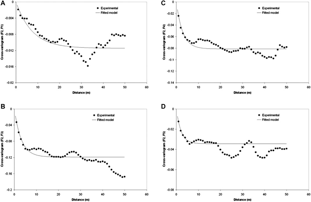
FIGURE 6. Indicator cross-variograms between hydrofacies F2 and the other hydrofacies and models fitted to them: (A) F2-F1; (B) F2-F3; (C) F2-F4 and (D) F2-F5.

FIGURE 7

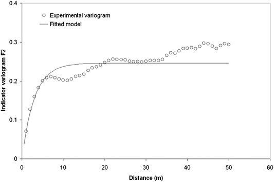
FIGURE 7. Indicator variograms for hydrofacies F2 and fitted model.

These probabilities can be calculated from the models fitted to the direct and cross variograms as follows:

Probability of F2 occurring:

$\frac{C_2\left(5\right)}{p_2}=\frac{\left(p_2- {\gamma }_2\left(5\right)\right)}{p_2}=\frac{\left(0.4372- {\gamma }_2\left(5\right)\right)}{0.4372} = 0.543$

Probability of F1 occurring:

$\frac{C_{21}\left(5\right)}{p_{21}} =\frac{{\gamma }_{21}\left(5\right)}{p_1}= 0.213$

Probability of F3 occurring:

$\frac{C_{21}\left(5\right)}{p_{23}}=\frac{-{\gamma }_{23}\left(5\right)}{p_3}=0.347$

Probability of F4 occurring:

$\frac{C_{24}\left(5\right)}{p_{24}}=\frac{-{\gamma }_{24}\left(5\right)}{p_4}=0.361$

Probability of F5 occurring:

$\frac{C_{25}\left(5\right)}{p_{25}}=\frac{-{\gamma }_{25}\left(5\right)}{p_5}=0.394$

The sum of these probabilities is 1.86 rather than 1.0 as it should be and thus the models fitted in Figures 6, 7 are not valid when taken jointly. The ranges could be modified to ensure that the total probability is 1.0 by increasing the ranges of the indicator cross-variograms. However, this is not a general solution because the example given is very specific: it is only for one hydrofacies, for the Z-direction variogram, using only one conditioning point and for a specific distance of 5 m. Fitting models that would satisfy all possible constraints would be very cumbersome.

If only the direct variograms are used, the probability of F2 occurring remains the same:

$\frac{C_2\left(5\right)}{p_2} = \frac{\left(p_2- {\gamma }_2\left(5\right)\right)}{p_2} = \frac{\left(0.4372- {\gamma }_2\left(5\right)\right)}{0.4372} = 0.543$

and the complementary probability 1–0.543 = 0.457 is distributed among F1, F3, F4, and F5 in proportion to their prior probabilities of 0.0262, 0.2721, 0.1857, and 0.0787, respectively. Using these values in the previous equation would reproduce the correct variograms.

The following procedure was adopted for sequential simulation:

(a) Retain each bootstrap realization of the hydrofacies proportions that is inside the 95% confidence interval $\left\{{\widehat{p}}_i>0, i=1, . . . ,5\right\}$ . This automatically satisfies the requirement: ${\displaystyle \sum }_{i=1}^5{\widehat{p}}_i=1.$

(b) Using ${\widehat{p}}_i\left(1-{\widehat{p}}_i\right)$ for the sill of each direct variogram and $-{\widehat{p}}_i{\widehat{p}}_j$ for the sill of each cross-variogram, determine, by least squares, the ranges that give the best fit of exponential model variograms to the experimental variograms.

(c) Apply the sequential simulation algorithm.

(d) Go to (a) and repeat to generate a specified number of simulations.

For the experimental proportions, the least squares fit to the direct and cross-variograms of an exponential model without a nugget gives the ranges shown in Table 3. The effective ranges, or distances beyond which correlations are effectively zero, are three times these values.

TABLE 3

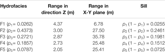
TABLE 3. Ranges of an exponential variogram model fitted to the experimental variogram by weighted least squares taking into account the experimental proportions.

There are three general possibilities for modeling the conditional probabilities of categorical variables (Goovaerts, 1994) for the purpose of simulating them by sequential indicator simulation: median indicator kriging, multiple indicator kriging and indicator co-kriging. Median indicator kriging uses the same indicator variogram model for all categories; this common model is a type of mean, or median, model. The second possibility is multiple indicator kriging using variogram models fitted to each hydrofacies indicator.

The third possibility is indicator co-kriging in which the main difficulty is to fit a valid coregionalization model. The simplest coregionalization model is the linear model in which all direct, and cross, variograms are linear combinations of a set of basic direct variograms. The intrinsic coregionalization model is a special case of the linear model in which the basic direct variograms for each variable are identical. Allowing for the noisy nature of the empirical variograms and cross-variograms in Figures 8A,B for the horizontal plane (shown as dots in the figure), it is reasonable to fit the same model for all directions as shown by the red lines. A different model is fitted for the variograms in the vertical direction, but the model is the same for the direct and cross-variograms. As this model is an intrinsic model of coregionalization and, because all variables (the five indicators of the five hydrofacies) have been measured at all locations, it has the property of auto-krigeability (Wackernagel, 1994), which means that cokriging a variable from the set of coregionalized variables yields the same value as kriging.

FIGURE 8

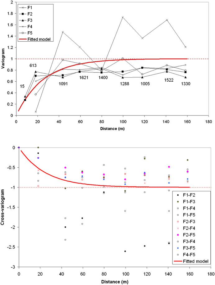
FIGURE 8. (A) Standardized indicator direct variogram for the five hydrofacies and fitted model. (B) Standardized indicator cross-variograms for the five hydrofacies: ten cross-variograms and fitted model. The fitted model is an intrinsic model of coregionalization. The model is exponential with range 25 m (effective range of 75 m).

The intrinsic correlation model can be written as:

$\text{ Γ}\left(h\right)=\mathrm{C} \gamma \left(h\right)(18)$

where γ (h) is an exponential model variogram with range 25 m as shown in Figure 8, and C is a positive definite matrix of coefficients:

$\mathrm{C} = \left[\begin{array}{ccccc}{p}_1\left(1-p_1\right)& -p_1{p}_2& -p_1{p}_3& -p_1{p}_4& -p_1{p}_5\\ -p_2{p}_1& p_2\left(1-p_2\right)& -p_2{p}_3& -p_2{p}_4& -p_2{p}_5\\ -p_3{p}_1& -p_3{p}_2& p_3\left(1-p_3\right)& -p_3{p}_4& -p_3{p}_5\\ -p_4{p}_1& -p_4{p}_2& -p_4{p}_3& p_4\left(1-p_4\right)& -p_4{p}_5\\ -p_5{p}_1& -p_5{p}_2& -p_5{p}_3& -p_5{p}_4& p_5\left(1-p_5\right)\end{array}\right](19)$

Furthermore, from Eq. 10 these coefficients must be such that:

$\begin{array}{c}{\gamma }_1\left(h\right)= -{\gamma }_{12}\left(h\right)- {\gamma }_{13}\left(h\right)- {\gamma }_{14}\left(h\right)- {\gamma }_{15}\left(h\right)\\ {\gamma }_2\left(h\right)= -{\gamma }_{21}\left(h\right)- {\gamma }_{23}\left(h\right)- {\gamma }_{24}\left(h\right)- {\gamma }_{25}\left(h\right)\\ {\gamma }_3\left(h\right)= -{\gamma }_{31}\left(h\right)- {\gamma }_{32}\left(h\right)- {\gamma }_{34}\left(h\right)- {\gamma }_{35}\left(h\right)\\ {\gamma }_4\left(h\right)= -{\gamma }_{41}\left(h\right)- {\gamma }_{42}\left(h\right)- {\gamma }_{43}\left(h\right)- {\gamma }_{45}\left(h\right)\\ {\gamma }_5\left(h\right)= -{\gamma }_{51}\left(h\right)- {\gamma }_{52}\left(h\right)- {\gamma }_{53}\left(h\right)- {\gamma }_{54}\left(h\right)\end{array}(20)$

Using median indicator kriging gives unrealistic outputs, in particular hydrofacies models with connectivities that are too low to generate observed flows. In this work, multiple indicator kriging was used together with the auto-krigeability model in which the cross-variogram of each variable with all other variables is proportional to the variogram of that variable.

This approach allows for different spatial variability for each hydrofacies and it generates realisations with significantly higher connectivity than those generated by median indicator kriging as can be seen by comparing Figures 9A,B. Figure 10 shows three-dimensional views of four simulations using the experimental proportions; these views provide a better appreciation of the relationships between the different hydrofacies and of the real heterogeneity of the aquifer. This heterogeneity may influence the spatial patterns of seawater intrusion and thus condition the spatial distribution of water quality.

FIGURE 9

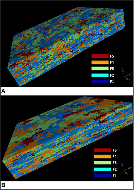
FIGURE 9. 3D view of a realization generated by using the experimental proportions and (A) median indicator kriging and (B) multiple indicator kriging.

FIGURE 10

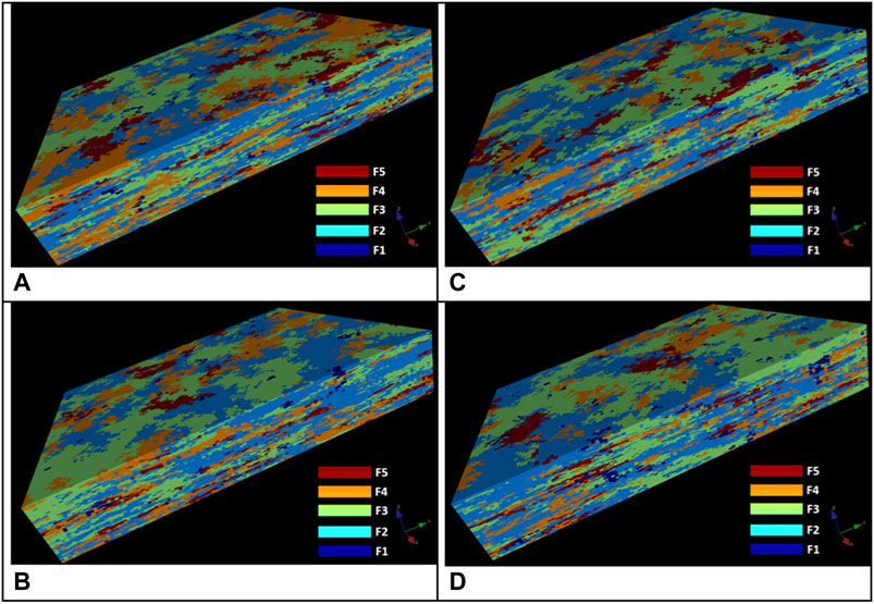
FIGURE 10. 3D views of four simulations using the experimental proportions (A) simulation 1; (B) simulation 2; (C) simulation 3; (D) simulation 4.

Some examples of the direct- and cross-variograms reproduced by the method are shown in Figures 11, 12 for the Z-direction and the horizontal plane, respectively. The ergodic fluctuations of the variograms of the simulation may not seem large enough to include the experimental variogram, but it should be remembered that only the experimental proportions were used and not the bootstrap proportions. When the bootstrap proportions are used, the sills of the variogram models used in the simulation change, as do the ranges, and this increases the ergodic fluctuation to reflect the unknown real variability of the hydrofacies. This would be apparent in an application in which thousands of simulations are used in order to include the spatial uncertainty of the hydrofacies in the simulation.

FIGURE 11

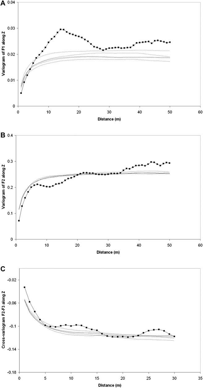
FIGURE 11. Variograms of the borehole data (solid line) and the simulations (dashed lines) calculated for the vertical direction. (A) Variogram of hydrofacies F1. (B) Variogram of hydrofacies F2 and (C) Cross-variogram of hydrofacies F2 and F3.

FIGURE 12

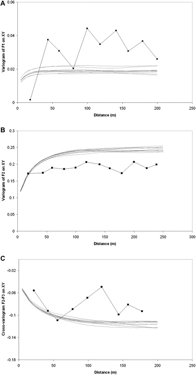
FIGURE 12. Variogram of the borehole (solid line) data and from the simulations (dashed lane) calculated along the horizontal direction. (A) Variogram of hydrofacies F1. (B) Variogram of hydrofacies F2 and (C) cross-variogram of hydrofacies F2 and F3.

Finally, Figures 13A,B show the connectivity function (Pardo-Igúzquiza and Dowd, 2003) for the five hydrofacies in the vertical direction and on the horizontal plane, respectively. For hydrofacies facies F1, for example, there are connectivities of up to 40 m in the vertical direction and 100 m in the horizontal direction, which, because these are very high permeability channels, may have important consequences for water intrusion and/or for rapid propagation of contaminants.

FIGURE 13

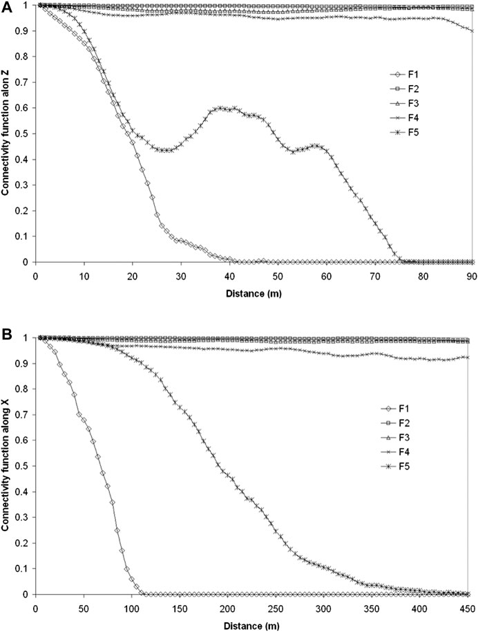
FIGURE 13. Connectivity function for the different hydrofacies. (A) Vertical direction. (B)X direction.

Discussion

The conditional geostatistical simulation of hydrofacies provides numerical models of aquifers that reproduce the observed spatial variability of the geological structures. These patterns of spatial variability significantly influence flow and transport modeling in coastal aquifers and, as a consequence, influence the assessment of seawater intrusion. This is because the spatial variability of the hydrofacies influences the mechanical macro-dispersion of the mixed zone in seawater intrusion.

This work shows that the uncertainty in hydrofacies proportions estimated from sparse data can be included in sequential simulation. These proportions condition the sills of the variogram models, the variability of which provides a measure of the impact of the uncertainty in fitting theoretical models.

Various approaches have been used to simulate categorical variables using indicators. Each of these uses different types of indicator kriging in the sequential simulation algorithm. The work presented in this paper uses indicator kriging, in which each hydrofacies has its own model, as a compromise between simpler options and the most complete option of full cokriging. The connectivity function given in Pardo-Igúzquiza and Dowd (2003) has been used as a measure of connectivity although other connectivity indices could have been used, for example, Vassena et al. (2010) and Renard and Allard (2013).

Although the work presented here is limited to the simulation of categorical variables, it can easily be extended to include the generation of quantitative variables (e.g., hydraulic conductivity, porosity) by assigning a probability density function of the variable to each categorical hydrofacies. Borehole logging (natural gamma and resistivity are available) could be used to construct the probability functions. Another extension would be to use pumping test data for screening the simulated realisations. All these lines of research are left open for future work.

A fundamental question that arises from this study is whether the inclusion of the uncertainty of the hydrofacies proportions in the simulation (a large number of realisations considering the bootstrap proportions) gives results that are significantly different to those that would be obtained from a standard simulation (i.e. a large number of realisations with the same global proportion, but ignoring the uncertainty of the hydrofacies proportions). To answer this question, we used a simplified experiment to compare the outputs from the proposed extended sequential indicator simulation with those that would be obtained from standard sequential indicator simulation. The experiment comprised:

• A two-dimensional problem.

• Only two facies: the most permeable phase (0) and all others (1).

• Non-conditional simulations.

• 1,000 independent simulations.

• Identical variograms for the proposed extended sequential indicator simulation and the standard sequential indicator simulation.

• The same experimental proportions were used for all of the 1,000 standard sequential indicator simulations.

• 1,000 bootstrapped proportions were used for the 1,000 simulations using the proposed extended sequential indicator simulations.

An assessment of the connectivity of the two approaches showed that the means of the connectivity function statistics and the means of the connectivity function itself are very similar. However, the minimum and maximum numbers of connected components in a single simulation are significantly different with a greater range of variation in the simulations generated by the proposed extension. The minimum and maximum number of connected components for a standard sequential indicator simulation were 19 and 65, respectively whereas for the extended sequential indicator simulation they were 4 and 95, respectively. Thus, the variability is significatively larger when the uncertainty of the facies proportions is included. In addition, the same constant variograms (type of variogram and range) were used in both sets of 1,000 realisations. However, the ranges of the variograms will change in the proposed approach because the proportions are related to the sill and thus the ranges fitted to the experimental variograms may be different. This would further increase the variability of the extended sequential indicator simulations.

In this test, the propagation of uncertainty from the facies proportions into the set of simulations is significant and we conclude that the same must be so in the three-dimensional case with significantly more hydrofacies than were used in this demonstration.

Conclusions

An extension of sequential indicator simulation for simulating realisations of the three-dimensional distribution of deltaic hydrofacies has been proposed in this paper. The extension is the inclusion of the uncertainty of the proportions of each hydrofacies by using a bootstrap algorithm that generates feasible realisations of the proportions using an effective number of samples to evaluate that uncertainty. The actual proportions of the hydrofacies influence the direct and cross-variograms of the hydrofacies (using indicators) and thus affect the connectivity between them. This extension will allow a more realistic evaluation of the uncertainty of the underground geological medium which, in turn, will affect the simulation of flow and transport in coastal aquifers.

Data Availability Statement

All datasets presented in this study are included in the article/Supplementary Material.

Author Contributions

SJ collected the data and studied the hydrofacies as part of her PhD. She participated in the design and structure of the paper. PD participated in the geostatistical analysis of the data and the writing of the paper. EP conducted the geostatistical simulations and participated in the writing of the paper. AP participated in the design of the data collection, their interpretation and the drawing of the figures. FS participated in the geological interpretation of the study area and the data as well as in the interpretation of the results.

Conflict of Interest

The authors declare that the research was conducted in the absence of any commercial or financial relationships that could be construed as a potential conflict of interest.

Funding

This work was supported by Research Projects CGL 2010–15498 and CGL 2007–63450 del Ministerio de Economía y Competitividad, Spain and by the Australian Research Council Discovery Grant DP110104766.

Acknowledgments

We thank the four reviewers for their constructive criticism that has helped significantly to improve the final version of this paper.

Supplementary Material

The Supplementary Material for this article can be found online at: https://www.frontiersin.org/articles/10.3389/feart.2020.563122/full#supplementary-material

References

Barakat, M. K. A. (2010). Modern geophysical techniques for constructing a 3D geological model on the Nile Delta, Egypt. MS Dissertation. Berlin (Germany): Technische Universität Berlin, 158.

Google Scholar

Bianchi, M., Zheng, C., Wilson, C., Tick, G. R., Liu, G., and Gorelick, S. M. (2011). Spatial connectivity in a highly heterogeneous aquifer: from cores to preferential flow paths. Water Resour. Res. 47, W05524. doi:10.1029/2009wr008966

CrossRef Full Text | Google Scholar

Cabello, P., Cuevas, J. L., and Ramos, E. (2007). 3D modelling of grain size distribution in quaternary deltaic deposits (Llobregat Delta, NE Spain). Geol. Acta. 5, 231–244. doi:10.1344/105.000000296

Google Scholar

Carle, S. F., and Fogg, G. E. (1996). Transition probability-based indicator geostatistics. Math. Geol. 28, 453–476. doi:10.1007/bf02083656

CrossRef Full Text | Google Scholar

Chilès, J.-P., and Delfiner, A. (1999). Geostatistics: modelling spatial uncertainty. New York, NY: Wiley-Interscience, 695.

Google Scholar

Comunian, A., Renard, P., Straubhaar, J., and Bayer, P. (2011). Three-dimensional high resolution fluvio-glacial aquifer analog - Part 2: geostatistical modeling. J. Hydrol. 405, 10–23. doi:10.1016/j.jhydrol.2011.03.037

CrossRef Full Text | Google Scholar

Deidda, G. P., Ranieri, G., Uras, G., Consentino, P., and Martorana, R. (2006). Geophysical investigations in the flumendosa river delta, Sardinia (Italy) — seismic reflection imaging. Geophysics 71, 1JA–Z75. doi:10.1190/1.2213247

CrossRef Full Text | Google Scholar

dell’Arciprete, D., Bersezio, R., Felleti, F., Giudici, M., Comunian, A., and Renard, P. (2012). Comparison of three geostatistical methods for hydrofacies simulation: a test on alluvial sediments. Hydrogeol. J. 20, 299–311. doi:10.1007/s10040-011-0808-0

CrossRef Full Text | Google Scholar

Deutsch, C. V., and Journel, A. G. (1998). GSLIB: geostatistical software library and user´s guide. 2nd Edn. New York, NY: Oxford University Press, 340.

CrossRef Full Text | Google Scholar

Dowd, P. A., Pardo-Igúzquiza, E., and Xu, C. (2003). Plurigau: a computer program for simulating spatial facies using the truncated plurigaussian method. Comput. Geosci. 29, 123–141. doi:10.1016/s0098-3004(02)00070-5

CrossRef Full Text | Google Scholar

Dubrule, O., and Damsleth, E. (2001). Achievements and challenges in petroleum geostatistics. Petrol. Geosci. 7, S1–S7. doi:10.1144/petgeo.7.s.s1

CrossRef Full Text | Google Scholar

Eaton, T. T. (2006). On the importance of geological heterogeneity for flow simulation. Sediment. Geol. 184, 187–201. doi:10.1016/j.sedgeo.2005.11.002

CrossRef Full Text | Google Scholar

Emery, X. (2004). Properties and limitations of sequential indicator simulation. Stoch. Environ. Res. Risk Assess. 18, 414–424. doi:10.1007/s00477-004-0213-5

CrossRef Full Text | Google Scholar

Falivene, O., Cabrera, L., Muñoz, J. A., Arbués, P., Frenández, O., and Sáez, A. (2007). Statistical grid-based facies reconstruction and modelling for sedimentary bodies. Alluvial-palustrine and turbiditic examples. Geol. Acta. 5, 199–230. doi:10.1344/105.000000295

CrossRef Full Text | Google Scholar

Goovaerts, P. (1994). “Comparison of COIK, IK and MIK performances for modelling conditional probabilities of categorical variables,” in Geostatistics for the next century. Editor R. Dimitrakopoulos, The Netherlands: Kluwer Academic Publishers, 18–29.

Google Scholar

Goovaerts, P. (1997). Geostatistics for natural resources evaluation. Oxford, UK: Oxford University Press, 502.

Google Scholar

Gouw, M. J. P. (2007). Alluvial architecture of fluvio-deltaic successions: a review with special reference to Holocene settings. The Netherlands J. Geosci. 86, 211–227. doi:10.1017/s0016774600077817

CrossRef Full Text | Google Scholar

Jorreto-Zaguirre, S., Pulido-Bosch, A., Gisbert-Gallego, J., and Sánchez-Martos, F. (2005). Las diagrafías y la caracterización de la influencia de los bombeos de agua de mar sobre el acuífero del delta del Andarax (Almería). Ind. Miner. 362, 15–21.

CrossRef Full Text | Google Scholar

Journel, A., and Alabert, F. (1989). Non-gaussian data expansion in the earth sciences. Terra. Nova. 1, 123–134, doi:10.1111/j.1365-3121.1989.tb00344.x.

CrossRef Full Text | Google Scholar

Lee, S.-Y., Carle, S. F., and Fogg, G. E. (2007). Geologic heterogeneity and a comparison of two geostatistical models: sequential Gaussian and transition probability-based geostatistical simulation. Adv. Water Resour. 30, 1914–1932. doi:10.1016/j.advwatres.2007.03.005

CrossRef Full Text | Google Scholar

Le Loc’h, G., Beucher, H., Galli, A., and Doligez, B. (1994). Improvement in the truncated gaussian method: combining several gaussian functions. Conference proceedings ECMOR IV, Fourth european conference on the mathematics of oil recovery, Røros, Norway, June, 7–10 1994 (European Association of Geoscientists & Engineers).

Google Scholar

Le Loc’h, G., and Galli, A. (1996). “Truncated Pluri-Gaussian method: theoretical and practical points of view,” in Geostatistics Wollongong’96. Editors Baafi, et al. , (Dordrecht, Netherlands: Kluwer), Vol. 1, 211–222.

Google Scholar

Mariethoz, G., Renard, P., Cornaton, F., and Jaquet, O. (2009). Truncated plurigaussian simulations to characterize aquifer heterogeneity. Ground Water. 47, 13–24. doi:10.1111/j.1745-6584.2008.00489.x

CrossRef Full Text | Pubmed | Google Scholar

Myers, D. E. (1989). To be or not to be… stationary? That is the question…Stationary? That is the question. Math. Geol. 21, 347–362. doi:10.1007/bf00893695

CrossRef Full Text | Google Scholar

Pardo-Igúzquiza, E., and Dowd, P. A. (2003). CONNEC3D: a computer program for connectivity analysis of 3D random set models. Comput. Geosci. 29, 775–785. doi:10.1016/s0098-3004(03)00028-1

CrossRef Full Text | Google Scholar

Pardo-Iguzquiza, E., Chica-Olmo, M., Luque-Espinar, J. A., and Garcia-Soldado, M. J. (2009). Using semi-variogram parameter uncertainty in hydrogeological applications. Groundwater 41 (1), 25–34. doi:10.1111/j.1745-6584.2008.00494.x

CrossRef Full Text | Google Scholar

Perulero, R., Guadagnini, L., Riva, M., Giudici, M., and Guadagnini, A. (2014). Impact of two geostatistical hydro-facies simulation strategies on head statistics under non-uniform groundwater flow. J. Hydrol. 508, 343–355. doi:10.1016/j.jhydrol.2013.11.009

CrossRef Full Text | Google Scholar

Renard, P., and Allard, D. (2013). Connectivity metrics for subsurface flow and transport. Adv. Water Resour. 51, 168–196. doi:10.1016/j.advwatres.2011.12.001

CrossRef Full Text | Google Scholar

Sanchez Martos, F., Bosch, A. P., and Calaforra, J. M. (1999). Hydrogeochemical processes in an arid region of Europe (Almeria, SE Spain). Appl. Geochem. 14, 735–745. doi:10.1016/s0883-2927(98)00094-8

CrossRef Full Text | Google Scholar

Strebelle, S. (2002). Conditional simulation of complex geological structures using multiple-point statistics. Math. Geol. 34, 1–21. doi:10.1023/a:1014009426274

CrossRef Full Text | Google Scholar

Tercier, P., Knight, R., and Jol, H. (2000). A comparison of the correlation structure in GPR images of deltaic and barrier‐spit depositional environments. Geophysics 64, 1028–1340. doi:10.1190/1.1444807

CrossRef Full Text | Google Scholar

Vassena, C., Cattaneo, L., and Giudici, M., (2010). Assessment of the role of facies heterogeneity at the fine scale by numerical transport experiments and connectivity indicators. Hydrogeol. J. 18, 651–668. doi:10.1007/s10040-009-0523-2

CrossRef Full Text | Google Scholar

Wackernagel, H. (1994). Cokriging versus kriging in regionalized multivariate data analysis. Geoderma 62, 83–92. doi:10.1016/0016-7061(94)90029-9

CrossRef Full Text | Google Scholar