Quantifying Downstream, Vertical and Lateral Variation in Fluvial Deposits: Implications From the Huesca Distributive Fluvial System

Introduction

A global remote-sensing study on over 700 modern continental sedimentary basins has shown that fluvial sedimentation patterns are dominated by distributive fluvial systems (DFS) (Hartley et al., 2010a). DFS are observed to be prevalent in all climatic and tectonic settings within sedimentary basins, and as sedimentary basins are areas in which accommodation and active sedimentation occurs, it is hypothesized that DFS should be an important component of the fluvial geologic record (Hartley et al., 2010a; Weissmann et al., 2010, 2015). Weissmann et al. (2015) provide further analyses on modern sedimentary basins, quantifying the aerial distribution of fluvial geomorphic features in a variety of selected sedimentary basins. Their analyses showed that in the basins studied, DFS constituted 88% of fluvial deposits with tributary (confined) systems accounting for <12%. Although not without controversy (e.g., Hartley et al., 2010b; Sambrook-Smith et al., 2010; Fielding et al., 2012), and debate ensues as to whether alluvial fans should be treated differently to DFS (see Ventra and Clarke, 2018 for discussion), the terminology and concept has been widely adopted (Ventra and Clarke, 2018).

Weissmann et al. (2011) note that whilst analysis of modern satellite imagery is a powerful tool for understanding modern day DFS, it only provides a ‘snapshot’ in time. To fully understand the processes that operate on DFS and how they develop through time the study of ancient deposits is needed. DFS can contain a wealth of resources in the form of oil and gas (e.g., Moscariello, 2005; Kukulski et al., 2013); mineral deposits (Peterson, 1977; Turner-Peterson, 1986; Owen et al., 2016) and be aquifers (Weissmann et al., 1999; 2002; 2004; van Dijk et al., 2016). Currently, outcrop analogues are used to aid subsurface exploration to better understand the distribution and connectivity of reservoir bodies, as well as aid paleogeographic reconstructions. Although qualitative descriptions are present for DFS (e.g., Nichols, 1987; Kelly and Olsen, 1993; Willis, 1993a; Willis, 1993b; Nichols and Fisher, 2007; Gulliford et al., 2014; Klausen et al., 2014; Ielpi and Ghinassi, 2016) at present, very few ancient DFS have been quantitatively examined across the whole system in the geologic record, largely due to limitations in exposures (e.g., Allen, 1983; Hirst and Nichols, 1986; Hirst, 1991; Cain and Mountney, 2009; Pranter, 2014; Rittersbacher et al., 2014; Owen et al., 2015a, Owen et al., 2017a; Führ Dal’ Bó et al., 2018; Wang and Plink-Björklund, 2019). However, it is clear from studies of DFS deposits that downstream trends are present.

Channel presence and avulsion rate is highest in the proximal areas of a DFS as the river exits confinement and builds stratigraphy (Weissmann et al., 2010). This results in the stratigraphy being dominated by amalgamated channel belt sequences with minor amounts of floodplain sediment being preserved. Owen et al. (2015b) have quantitatively shown on the Salt Wash DFS that proximal regions are composed of 100 to ∼55% channel facies, with floodplain deposits forming small, laterally confined pockets. Due to bifurcation, infiltration and evapotranspiration, river size decreases downstream, as has been shown on the Pilcomayo DFS by Weissmann et al. (2015). In the medial zone of a DFS the river has a wider area to avulse over with a decrease in sediment supply due to the deposition of sediment in the proximal region. This results in channel deposits forming distinct, laterally extensive bodies, that internally indicate migration and avulsion of the river within a channel belt. However, floodplain preservation increases in between successive avulsions of the channel belt through time. As a result, channel body deposits become increasingly separated forming more distinct individual packages. Owen et al. (2015b) and Hirst (1991) showed that channel deposits constitute 55–20% of the succession in medial areas. In the distal realm, rivers on the DFS are at their smallest while migrating and avulsing over the largest area (Weissmann et al., 2015). This results in distal stratigraphy being dominated by floodplain facies with channel facies reported to constitute <20% of the succession (Hirst, 1991; Owen et al., 2015b; Wang and Plink-Björklund, 2019). Channel deposits are no longer laterally extensive, amalgamated bodies but rather smaller scale ‘ribbon’ channels with little channel amalgamation and reworking present. Floodplain deposits have been noted to change downstream on DFS. Weissmann et al. (2013) and Hartley et al. (2013) noted from several modern and ancient examples that well-drained soils tend to dominate more proximal regions and poorly drained soils in the distal realm. This is due to sandy material dominating proximal floodplain areas, with infiltration of moisture through the subsurface. In the distal realm, the water table is closer to or may intersect the surface resulting in the presence of more poorly drained deposits. However, it is noted that local climate and water table conditions may influence this trend (Weissmann et al., 2013).

Within the rock record, such downstream trends are largely deduced from the analyses of single logs at various locations across a system. Few studies on DFS have examined the lateral variability in channel proportions at different positions on a DFS. For example, studies highlighting variability in deposit characteristics have bene done at single localities on a system such as at Piracés on the Huesca DFS (Burnham and Hodgetts, 2019), the Blackhawk Formation (e.g., Rittersbacher et al., 2014) and the Williams Fork Formation (Pranter, 2014) but to date, none examine variability at several sites across a single DFS.

The likely importance of DFS within the continental rock record means that it is important to further quantify DFS models. This study builds upon Hirst (1991) by providing a fully quantified model of the Huesca distributive fluvial system, located within the Ebro Basin, Spain. Key sedimentological characteristics will be quantified (e.g., channel percentage, channel thickness, grain size, number of stories) and the presence, and strength, of trends will be assessed in: 1) a downstream transect; 2) within vertical (temporal) profiles at localities across the system; and 3) lateral variations across outcrops at selected sites. In addition, we will compare and contrast datasets collected in the field and those from virtual outcrop models (VOMs). Due to the availability and increasing accessibility to technology and computing power, the use of VOMs has substantially increased in recent years (e.g., Buckley et al., 2019). Although comparison between field and VOM datasets exist (e.g., Rittersbacher et al., 2014; Nesbit et al., 2018), comparison between the two data collection methods has not been assessed at a larger, system scale. Sedimentary characteristics have been demonstrated to vary across a DFS. It is thus imperative that geoscientists understand the implications of either data collection method and how this may vary spatially due to local autocyclically driven variability. By taking this integrated approach, the results from this study will aid the development of published depositional models for DFS.

Study Area

The Huesca DFS was chosen due to the presence of extensive, high quality outcrops that allow quantification of the studied parameters over a substantial portion of the system; these outcrops occur from 30 to 62 km distance downstream from the proposed apex location (system is estimated to be 60–70 km in radius), capturing deposits from the proximal/medial boundary through to distal areas. In addition, an initial depositional model is already established for the system (e.g., Hirst, 1991; Nichols and Hirst, 1998) which this investigation builds upon.

The Oligocene–Miocene Huesca Fluvial System resides within the Ebro Basin, Spain, and was located at 37°N at the time of deposition, 3° south of its current position (Puidegáfabregas et al., 1992; Van der Voo, 1993; Barberá et al., 2001) (Figure 1). The basin formed through flexural subsidence that began during the Paleogene due to shortening within the Pyrenean orogenic belt in the north (e.g., Hirst and Nichols, 1986; Nichols, 2005). Movement along the Guarga thrust created the External Sierras, which provided sediment into the basin and formed the northern boundary (Hirst and Nichols, 1986; Nichols and Hirst, 1998; Nichols, 2005; Hamer et al., 2007). Later convergence of the Iberian and European plates in the Late Eocene and associated tectonic shortening shut down the connection to the Atlantic Ocean until the Late Miocene (García-Castellanos et al., 2003). This created the Catalan Coastal Range to the east of the basin and blocked connection to the Mediterranean, making the basin endorheic and thus minimizing sea level influence in the basin (Riba et al., 1983; Coney et al., 1996; Nichols, 2005). There have been several studies focused on reconstructing the climate conditions of the basin (Hirst, 1991; Nichols and Hirst, 1998; García-Castellanos et al., 2003; Hamer et al., 2007). Paleosol studies have suggested a shift from a warm and dry climate in the Early Oligocene to a humid, seasonal climate in the Late Miocene with micromammal assemblages suggesting a relatively humid, seasonal environment in the Late Oligocene-Miocene (Álvarez Sierra et al., 1990; Cavagnetto and Anadón, 1996; Alonso-Zarza and Calvo, 2000; Hamer et al., 2007). Paleo-reconstruction based on analysis of the soils suggests a mosaic of open woodland consisting of shrubs and small trees in the distal areas (Hamer et al., 2007). Temperatures ranged between 10 and 14° ± 4°C with annual precipitation ranging between 450 and 830 ± 200 mm; much wetter than modern conditions (Hamer et al., 2007).

FIGURE 1

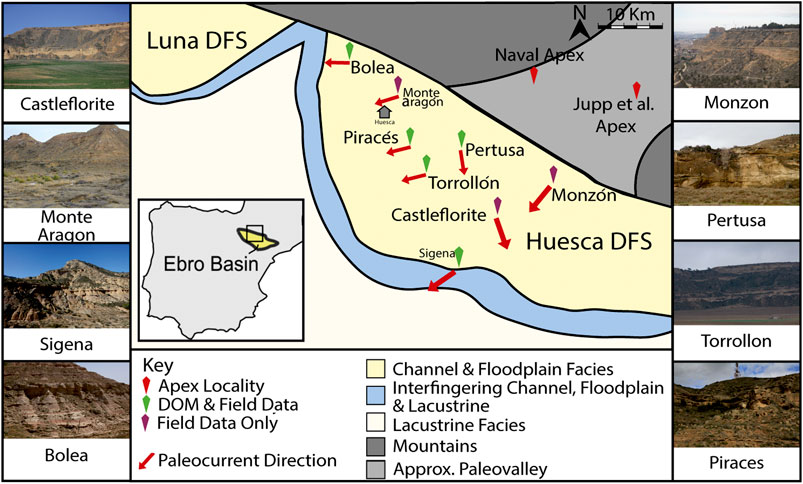
FIGURE 1. Location map showing the Ebro Basin. DOM = digital outcrop models. Position of two calculated apices (Naval and Jupp et al., 1987) are plotted (see text for discussion) as well as position of each study located. Facies map modified from Nichols (2017). See Supplementary Material for precise outcrop locations and orientations.

Within the basin, alluvial fan, fluvial fan and lacustrine systems have been recognized (e.g., Allen, 1983; Hirst and Nichols, 1986Nichols 1987; Hirst, 1991; Nichols and Hirst 1998; Arenas and Pardo, 2000; Nichols and Fisher, 2007; Hamer et al., 2007). On the northern margin, two major fluvial systems have been mapped, namely the Huesca and Luna DFS (Figure 1). In addition, a multitude of smaller alluvial fan deposits have also been mapped across the northern margin of the basin that interfinger with and occupy the area between the Luna and Huesca fluvial systems (Lloyd et al., 1998; Nichols and Hirst, 1998; Nichols, 2005). The Huesca system, the focus of this study, has been interpreted as a fan-shaped fluvial system with a radius of 60–70 km with south to south-westerly directed paleocurrents (Hirst, 1991). Deposits are part of the Sariñena Formation with fluvial channel sandstones, floodplain splay, paleosol and lacustrine deposits identified (Friend et al., 1979; Hirst, 1991; Donselaar and Schmidt, 2005; Hamer et al., 2007; Nichols & Fisher, 2007; van Toorenenburg et al., 2016). Downstream facies changes have been to some extent already quantified by Hirst (1991) whereby in channel percentage, lithological components (facies associations), proportion of ribbon sandstones and sandstone body thickness have been documented. The termination of the Huesca system is relatively well understood with interfingering of fluvial and lacustrine deposits reported (Hirst and Nichols, 1986; Hirst, 1991; Nichols and Hirst, 1998; Hamer et al., 2007; Nichols and Fisher, 2007). The interfingering of lacustrine and distal fluvial deposits is interpreted to represent seasonal alternations of lake level due to climatic changes (Nichols and Fisher, 2007). Gypsum and carbonates present within the center of the basin supports this inference suggesting periodic drying out of the lake (Nichols, 1987; Arenas and Pardo, 2000). This study aims to build upon this previous work by quantitatively detailing not only the downstream trends, but the vertical trends and lateral variations across the exposed portion of the Huesca DFS.

Methods

Eight localities were selected across the system based on outcrop quality and spatial coverage (Figure 1). At all localities, sedimentary logs were measured in the field at a decimeter scale and key information such as grain size, sorting, presence and size of sedimentary structures, paleocurrent data and storey surfaces presence. Sedimentary log location was chosen as the route that had the most accessible exposure within the outcrop belt. In addition, an architectural analysis was conducted using photo-panels so that channel geometry and stacking relationships could be determined. A facies analysis was conducted on the deposits adapting the scheme established by Miall (1985) as well as incorporating architectural element analysis (e.g., Miall, 1988; Owen et al., 2017a) to establish key facies, and sub-facies associations as well as determining deposit geometry.

Virtual outcrop models (VOM) were provided by the SAFARI consortium for five localities (see Figure 1) and were created from LiDAR datasets (Pertusa and Piracés; see Buckley et al., 2008 for methodology) and unmanned aerial vehicle (i.e., drone) datasets (Torrollón, Sigena and Bolea) (see Bemis et al., 2014 for methodology and review). Resolution within the VOM’s was sufficient (down to ∼20 cm) to identify floodplain and channel facies as well as internal characteristics (e.g., storey surfaces). Resolution was not sufficient for sedimentary structure identification. Virtual outcrop models were analyzed using the LIME Virtual Outcrop Geology (VOG) software (Buckley et al., 2019) where ‘pseudo’ sedimentary logs were measured, within which channel and floodplain facies were vertically mapped (e.g., Nesbit et al., 2018; Figure 2). Scree deposits were noted in the database and tentatively interpreted to be floodplain deposits based on exposure style and laterally adjacent deposits. VOM sizes vary from site to site; up to 2 km wide at Torrollón and down to ∼100 m wide at Pertusa. To ensure consistency across the different outcrop belts a 50 m interval was chosen. While this means more logs were measured at larger outcrops, it ensures that differences in sedimentary characteristics (e.g., channel percentage) is fairly analyzed across the system.

FIGURE 2

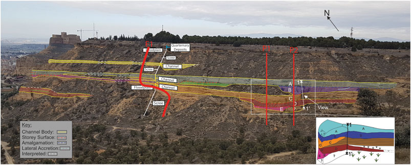
FIGURE 2. Outcrop image of Monzón, indicating how the variation in channel amalgamation can result in a high variance in channel percentage statistics, see P1 and P2 for two possible pseudo-log locations. Difference between pseudo-log path and field path (F1) is indicated. Note the field section route is dictated by accessibility while the pseudo-log location is not. Letters A–E represent different storey packages.

Statistical data (channel body thickness, channel percentage), collected from 1D sedimentary field logs and 1D ‘pseudo’ logs were plotted onto graphs and maps to allow for a quantified analysis whereby up-section and downstream trends were assessed across the system. Correlating outcrops across the Huesca is not easily achieved due to a lack of an appropriate marker across system. A broad correlation that places deposits relative to one-another by extrapolating the regional dip (see Section 5; Figure 3) was established. In addition, a weighted average grain size was calculated from field data alone by converting Wentworth nomenclature to phi, with the thickness of deposits weighting the averages to ensure an accurate representation of grain size distribution (see Owen et al., 2019). Where silts were noted within channel bodies, a grain size of 0.062 mm was used.

FIGURE 3

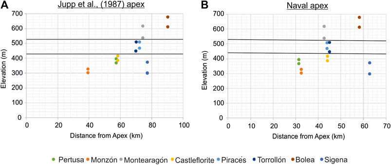
FIGURE 3. Graphs showing relative vertical position of each locality studied within the general stratigraphic column. Note dots depict the bottom and top of each sedimentary log. Black lines depict three broad stratigraphic horizons (see text for discussion). Left plot (A) shows the position of each locality studied from the calculated Jupp et al. (1987) apex. Right plot (B) the position of revised apex position (Naval) based on field observations and facies distributions.

Apex Estimation

Defining the position of an apex for any point-sourced depositional system (e.g., DFS, delta or submarine fan) is important when reconstructing the paleogeography of a specific system and also when determining downstream trends (Owen et al., 2015a; Owen et al., 2015b). Jupp et al. (1987) used a statistical method to project the position of an apex for the Luna and Huesca DFS using paleocurrent data, the von Mises distribution and the method of maximum likelihood. Although the apex for the nearby Luna DFS was well constrained, estimations for the Huesca DFS were much broader (Jupp et al., 1987). This can be attributed to either the Huesca DFS having a wide apex area, such as is observed on the modern Okavango DFS, or that there was insufficient paleocurrent data to predict its location as data were restricted to the western portion of the Huesca system.

Mapping of the feeder zone by Vincent and Elliott (1996) suggests that the Huesca fluvial system did have a wide apical area, with the town of Naval (located 32 km northwest of Jupp et al., 1987) located in the center of this zone where conglomerate deposits are thought to correlate with the Huesca system. To further test whether using Naval, or the apex position of Jupp et al. (1987) influences results, the distance to studied sites from each apex was plotted utilizing code published by Owen et al. (2015a). As can be seen in Figure 3, subtle differences do occur between the two different apices. Many locations experience a slight shift in relative position downstream depending on which apex is applied, for example Pertusa goes from being ∼56 km downstream using Jupp et al. (1987) to ∼34 km downstream using the Naval apex (Figure 3). Here we prefer the Naval apex estimation as it is more geologically consistent, based on architectural and sedimentary characteristics (see this paper) as well as the mapped conglomerates of Vincent and Elliott (1996), than that of Jupp et al. (1987). Therefore, the Naval apex is used as the point from which downstream distance is measured within this paper. Sites were then determined to be proximal, medial or distal using characteristics (e.g., channel stacking patterns and channel %) as defined by Nichols and Fisher (2007), Owen et al. (2015b) and Weissmann et al. (2015).

Seven facies have been defined and are summarized in Table 1. Collectively these facies, in conjunction with architectural analyses, imply deposition within two broad facies associations, namely floodplain and fluvial channel. Within the channel facies association, four sub facies associations have been identified (Table 2); 1) downstream accretion packages (DA) representing deposition from a braid bar (e.g., Smith, 1970; Miall, 1977; Bridge, 2003); 2) lateral accretion packages (LA), interpreted to be the deposits of point bars (e.g., Jackson et al., 1976; Friend et al., 1979; Miall, 1985); 3) undifferentiated channel fill (UC) which are interpreted to be barforms but a lack of paleocurrent indicators do not allow further interpretation; and 4) abandoned channel fill (AF) which represent the fine grained deposits once the channel has avulsed (e.g., Gagliano and Howard, 1984; Fisk, 1947; Hooke, 1995). Within the Floodplain facies association, three sub-facies associations are observed (Table 2); 1) Splay channels; 2) Splay sheets; and 3) Paleosols which demonstrate the post-depositional modification of deposits.

TABLE 1

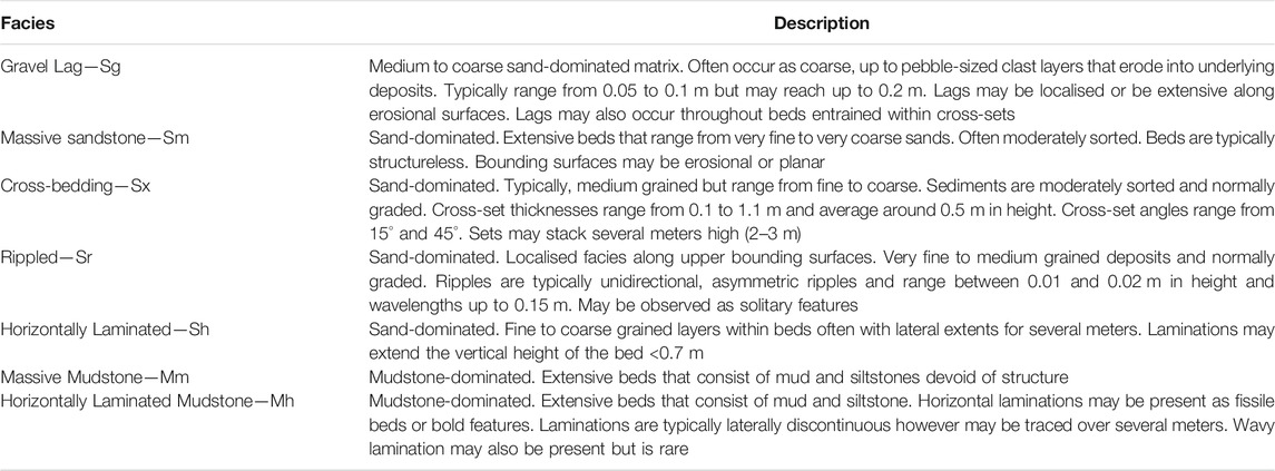
TABLE 1. Summary of facies.

TABLE 2

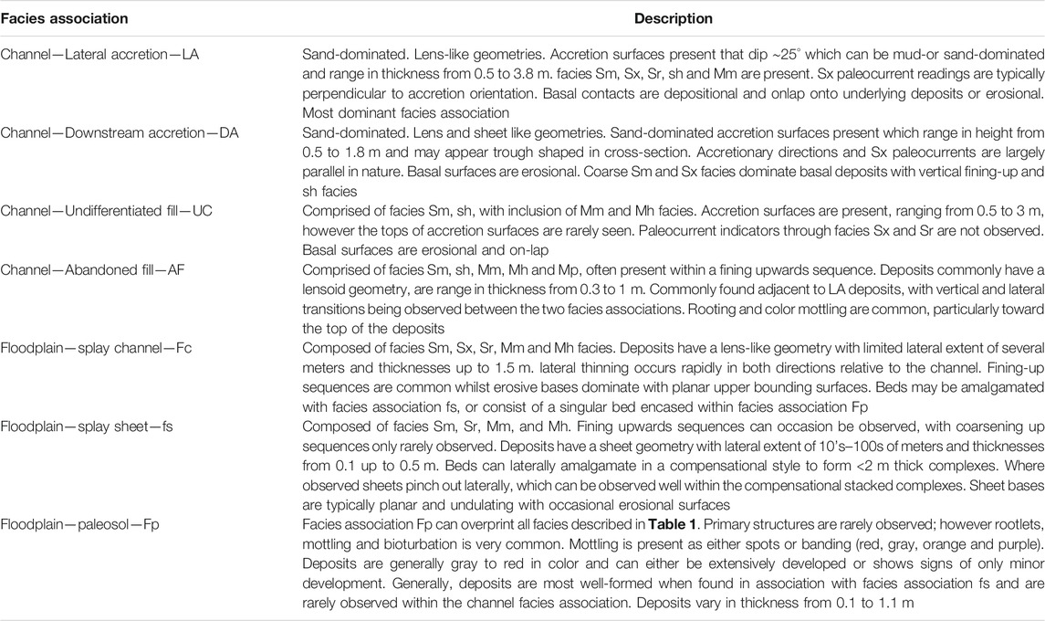
TABLE 2. Summary descriptions of facies and sub facies associations on the Huesca DFS.

Five sandstone channel body geometries are recognized within the Huesca fluvial system. The different sandstone body geometries are identified based on the scheme of Owen et al. (2017a) whereby traditional “sheet geometries” (c.f. Friend et al., 1979) are separated into distinctive sandstone body geometries based on external geometry and the internal relationship of storey surfaces (Owen et al., 2017b). Storey surfaces are defined as being the erosional base of active channels, that truncate previous channel deposits, within an overall channel belt (i.e., intra-channel belt surfaces, e.g., Friend et al., 1979). The five principal geometries include Massive (M), Semi-amalgamated (SA), Internally amalgamated (IA), Offset-stacked (OS) and Isolated (I). A summary of the different channel bodies is shown in Table 3 and Figure 4.

TABLE 3

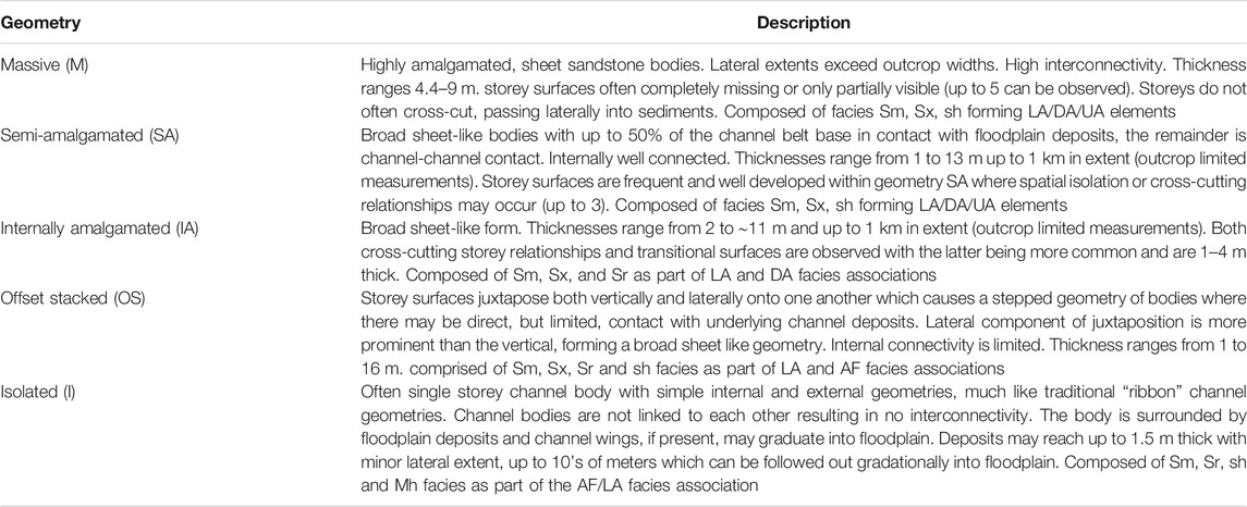
TABLE 3. Summary descriptions of channel body geometries observed on the Huesca DFS. See Figure 3 for example images.

FIGURE 4

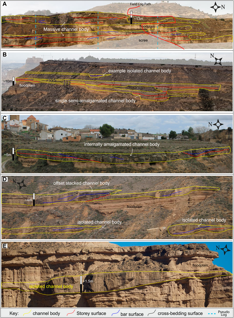
FIGURE 4. Example sandstone body geometries. (A) example of M geometry from Pertusa outcrop. Note the dominance of amalgamated channel body geometries. Note the difference in log location depending on whether it is field or Pseudo log based. (B) Example of SA and I geometry from Monzón. (C) Example of IA geometry from Pertusa. (D) Example of OS and I geometries from Castleflorite. (E) Example of I geometry from Castleflorite.

Vertical Trends

Observations

Within the Huesca DFS it is not possible to correlate precisely between sections due to a lack of age constraints and correlation datums. To help constrain the relationship between studied sections, elevation of the base and top of each section was taken as an approximate estimate of stratigraphic height. This assumes a uniform low dip (e.g., <2°) and a lack of faults between sections, which appears reasonable as all localities south of the Barbastro anticline (Martínez-Peña and Pocoví, 1988) show little or no deformation and there is no evidence for faults on geological maps (e.g., Teixell Cácharo and Garcia-Sansegundo, 1990). As can be seen in Figure 3, studied sections can lie at different stratigraphic heights. Bolea and Montearagón are relatively high in the stratigraphic column, with Torrollón and Pertusa being of near equal height. Castleflorite and Pertusa closely overlap with Monzón and Sigena being relatively low in the stratigraphic column. Figure 3 therefore highlights that it cannot be assumed that only spatial controls are relevant as the difference in stratigraphic height may mean that different conditions were present at different temporal periods. The data collected from the VOM and field sections fit well within typical characterizations of proximal, medial and distal settings meaning that whilst we are unable to determine definite ages of the strata, the data is relevant when examining channel percentage, vertical trends and grain size for these positions within DFS.

To decipher whether vertical trends exist within the study area, channel body thickness and geometry was plotted against height in succession so that insights into fluvial system behavior could be gained through time (e.g., Owen et al., 2019; Wang et al., 2011). Small scale trends were determined using Spearman’s rank correlation coefficient (ρ), coefficient of variance (CV) and moving averages for each succession to allow for direct comparison with other published works (e.g., Owen et al., 2019). Successions were grouped using ρ values; the first showing weak or no relationship (± <0.19); the second with a weak relationship (±0.2–0.39); group three is a moderate relationship (±0.4–0.59); group four a strong relationship (±0.6–0.79); group five a very strong relationship (±0.8–1). We acknowledge that some sections have a low quantity of data points (namely Sigena, and Bolea) however this is due to the scarcity of channels in this portion of the system.

The results (Figure 5) show a mixture of strong to weak or no relationship of vertical trends within the studied sections. In the most proximal settings (Pertusa and Monzón), very strong to strong relationships are observed in which channel body thickness generally increases up-section. Strong relationships are also observed in the most distal sections with Bolea demonstrating an up-section increase (ρ = 1) (although n = 2 due to its distal locality) and Sigena in which an up-section decrease in channel thickness is observed (n = 4 due to its distal locality; ρ = −0.6). At these two localities, differences in channel body thickness are minimal compared to other sections, and visually represent consistent channel body thicknesses up-section. All other sections, largely located within the medial portion of the system, show weak to no up-section trends in which channel body thickness varies considerably up-section in a non-systematic manner.

FIGURE 5

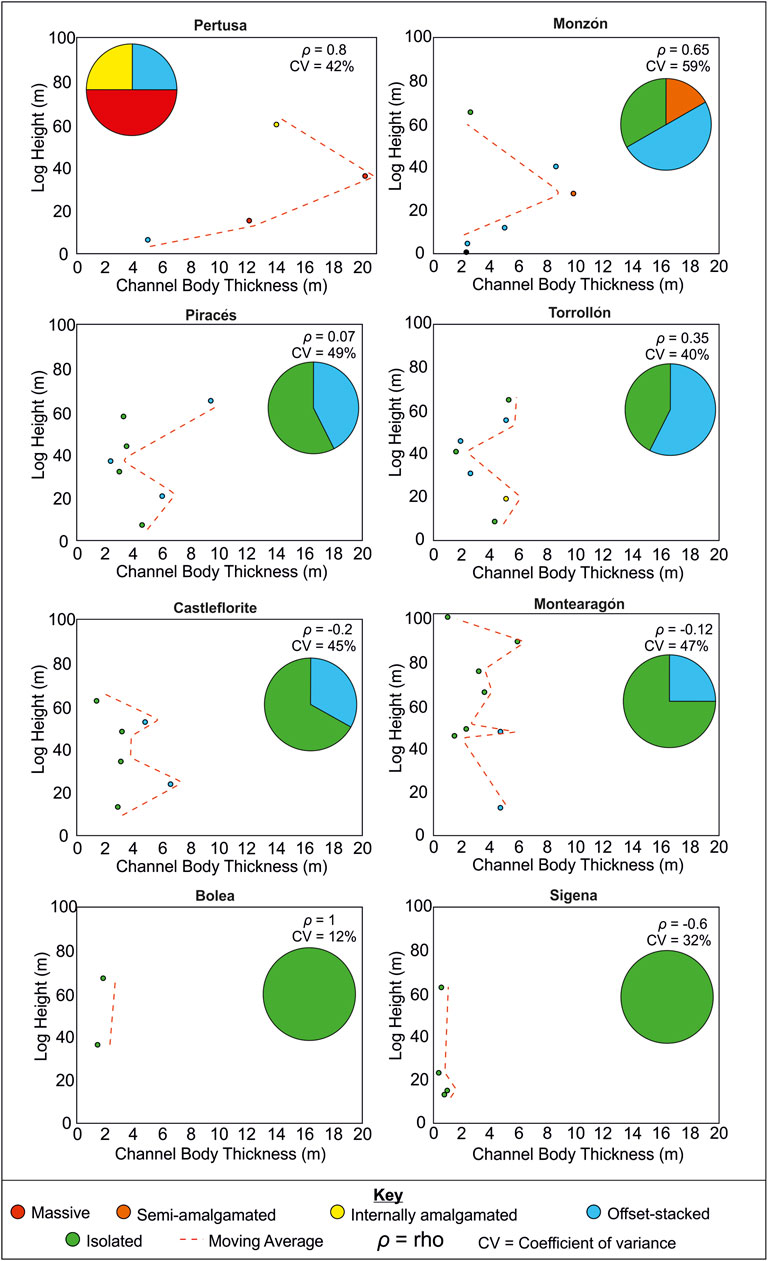
FIGURE 5. Log height of channel body against channel body thickness for each succession studied. Colored dots represent the interpreted channel geometry present. Moving averages, ϱ and CV are noted for each succession. The pie chart breakdown shows the percentage of channel body geometry types for each locality.

Based on the assumptions that fault activity has not displaced sequences (as indicated by local geology maps), the studied locations can be broadly grouped based on their near equal stratigraphic height. Monzón, Sigena, Pertusa and Castleflorite all overlap at the base of the stratigraphy. Monzón and Pertusa display increases in channel body up-section, while Sigena and Castleflorite show no up-section trends. Torrollón and Piracés broadly correlate stratigraphically with one-another and exhibit no up-stream trends. At the top of the stratigraphy, Montearagón and Bolea overlap and only Bolea displays an up-section increase in channel thickness. This shows that no pattern is dominant within a particular portion of the stratigraphy suggesting that, at the larger stratigraphic scale, the fluvial system was not undergoing any significant systematic changes through time.

Discussion of Vertical Trends

Up-section changes in channel body thickness have been interpreted to represent the progradation or retrogradation of the system (e.g., Kjemperud et al., 2008; Weissmann et al., 2013; Rittersbacher et al., 2014; Owen et al., 2017b; Owen et al., 2019 and Wang et al., 2011, among others). The above analysis demonstrates that at the local level there were variations in fluvial behavior, and likely represent autocyclic variations and an interplay between sediment supply, discharge regime, avulsion rate and frequency and local subsidence differences (e.g., Shanley and McCabe, 1994; Posamentier and Allen, 1999; Holbrook et al., 2006, see Owen et al., 2019 for detailed discussion). The most proximal locations (Pertusa and Monzón) exhibit progradational up-section trends, likely the response to increases in sediment supply which is closest to the sediment source (e.g., Owen et al., 2019; Wang et al., 2011). The variability observed at the medial sections (Piracés, Torrollón, Castleflorite) suggest the characteristics of avulsion cycles varied more in comparison to other areas. Distal localities (Montearagón, Bolea, and Sigena) display more simple vertical profiles in which minor changes in channel body thickness are observed with simple aggrading patterns. The lack of observable trends in different portions of the DFS, as well as the overall stratigraphy, suggest that a system wide allocyclic trend (e.g., progradation or retrogradation) is not present in the exposed portion of the stratigraphy that is being analyzed. The discrepancies in trends across the sections are interpreted to be the result of smaller scale autogenic noise related to avulsion process and small-scale fluctuations in sediment supply (e.g., Hajek et al., 2010; Wang et al., 2011; Rittersbacher et al., 2014; Owen et al., 2017a; Wang et al., 2011).

Spatial Trends

Channel Geometry

Channel body geometry clearly changes in a downstream transect on the Huesca DFS. As can be seen in Figure 5, the most amalgamated, complex geometries are found in proximal localities where Pertusa is the only locality with geometry M and IA present, and Monzón is the only locality at which SA is observed. Geometry OS is observed across the system, being most prevalent in medial localities (Figure 5; e.g., Monzón, Torrollón). Geometry I is found across the system, but dominates successions in the distal portions of the system (e.g., Bolea and Signena; Figure 5). Montearagón however, despite being medial in terms of distance downstream, is dominated by distal channel geometries (I and minor OS).

Channel Body Percentage

Channel body percentages were calculated from both field and pseudo-logs. Field data indicate channel body deposits made up a total of 36% of all sediments logged across the system, although channel percentages within individual successions range from 66 to 4%. When considering both the field and pseudo-log data, channel deposits make up 27.5% (averages range from 71 to 4%) of all logged sediments, a notable difference of −8.5% from field data alone.

Data from field logs (Figure 6A), shows that channel body percentage overall decreases downstream with the highest values residing in the most proximal locations (e.g., 70% at Pertusa) and lowest in the distal (e.g., 4% at Sigena) However, variability is observed in the medial successions where a systematic decrease is not observed (ranging from 44 to 31%). Interestingly, of the medial successions, Montearagón has one of the lowest channel percentages (26%) despite being the closest medial section to the estimated apex.

FIGURE 6

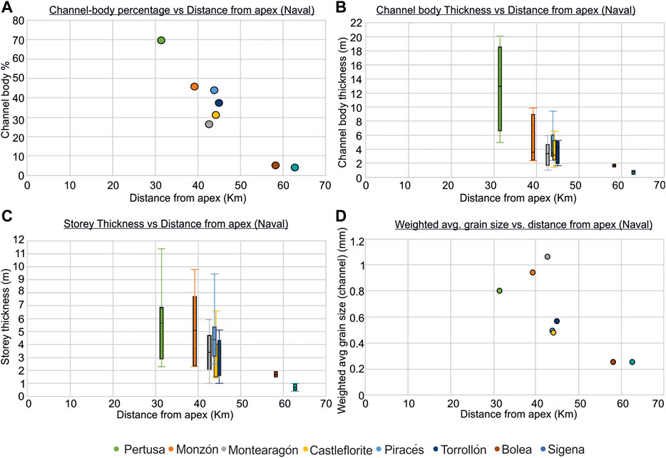
FIGURE 6. Spatial trends on the Huesca DFS. The Naval apex location has been used to depict distance downstream. (A) Channel body percentage vs. distance downstream. (B) Channel body thickness vs. distance downstream. The data are represented as box and whisker plots. (C) Storey thickness v distance downstream. The data are represented as box and whisker plots. (D) Weighted average grain size vs. distance downstream.

When considering the pseudo-log dataset, similar trends can be seen (Figure 7A). Pertusa (most proximal locality) has an average channel percentage of 71% with a range of ∼10% observed. Similarly, the lowest channel percentages are observed in the most distal section (e.g., Sigena) with an average of 7% and range of ∼15%. Interestingly medial sections have the largest range with a range of 32% (Piracés) and 37% (Torrollón) observed. Bolea again, despite being the closest medial site to the apex, has an average channel percentage of 4% which is more diagnostic of distal deposits.

FIGURE 7

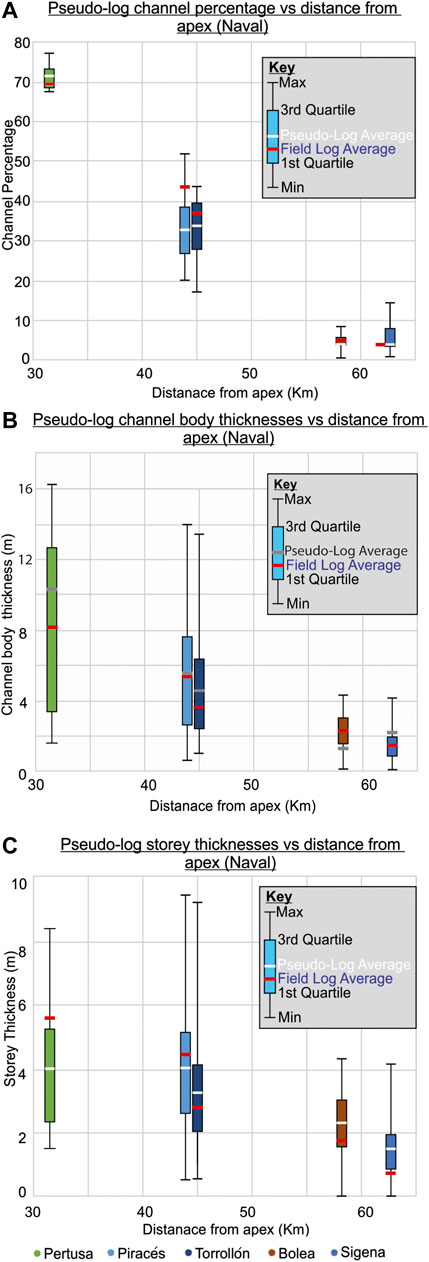
FIGURE 7. Spatial trends present for data collected from virtual outcrop models (pseudo-logs). The average from field logs is noted for comparison on each box and whisker plot. (A) Calculated channel percentage from virtual outcrop models vs. distance downstream. (B) Calculated channel body thickness from virtual outcrop models vs. distance downstream. (C) Calculated storey thickness vs. distance downstream.

Channel Body Thickness

When considering the field dataset, a large range in channel body thicknesses is observed, from 0.4 to 20.2 m across the system (Figure 6B). Average channel body thicknesses range from 0.7 to 13.1 m across the system, with the highest averages observed in the most proximal localities (13.1 m at Pertusa) and the lowest in the most distal localities (0.7 m at Sigena and 1.7 m at Bolea). As with the channel body percentage dataset, the medial sections do not show a systematic decrease in average channel body thickness but they do however group together on the plot with averages ranging from 4.3 to 3.5 m (Figure 6B). Although typically the largest maximum thicknesses are observed in the proximal reaches and the smallest in the distal reaches, there is a large degree of overlap in channel body thicknesses overall. For example, maximum thicknesses in distal localities almost overlap with minimums from proximal localities (Figure 6B). This suggests that a particular sandstone body thickness is not indicative of being either proximal, medial or distal, unless within the extreme ends of measured thicknesses.

Similar trends can be seen within the pseudo-log dataset (Figure 7B). The thickest average is found in the most proximal site (8.2 m at Pertusa) while the thinnest average channel body size is at Sigena (1.5 m). Average channel body thicknesses in the medial zone are 5.6 m (Piracés) and 6.4 m (Torrollón). Again, an overlap in data is observed across the system, indicating no particular reading is indicative of a particular zone, however, the thickest bodies are generally observed in the most proximal region, and thinnest in the most distal. The largest range in channel body thicknesses are in the most proximal region, with the range reducing downstream.

Storey Thickness

Storey thicknesses can provide important information on the erosional capabilities of fluvial channels on the Huesca DFS, although it should be noted that cross-cutting relationships often mean that full storey thicknesses are not preserved. From field data, storey thicknesses within the Huesca DFS range from 0.4 to 11.4 m with average thicknesses ranging from 0.7 to 11.4 m (Figure 6C). As with other datasets, there is an overall decrease in storey thickness downstream within the Huesca fluvial system. The largest storey average is found at the most proximal location (5.7 m at Pertusa) while the thinnest at Sigena (0.7 m). Medial sites have average storey thickness that fall within 4.6 m (Piracés) to 2.9 m (Torrollón). There is an even greater degree of overlap in the storey thickness dataset compared to other datasets due to the smaller values involved. As with the channel body thickness dataset, no measured thickness is indicative of being either proximal, medial, or distal, with the exceptions of maximum thicknesses giving an indication of location within the DFS.

Interestingly, the range in storey thicknesses is smaller in the VOM dataset with storeys ranging in thickness from 9.46 to 0.53 m (a range of 8.93 m compared to 10.7 m for the field-based dataset) (Figure 7C). The largest average is in fact recorded at Piracés (4.07 m) rather than Pertusa (4.06 m), the most proximal locality. However, the difference (10 cm) is minimal. As in line with all other datasets, the smallest averages are found at the most distal localities (2.31 m at Bolea and 1.46 m Sigena).

Channel Grain Size

A weighted channel grain size analysis was conducted on the channel deposits. A downstream trend of decreasing channel body grain size is observed in the Huesca DFS with three groups which fit into DFS positions of proximal, medial and distal (Figure 6D). Interestingly, there are two notable outliers to the overall downstream trend. Montearagón has the coarsest grain size (coarse sand) yet sits at similar basinward distances as medial localities (Torrollón and Piracés). Monzón is coarser (0.939 coarse to very coarse sand) than Pertusa (0.83 mm, coarse sand) yet is located further basinwards from the apex (Figure 6D). A grouping of grain sizes ranging from medium to coarse sand (0.479–0.567 mm) is observed in medial sections (Piracés, Torrollón and Castleflorite), with distal localities being notably finer (fine to medium sand; 0.25 mm) than all other localities (Figure 6D).

In summary, the proximal region shows a low variance in channel body percentage, but a wide range in channel body thicknesses. Medial sections show wide range in both channel body thickness and presence while distal sections have a lower degree of channel percentage variance and thickness. It should be noted that with increasing distance, the difference between the calculated averages from the field and pseudo-log channel thicknesses also increases. The above analyses show that there are clear downstream trends within the Huesca DFS, an observation that is in line with the work of Hirst (1991).

Discussion

Downstream Trends

The Huesca fluvial system displays downstream trends clearly indicative of a distributive fluvial system. Radial paleocurrents were noted in Hirst (1991) with further paleocurrent data collected within this study supporting observations (Figure 1). Field observations from this study found downstream decreases in channel body percentage (66.1–3.9%; decrease of 94%), channel body thickness (20.2–0.4 m; 98% decrease), storey thickness (5.4–1.7 m; 68% decrease), channel grain size (1.06–0.25 mm; 76.4% decrease) and a shift in channel body geometries from M dominated in the proximal system to OS-I dominated in the distal regions recorded. These data support the previous work of Hirst (1991), who first described the system as a fluvial fan and fits with the characteristics of a distributive fluvial system as suggested by Weissman et al. (2010) and Weissman et al. (2015). While confirming these observations, this paper provides additional quantification of the characteristics and variability within a DFS in a downstream transect as well as analyze vertical trends.

Downstream trends are attributed to a downstream decrease in stream power as a function of channel avulsion and bifurcation alongside infiltration and evaporation processes (e.g., Weissman et al., 2010, Weissman et al., 2015). A decrease in transport capacity away from the apex of the system, coupled with a wider surface area for the system to migrate and build stratigraphy over, impacts the development of thick, amalgamated channel bodies and leads to the formation and preservation of thinner, sheet channel bodies separated by extensive floodplain packages leading to isolated single storey bodies in the distal realm. As the basin was endorheic, base-level changes are considered to have little impact on the development of the overall DFS unlike their marine connected counterparts (e.g., Fisher and Nichols, 2013). However, fluctuating ephemeral lake levels in the distal area may have played a minor role in altering development in the distal region, but are perceived to have aggraded in line with the fluvial system (Fisher and Nichols, 2013). From these observations, we can determine that the Huesca fluvial system was primarily influenced by upstream changes in sediment supply and stream power (e.g., Kukulski et al., 2013).

Montearagón is a consistent outlier within the weighted average channel grain size (relatively high), channel percentage (relatively low at 20%), and dominant geometry (I) for its position on the DFS when compared to basin center counterparts. With respect to downstream distance this location is considered to be the most proximal medial locality, yet all the characteristics observed at this locality suggest it is a distal DFS locality. What must be considered is that whilst the distance from the estimated apex is comparable to the other medial localities (e.g., Piracés, Torrollón, Castleflorite), Montearagón is in a basin margin location, rather than basin center. The low channel percentage may be because the river would have to avulse to nearly 90° to deliver sediment to this area of the DFS, whereas the basin center counterparts lie within the axial thoroughfare of the system. It is considered more likely to avulse within these localities, and only in extreme cases (i.e., super elevation of lobes in the central axial portion of the system) occupy basin margin locations. The coarse grain size may be the function of basin margin alluvial fans acting as tributary networks, or interfingering with the Huesca system, intermittently supplying coarse sediment to the locality. Field observations suggest the sediment is relatively immature compared to others with more noticeable angularity to the coarser grains. These observations suggest that while downstream trends are apparent on DFS, they are not clear concentric radial patterns from basin margin to center.

Lateral Variability

While previous DFS models have been produced from individual log sections across a system (e.g., Owen et al., 2015b), the use of virtual outcrop models has been implemented within this study to better understand how channel body presence varies laterally across individual and several outcrops within a single system. This approach provides a better understanding of net: gross (in this case channel and floodplain facies) variation across outcrops thus allowing a better understanding of how consistent characteristics are across and within the different zones (proximal, medial and distal) in a DFS. Our data show that whilst the proximal and distal zones show reasonably consistent channel percentages, large variations can be present within single outcrops in the medial zone. For example, at Piracés and Torrollón based on Pseudo log data, channel percentage can vary by 32 and 27% respectively. However, at Pertusa (relatively proximal) only 10% is observed and Bolea and Sigena (relatively distal) 9–15% is observed. Across the whole medial section channel percentage can vary from 15 to 52%. Although within our dataset this does not overlap with readings within the distal and proximal sections, the reported maxima and minima could be interpreted to be proximal, or distal, deposits. Rittersbacher et al. (2014) also found through the creation of ‘pseudo-logs’ within a large outcrop in the Cretaceous Book Cliffs, a large degree of lateral variation (ranging from 23–58% channel sand percentage) in their study of medial Blackhawk Formation deposits. Similarly, Führ Dal’ Bó et al., (2018) note that medial deposits in the Upper Cretaceous Marília Formation, SE Brazil, show significant variation in net channel to floodplain ratios.

The large degree of variation in channel proportion within the medial portion of a DFS is interpreted to be due to varying degree of channel amalgamation. In the medial region of a DFS channel body deposits become increasingly vertically separated by floodplain packages. However, channel bodies are not consistently, or fully, separated by floodplain packages as some channel bodies may be amalgamated in places. As a result, the pseudo-logs capture this variation in degree of amalgamation, showing that whilst an increase in accommodation is observed, it is not sufficient to consistently separate channel body deposits with floodplain deposits. This can be observed in Figure 2 by comparing log P1 with log P2. The small degree of variation observed within the proximal realm is due to logs sampling sporadic floodplain packages, while in the distal realm it is entirely dependent on whether the log intersects the sparse channel bodies. As a result, the difference between a 4-5 storey channel body and capturing the wing of a channel body can greatly affect the channel body to floodplain ratio in the medial realm, while floodplain and channel deposits are only present in minor amounts in the respectively proximal and distal realms, and thus will not vastly influence the percentages. The medial zone is consequently a zone of high variability and will require further work to characterize and understand the controls on this variability, particularly as net: gross (i.e., channel body percentage vs. floodplain percentage) can vary greatly both with respect to lateral and vertical connectivity.

A high degree of variability is also observed in the channel body and storey thickness dataset. As with the channel percentage dataset, downstream trends are still apparent, but even more overlap is observed (Figures 6 and 7). Interestingly the proximal region shows the most variability for the channel body dataset, becoming less variable downstream. Storey thickness is variable in both the proximal and medial settings, varying the most in the proximal setting using field data (Figure 6) but most in the medial area in the pseudo-log dataset (Figure 7), however the ranges between these two datasets are very similar (9.12 and 8.96 m respectively). Soares et al. (2018) found that proximal parts of a DFS in the Barau Basin, Brazil, recorded high frequency stacking patterns of channel deposits within an overall sedimentary cycle and attribute this to high frequency, short term changes in climate. Sediment supply in the Ebro Basin is expected to have fluctuated in relation to active tectonics within the Pyrenean orogenic belt. We envisage that a combination of such controls, would have driven variations in discharge and sediment supply ultimately resulting in the large degree of channel body and storey thicknesses observed in the proximal setting of the Huesca DFS. However, these fluctuations were not long lived to produce either a prograding, or retrograding stratigraphy but rather short-lived variations. When fluctuations are encountered, the river system in the proximal area will aggrade, migrate, or incise as the river redistributes and transports the sediment as it enters the sedimentary basin (e.g., Weissmann et al., 2013; Weissmann et al., 2015). In comparison to the rest of the system, the proximal portion will encounter more frequent avulsions as the system builds stratigraphy over a smaller area. This will result in varying degrees of reworking rates, and therefore thicknesses in both storey and channel body thicknesses. Further downstream, the impact of changes in sediment supply and discharge variations are less due to increasing distance from the source (apex) area, which in the Huesca DFS appears to be beyond the outcrop belts of Torrollón and Piracés (where storey thickness ranges are still high; see Figures 6 and 7). There appears to be no preservation of large scale climatic and tectonic processes within the vertical logs dataset, however it is recognized that such signals may be ‘shredded’ (e.g., Jerolmack and Paola., 2010; Straub et al., 2020).

Our data indicate that there is a significant degree of variation in channel percentage, and channel body and storey thicknesses across the Huesca DFS, however, these variations occur within a clear overall decreasing downstream trend. It is important therefore to not infer position on a DFS without multiple datapoints due to the large degree of variation present, particularly in the medial area. Our data also suggest that when inferring position on a DFS the best indicator to use is channel body architecture, and if this is not available (i.e., as in many subsurface datasets), that channel body percentage should be used. It is likely that these datasets are the best to form generic models as they are not dependent on fluvial, and channel, sizes which varies across DFS (e.g., Hartley et al., 2010b; Weissmann et al., 2010). The data presented here help to better refine the understanding of the DFS model, specifically where channel percentage, and consequently net:gross, varies laterally, as is summarized in Figure 8. The data will aid resource exploration in the oil and gas sector, but also with respect to better understanding the distribution of aquifer prone sands. This may allow for better understanding in stressed environments, such as those documented in India, where water resource availability and management is a pressing issue, particularly with the respect to understanding pollutant pathways (e.g., Mukherjee et al., 2015; MacDonald et al., 2016; Bhanja et al., 2017). It is also important to note that both the virtual outcrop and field-based datasets are still limited to some extent by exposure quality. This must be considered when comparing statistics gained within this study to those that are subsurface based where finer grained material (e.g., floodplain deposits) can be more fully examined.

FIGURE 8

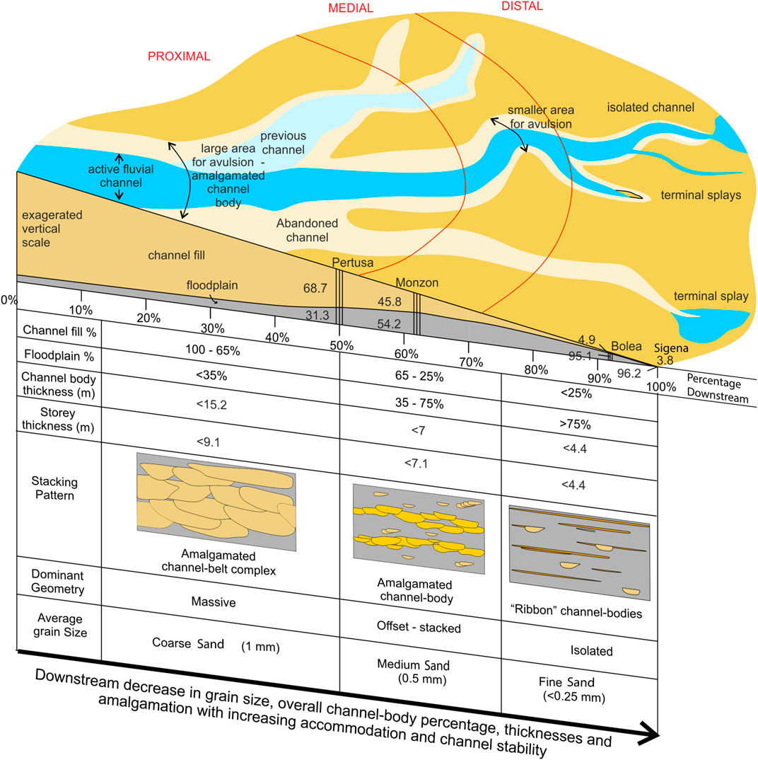
FIGURE 8. Summary diagram of the variability observed in the Huesca DFS. Note statistics shown are a combination of field and virtual outcrop model data. Proximal, medial and distal zones are defined based on sedimentary characteristics (see text). X axis of the DFS represent percentage distance downstream (normalized distance downstream).

Field Data v Pseudo-log Data

It is often the case with field-based data collection that log location is chosen based on a delicate interplay between outcrop accessibility and exposure quality. Virtual outcrop models provide a solution to collecting data from inaccessible areas where specialist equipment would be required for the safe collection of data in the field. As a result, straight vertical log locations can be chosen, which is uncommon in the field as the landscape and terrain is navigated. It is clear from our study that vast amounts of data can be collected from virtual outcrop models which helps feed much needed quantified data into modeling efforts (e.g., Bellian and Jennette., 2005; Fabuel-Perez et al., 2010) and build quantified predictive models. The VOM dataset therefore gives a better perspective of the variation in characteristics (e.g., channel thickness or percentage across an outcrop belt) compared to field-based datasets which are generally generated from more sparsely populated datasets.

Overall, when comparing the statistics obtained from field data and VOMs the same downstream trends are observed (Figure 9). Although more data were able to be acquired using the VOM method, the statistics fall broadly in line with one-another at a system scale. Figure 7A shows channel percentage data from VOM with actual field log values noted. The field log data generally falls within the 1^st and 3^rd quartiles with outliers of this trend present at Piracés and Pertusa. Figure 9A shows the difference in values obtained from each dataset. The highest variance between the pseudo-log average and field log actual is observed at Piracés (+11%) and the lowest variance observed at Bolea (+0.87%). Piracés is thought to have the highest variance as the different VOM intersect large channel bodies at different points (e.g., varying from the fringe to central channel body locations). The downstream trend of decreasing channel body percentage with increasing distance is the same within both the pseudo-log and field datasets with a stronger correlation observed within the field log dataset (Figure 9A: Field R² = 0.935; Pseudo R² = 0.841). This is because there is more variance in the VOM dataset due to its greater size, and Piracés pseudo-log reading pulling the average down.

FIGURE 9

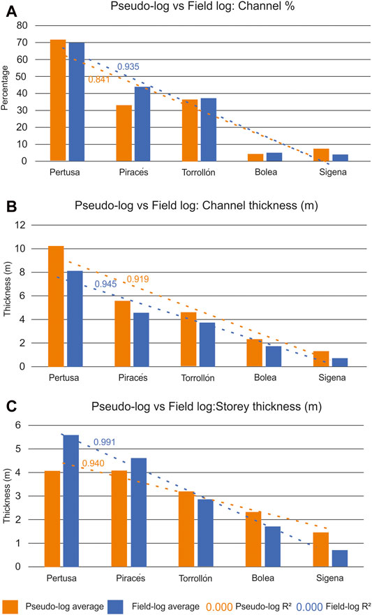
FIGURE 9. Graphs showing difference between Pseudo log v field datasets. (A) Comparison between average channel percentage from Pseudo log data and channel percentage calculated from field logs. (B) Comparison between average channel body thickness from Pseudo log data and average channel body thickness calculated from field logs. (C) Comparison between average storey thickness from Pseudo log data and average storey thickness calculated from field logs.

Within the channel body thickness dataset, VOM average measurements were consistently thicker than data from field logs (Figure 9B). The largest difference is observed in the most proximal settings with field-based averages (8.1 m) being 2.09 m thinner than averages from VOM datasets (10.19 m) (Figure 9B). This is due to VOM measurements being able to better measure large cliff style exposures (which often dominate proximal regions) in comparison to standard logging equipment in the field. Nonetheless, field log averages all fall within the 1st and 3rd quartiles of the VOM dataset (Figure 7B) except for Sigena where the field log average falls just outside the 1st quartile of VOM data. Overall, the same downstream trends are observed with both datasets with an overall decrease in channel body thickness with increasing distance, though this correlation is marginally higher within the field data than in the pseudo-log data (Figure 9B; Field R² = 0.945; pseudo-log R² = 0.919).

Storey thickness trends are similar in both the pseudo-log and field-based dataset with a general downstream decrease in storey thickness observed (Figure 9C). However, unlike with the channel body dataset, no dataset is consistently thicker than the other, with larger average values observed at Pertusa and Piracés in the field log dataset, while averages were thinner in the field dataset at Torrollón, Sigena and Bolea. Notably, the average storey thickness from field data are 50% thinner at Sigena. Therefore, relatively speaking a larger variance is observed in the storey dataset compared to the channel body dataset, although it must be noted that the range is much reduced. The R² is higher for the pseudo-log dataset (Field = R² = 0.991; pseudo-log R² = 0.940; Figure 9C).

Rittersbacher et al. (2014), from a study of a single large outcrop belt, similarly noted a greater variability in channel percentage (25%) in VOM generated datasets compared to field datasets, with the field based channel percentage falling within the middle of the range of the VOM dataset. In a study that focused on mapping meander belts in Dinosaur Provincial Park (Canada) Nesbit et al. (2018) report an average absolute difference between digital based facies and field-based facies of ±4.9% with a maximum discrepancy of 13.6%.

Although broad trends are similar the above analysis shows there is variability between the two datasets. It can be argued that the VOM derived datasets can provide a better representation of the variability present as the dataset has greater spatial coverage and true thickness measurements. In addition, truly vertical logs are easier to measure using the VOM, particularly in cliff exposure styles, when compared to field-based scenario in which accessibility issues can be present (as demonstrated when comparing field v pseudo-log location in Figures 2 and 4A). Although VOM resolution is lower than a field-based scenario, the variation between the two datasets is larger than the resolution limitations of the VOM. However, this study would not have been able to be conducted without initial field validation of facies present. Despite the increase in the quality of virtual outcrop model imagery over recent years, field data collection is still critical to gain information that cannot be gained from digital outcrop datasets alone. There is always a tradeoff between model size and quality (e.g., Buckley et al., 2008) but even with the highest resolution datasets, information on grain size and sedimentary structures can rarely be obtained in conjunction with larger scale stratigraphic stacking patterns. Without field based sedimentary logs and observations a proper facies analysis cannot be conducted. We therefore recommend the two data collection methods be done in conjunction with one-another. As this study highlights the wealth of information that can be gained when field and VOM datasets are used in conjunction with one-another, a greater understanding of variability in sedimentary characteristics at single outcrop belts to system scale scenarios can be achieved, thus allowing for more refined and robust predictive quantitative models. In this respect the virtual outcrop-based dataset is a substantial additional complimentary dataset to field-based analysis, allowing the outcrops to be further analyzed in a digital based environment (Buckley et al., 2008).

Conclusion

Our results show that there are clear overall proximal-distal trends within the Huesca distributive fluvial system, however internal variations exist. Data show that channel body and storey thicknesses and frequency, grain size and channel percentage decrease downstream. These observations agree with, and build upon, the initial work undertaken by Hirst (1991). However, in addition this study quantified vertical and lateral trends across the system at selected points downstream. Vertical trend analysis indicates that there is no overall temporal change in the nature of the fluvial system at the stratigraphic scale, but at the local scale the upward thickening and thinning of channel deposits is interpreted as autogenically driven “noise”. Although downstream trends are apparent, there is clear variability within the system with regards to storey and channel body thickness, as well as channel percentage which is particularly highlighted in the pseudo-log derived dataset. Channel body thickness is most variable in the proximal region, becoming less variable downstream, whereas channel percentage was most variable in the medial portion of the system. Storey thickness was found to be variable in both proximal and medial settings. Our study conforms with published DFS models but highlights important variabilities that must be taken into consideration when interpreting and exploring DFS deposits. In addition, we examined the similarities and differences between field based and digital based analysis of sedimentary outcrops. The VOM dataset gave a better representation of the variations observed at both outcrop and system scale in key characteristics in comparison to field derived datasets. This has important implications for understanding heterogeneity within DFS, particularly in areas of low data availability (e.g., subsurface datasets).

Data Availability Statement

The raw data supporting the conclusions of this article will be made available by the authors, without undue reservation.

Author Contributions

BM collected the field data and compiled the report alongside completing data analysis. AO acted as field assistant, aided in writing the paper. GN provided guidance and helped to edit and review the paper pre-submission. AH provided guidance and helped to edit and review the paper pre-submission. RW provided guidance and helped to edit and review the paper pre-submission. All authors contributed to the conceptualisation of the research idea.

Conflict of Interest

The authors declare that the research was conducted in the absence of any commercial or financial relationships that could be construed as a potential conflict of interest.

Acknowledgments

Author Ben Martin thanks the University of Glasgow for providing funding for this project through the ‘Stressed Environments’ scholarship fund. The SAFARI consortium (https://safaridb.com/home) are thanked for providing virtual outcrop models that have been analyzed within this paper. Two anonymous reviewers are thanked for their thorough and constructive comments on this paper.

Supplementary Material

The Supplementary Material for this article can be found online at: https://www.frontiersin.org/articles/10.3389/feart.2020.564017/full#supplementary-material.

References

Allen, J. R. L. (1983). Studies in fluviatile sedimentation: bars, bar-complexes and sandstone sheets (low-sinuoisty braided streams) in the Brownstones (L. Devonian) Welsh Borders. Sediment. Geol. 33, 237–293.

CrossRef Full Text | Google Scholar

Alonso-Zarza, A. M., and Calvo, J. P. (2000). Palustrine sedimentation in an episodically subsiding basin: the Miocene of the northern Teruel Graben (Spain). Palaeogeography Palaeoclimatology Palaeoecology 160, 1–21.

CrossRef Full Text | Google Scholar

Álvarez Sierra, M. A., Daams, R., Lacomba, J. I., López Martínez, N., van der Meulen, A. J., and Sesé, C. (1990). Palaeontology and biostratigrpahy (micromammals) of the continental Oligocene-Micoene deposits of the North-Central Ebro Basin (Huesca). Scripta Geologica 94, 1–75.

CrossRef Full Text | Google Scholar

Arenas, C., and Pardo, G. (2000). Neogene lacustrine deposits of the north-Cantral Ebro Basin, Northeastern Spain, lake basins through space and time. AAPG Stud. Geol. 46, 395–405.

Google Scholar

Barberá, X., Cabrera, L., Marzo, M., Parés, J. M., and Agustí, J. (2001). A complete terrestrial Oligocene magnetobiostratigraphy from the Ebro Basin, Spain. Earth Plan. Sci. Lett. 187, 1–16.

CrossRef Full Text | Google Scholar

Bellian, J. A., and Jemmette, (2005). Digital outcrop models: applications of terrestrial lidar technology in stratigraphic modelling. J. Sediment. Res. 75, 176. doi:10.2110/jsr.2005.013.166

CrossRef Full Text | Google Scholar

Bemis, S. P., Micklethwaite, S., Turner, D., James, M. R., Akciz, S., Thiele, S. T., et al. (2014). Ground-based and UAV-based photogrammetry : a multi-scale , high-resolution mapping tool for structural geology and paleoseismology. J. Struct. Geol. 69, 163–178. doi:10.1016/j.jsg.2014.10.007

CrossRef Full Text | Google Scholar

Bhanja, S. N., Mukherjee, A., Rodell, M., Wada, Yoshihide, W., Chattopadhyay, S., et al. (2017). Groundwater rejuvenation in parts of India influenced by water-policy change implementation. Sci. Rep. 7 (1), 7453.

Google Scholar

Bridge, J. S. (2003). Rivers and floodplains. Forms processes and sedimentary record. Oxford, United Kingdom: Blackwell Publishing Ltd.

Google Scholar

Buckley, S. J., Howell, J. A., Enge, H. D., and Kurx, T. H. (2008). Terrestrial laser scanning in geology: data acquisition, processing and accuracy considerations. J. Geol. Soc. 165, 625–638. doi:10.1144/0016-76492007-100

CrossRef Full Text | Google Scholar

Buckley, S. J., Ringdal, K., Naumann, N., Dolva, B., Kurz, T. H., Howell, J. A., et al. (2019). LIME: software for 3-D visualization, interpretation and communication of virtual geoscience models. Geosphere 15, 222–235. doi:10.1130/ges02002.1

CrossRef Full Text | Google Scholar

Burnham, B. S., and Hodgetts, D. (2019). Quantifying spatial and architectureal relationshops from fluvial outcrops. Geosphere 15, 236. doi:10.1130/GES01574.1.253

CrossRef Full Text | Google Scholar

Cain, S. A., and Mountney, N. P. (2009). Spatial and temporal evolution of a terminal fluvial fan system: the Permian Organ Rock Formation, South-east Utah, USA. Sedimentology 56, 1774–1800. doi:10.1111/j.1365-3091.2009.01057.x

CrossRef Full Text | Google Scholar

Cavagnetto, C., and Anadón, P. (1996). Preliminary palynological data on floristic and climatic changes during the middle Eocene–early Oligocene of the eastern Ebro Basin, northeast Spain. Rev. Palaeobot. Palynol. 92, 281–305.

CrossRef Full Text | Google Scholar

Coney, P. J., Muñoz, J. A., McClay, K. R., and Evenchick, C. A. (1996). Syntectonic burial and post-tectonic exhumation of the southern Pyrenees foreland fold-thrust belt. J. Geol. Soc. 153, 9–16.

CrossRef Full Text | Google Scholar

Donselaar, M. E., and Schmidt, J. M. (2005). Integration of outcrop and borehole image logs for high-resolution facies interpretation: example from a fluvial fan in the Ebro Basin, Spain. Sedimentology 52, 1021–1042. doi:10.1111/j.1365-3091.2005.00737.x

CrossRef Full Text | Google Scholar

Fabuel-Perez, I., Hodgetts, D., and Redfern, J. (2010). Integration of digital outcrop models (DOMs) and high resolution sedimentology—workflow and implications for geological modelling: oukaimeden Sandstone Formation, High Atlas (Morocco). Pet. Geosci. 16, 154. doi:10.1144/1354-079309-820.133

CrossRef Full Text | Google Scholar

Fielding, C. R., Ashworth, P. J., Best, J. L., Prokocki, E. W., and Sambrook-Smith, G. H. (2012). Tributary, distributary and other fluvial patterns: what really represents the norm in the continental rock record?. Sediment. Geol. 261, 15–32. doi:10.1016/j.sedgeo.2012.03.004

CrossRef Full Text | Google Scholar

Fisher, J. A., and Nichols, G. J. (2013). Interpreting the stratigraphic architecture of fluvial systems in internally drained basins. J. Geol. Soc. 170, 57–65. doi:10.1144/jgs2011-134

CrossRef Full Text | Google Scholar

Fisk, H. N. (1947). Fine-grained alluvial deposits and their effects on Mississippi River activity. Waterways Experiment Stations. 82. New York, NY, United States: U.S. Army Corps of Engineers.

Google Scholar

Friend, P. F., Slater, M. J., and Williams, R. C. (1979). Vertical and lateral building of river sandstone bodies, Ebro Basin, Spain. J. Geol. Soc. 136, 39–46.

CrossRef Full Text | Google Scholar

Führ Dal’ Bó, P. F., Soares, M. V. T., Basilici, G., Rodrigues, A. G., and Menezes, M. N. (2018). Spatial variations in distributive fluvial system architecture of the Upper Cretaceous Marília Formation, SE Brazil SP488.6. Geological Society, London, Special Publications 488, 97–118. doi:10.1144/sp488.6

CrossRef Full Text | Google Scholar

Gagliano, S. M., and Howard, P. C. (1984). “The neck cutoff oxbow lake cycle along the lower Mississippi River,” in Proceedings of the Conference Rivers 1983. Editors R. Meandering, and C. M. Elliot (New York, United States: American Society of Civil Engineers), 147–158.

Google Scholar

Garcia-Castellanos, D., Vergés, J., Gaspar-Escribano, J., and Cloetingh, S. (2003). Interplay between tectonics, climate, and fluvial transport during the Cenozoic evolution of the Ebro Basin (NE Iberia). J. Geophys. Res. 108, 2347.

CrossRef Full Text | Google Scholar

Gulliford, A. R., Flint, S. S., and Hodgson, D. M. (2014). Testing applicability of models of distributive fluvial systems or trunk rivers in ephemeral systems: reconstructing 3-D fluvial architecture in the beaufort group, South Africa. J. Sediment. Res. 84, 1147–1169. doi:10.2110/jsr.2014.88

CrossRef Full Text | Google Scholar

Hajek, E. A., Heller, P. L., and Sheets, B. A. (2010). Significance of channel-belt clustering in alluvial basins. Geology 38, 535. doi:10.1130/G30783.1.538

CrossRef Full Text | Google Scholar

Hamer, J. M. M., Sheldon, N. D., Nichols, G. J., and Collinson, M. E. (2007). Late oligocene–early Miocene paleosols of distal fluvial systems, Ebro Basin, Spain. Palaeogeogr. Palaeoclimatol. Palaeoecol. 247, 220–235. doi:10.1016/j.palaeo.2006.10.016

CrossRef Full Text | Google Scholar

Hartley, A. J., Weissmann, G. S., Bhattacharayya, P., Nichols, G. J., Scuderi, L. A., Davidson, S. K., et al. (2013). “Soil development on modern distributive fluvial systems: preliminary observations with implications for interpretation of paleosols in the rock recrod,”. New Frontiers in paleopedology and terrestrial paleoclimatology. SEPM special number 104. Editors S. Dreise, L. Nordt, and P. McCarthey (Tulsa, Oklahoma: Society of Economic Paleontologists and Mineralogists), 158. doi:10.2110/sepmsp.104.10

CrossRef Full Text | Google Scholar

Hartley, A. J., Weissmann, G. S., Nichols, G. J., and Scuderi, L. A. (2010a). Fluvial form in modern continental sedimentary basins: distributive fluvial systems: REPLY. Geology 38, 231. doi:10.1130/G31588Y.1

CrossRef Full Text | Google Scholar

Hartley, A. J., Weissmann, G. S., Nichols, G. J., and Warwick, G. L. (2010b). Large distributive fluvial systems: characteristics, distribution, and controls on development. J. Sediment. Res. 80, 167–183. doi:10.2110/jsr.2010.016

CrossRef Full Text | Google Scholar

Hirst, J. P. P., and Nichols, G. J. (1986). “Thrust tectonic controls on Miocene alluvial distribution patterns, southern Pyrenees,” in Foreland basins, special publication 8 of the international association of sedimentologists. Editors P. A. Allen, and P. Homewood (Oxford, United Kingdom: Special Publication: International Association of Sedimentologists), 247–258.

Google Scholar

Hirst, J. P. P. (1991). “Variations in alluvial architecture across the oligo-miocene Huesca fluvial system, Ebro Basin, Spain” in The three dimensional facies architecture of terrigenous clastic sediments and its implications for hydrocarbon discovery and recovery. Editors A. D. Miall, and N. Tyler (London, United Kingdom: Society of Economic Paleontologists and Mineralogists), 111–121.

CrossRef Full Text | Google Scholar

Holbrook, J., Scott, R. W., and Oboh-Ikuenobe, F. E. (2006). Base-level buffers and buttresses: A model for upstream versus downstream control on fluvial geometry and architecture within sequences. J. Sediment. Res. 76 (1), 162–174.

Google Scholar

Hooke, J. M. (1995). “Processes of channel planform change on meandering channels in the UK” in Changing river channels. Editors A. Gurnell, and G. E. Petts (Chichester, United Kingdom: John Wiley & Sons), 87–116.

Google Scholar

Ielpi, A., and Ghinassi, M. (2016). A sedimentary model for early palaeozoic fluvial fans, alderney sandstone formation (channel Islands, UK). Sediment. Geol. 342, 31–46. doi:10.1016/j.sedgeo.2016.06.010

CrossRef Full Text | Google Scholar

Jackson, I. R. G., Jerolmack, D. J., and Paola, C. (1976). Depositional model of point bars in the lower Wabash river: journal of sedimentary petrology. Geophys. Res. Lett. 46, 579–594. doi:10.1029/2010GL044638

CrossRef Full Text | Google Scholar

Jerolmack, D. J., and Paola, C. (2010). Shredding of environmental signals by sediment transport. Geophys. Res. Lett. 37 (19), 1–5.

CrossRef Full Text | Google Scholar

Jupp, P. E., Spurr, B. D., Nichols, G. J., and Hirst, J. P. P. (1987). Statistical estimation of the apex of a sediment distribution system from paleocurrent data. Math. Geol. 19, 319–333.

CrossRef Full Text | Google Scholar

Kelly, S. B., and Olsen, H. (1993). Terminal fans—a review with reference to Devonian examples. Sediment. Geol. 85, 339–374.

CrossRef Full Text | Google Scholar

Kjemperud, A. V., Schomacker, E. R., and Cross, T. A. (2008). Architecture and stratigraphy of alluvial deposits, Morrison Formation (Upper Jurassic), Utah. AAPG Bull. 92 (8), 1055–1076.

CrossRef Full Text | Google Scholar

Klausen, T. G., Ryseth, A. E., Helland-Hansen, W., Gawthorpe, R., and Laursen, I. (2014). Spatial and temporal changes in geometries of fluvial channel bodies from the triassic Snadd formation of offshore Norway. J. Sediment. Res. 84, 567–585. doi:10.2110/jsr.2014.47

CrossRef Full Text | Google Scholar

Kukulski, R. B., Hubbard, S. M., Moslow, T. F., and Raines, M. K. (2013). Basin-scale stratigraphic architecture of upstream fluvial deposits: Jurassic-Cretaceous Foredeep, Alberta Basin, Canada. J. Sediment. Res. 83, 704–722. doi:10.2110/jsr.2013.53

CrossRef Full Text | Google Scholar

Lloyd, M. J., Nichols, G. J., and Friend, P. F. (1998). Alluvial fan evolution at thrust fronts: the Oligo-Miocene of the southern Pyrenees. J. Sedimen. Res. 68, 869–878.

Google Scholar

MacDonald, A. M., Bonsor, H. C., Ahmed, K. M., Burgess, W. G., Basharat, M., Calow, R. C., et al. (2016). Groundwater quality and depletion in the 112 Indo-Gangetic Basin mapped from in situ observations. Nature Geosci. 9, 762.

Google Scholar

Martínez‐Peña, B., and Pocoví, A. (1988). El amortiguamiento frontal de la estructura de la cobertera Surpirenaica y su relación con el anticlinal de Barbastro‐Balaguer. Acta Geol. Hisp. 23, 81–94.

Google Scholar

Miall, A. D. (1977). A review of the braided-river depositional environment. Earth Sci. Rev. 13, 1–62. doi:10.1016/0012-8252(77)90055-1

CrossRef Full Text | Google Scholar

Miall, A. D. (1988). Architectural elements and bounding surfaces in fluvial deposits: anatomy of the Kayenta formation (lower Jurassic), Southwest Colorado. Sediment. Geol. 55, 233–262.

CrossRef Full Text | Google Scholar

Miall, A. D. (1985). Architectural-element analysis: a new method of facies analysis applied to fluvial deposits. Earth Sci. Rev. 22, 261–308. doi:10.1016/0012-8252(85)90001-7

CrossRef Full Text | Google Scholar

Moscariello, A. (2005). Exploration potential of the mature Southern North Sea basin margins: some unconventional plays based on alluvial and fluvial fan sedimentation models. Petrol. Geol. Conf. Ser. 6, 595–605. doi:10.1144/0060595

CrossRef Full Text | Google Scholar

Mukherjee, A., Saha, D., Harvey, C. F., Taylor, R. G., Ahmed, K. M., and Bhanja, S. N. (2015). Regional studies groundwater systems of the Indian. J. Hydrol. Regional Studies 4, 1–14.

CrossRef Full Text | Google Scholar

Nesbit, P. R., Durkin, P. R., Hugenholtz, C. H., Hubbard, S. M., and Kucharczyk, M. (2018). 3-D stratigrpahic mapping using a digital outcrop model derived from UAV images and structure-from-motion photogrammetry. Geosphere 14, 2469–2486. doi:10.1130/GES01688.1

CrossRef Full Text | Google Scholar

Nichols, G. (2017). High-resolution estimates of rates of depositional processes from an alluvial fan succession in the Miocene of the Ebro Basin, northern Spain. Geol. Soc. London 440, 15.

CrossRef Full Text | Google Scholar

Nichols, G. J., and Fisher, J. A. (2007). Processes, facies and architecture of fluvial distributary system deposits. Sediment. Geol. 195, 75–90. doi:10.1016/j.sedgeo.2006.07.004

CrossRef Full Text | Google Scholar

Nichols, G. J., and Hirst, J. P. P. (1998). Alluvial fans and fluvial distributary systems, Oligo-Miocene, Northern Spain: Contrasting processes and products. J. Sediment. Res. 68, 879–889.

CrossRef Full Text | Google Scholar

Nichols, G. J. (1987). Syntectonic alluvial fan sedimentation, Southern Pyrenees. Geol. Mag. 124, 121–133.

CrossRef Full Text | Google Scholar

Nichols, G. J. (2005). “Tertiary alluvial fans at the northern margin of the Ebro Basin: a review” in Alluvial fans geomorphology, Sedimentology, dynamics. Editors A. M. Harvey, A. E. Mather, and M. Stokes (London: Geological Society, Special Publication), 187–206.

CrossRef Full Text | Google Scholar

Owen, A., Hartley, A. J., Ebinghaus, A., Weissmann, G. S., and Santos, M. G. M. (2019). Basin-scale predictive models of alluvial architecture: constraints from the palaeocene–Eocene, bighorn basin, Wyoming, USA. Sedimentology 66, 736–763. doi:10.1111/sed.12515

CrossRef Full Text | Google Scholar

Owen, A., Hartley, A. J., Weissmann, G. S., and Nichols, G. J. (2016). Uranium distribution as a proxy for basin-scale fluid flow in distributive fluvial systems. J. Geol. Soc. 173, 569–572. doi:10.1144/jgs2016-007

CrossRef Full Text | Google Scholar

Owen, A., Jupp, P. E., Nichols, G. J., Hartley, A. J., Weissmann, G. S., and Sadykova, D. (2015a). Statistical estimation of the position of an apex: aplication to the geological record. J. Sediment. Res. 85, 142–152. doi:10.2110/jsr.2015.16

CrossRef Full Text | Google Scholar

Owen, A., Nichols, G. J., Hartley, A. J., Weissmann, G. S., and Scuderi, L. A. (2015b). Quantification of a distributive fluvial system: the Salt Wash DFS of the Morrison formation, SW USA. J. Sediment. Res. 85, 544–561.

CrossRef Full Text | Google Scholar

Owen, A., Ebinghaus, A., Hartley, A. J., Santos, M. G. M., and Weissmann, G. S. (2017a). Multi-scale classification of fluvial architecture: an example from the Palaeocene-Eocene Bighorn Basin, Wyoming. Sedimentology 64, 6. doi:10.1111/sed.12364

CrossRef Full Text | Google Scholar

Owen, A., Nichols, G. J., Hartley, A. J., and Weissmann, G. S. (2017b). Vertical trends within the prograding Salt Wash distributive fluvial system, SW United States. Basin Res. 29, 64–80. doi:10.1111/bre.12165

CrossRef Full Text | Google Scholar

Peterson, F. (1977). Uranium deposits related to depositional environments in the Morrison Formtion (Upper Jurassic), Henry Mountains mineral belt of southern Utah” in Short papers of the U.S. A. Campbell (U.S. Geo Survey). Geol. Surv. Uran. Thorium Symp. 753, 45–47.

Google Scholar

Posamentier, H. W., and Allen, G. P. (1999). Siliciclastic sequence stratigraphy - concepts and applications, concepts in sedimentology and paleontology 7. Tulsa, OK: SEPM Society for Sedimentary Geology.

Google Scholar

Pranter, M. J. (2014). ““Fluvial architecture and connectivity of the Williams Fork formation, piceance basin, Colorado :,”. Combining outcrop analogs and reservoir modeling for stratigraphic reservoir characterization” in Sediment-body geometry and heterogeneity: analogue studies for modelling the subsurface. Editors A. W. Martinus, J. A. Howell, and T. R. Good (London: Geological Society Special Publications), 57–83.

CrossRef Full Text | Google Scholar

Puidefábregas, C., Muñoz, J. A., and Vergés, J. (1992). “Thrusting and foreland basin evolution in the Southern Pyrenees,” in Thrust Tectonics. Editors K. R. McClay (London: Chapman and Hall), 247–254.

CrossRef Full Text | Google Scholar

Riba, O., Reguant, S., and Villena, J. (1983). “Ensayo de síntesis estratigáfica y evolutiva de la cuenca terciaria del Ebro,” in Geología de España, Libro Jubilar J.M. Ríos. Editors J. A. Comba (Madrid: Instituto Geológico y Minero de España), 131–159.

CrossRef Full Text | Google Scholar

Rittersbacher, A., Howell, J. A., and Buckley, S. J. (2014). Analysis Of Fluvial Architecture In the Blackhawk Formation, Wasatch Plateau, Utah, U.S.A., Using Large 3D Photorealistic Models. J. Sediment. Res. 84, 72–87. doi:10.2110/jsr.2014.12

CrossRef Full Text | Google Scholar

Sambrook-Smith, G. H., Best, J. L., Ashworth, P. J., Fielding, C. R., Goodbred, S. L., and Prokocki, E. W. (2010). Fluvial form in modern continental sedimentary basins: Distributive fluvial systems: COMMENT. Geology 38, 230. doi:10.1130/G31507C.1

CrossRef Full Text | Google Scholar

Shanley, K. W., and McCabe, P. J. (1994). Perspectives on the sequence stratigraphy of continental strata. AAPG Bull. 78 (4), 544–568.

CrossRef Full Text | Google Scholar

Smith, N. D. (1970). The braided stream depositional environment: comparison of the Platte River with some Silurian clastic rocks, North-Central Appalachians. Geol. Soc. Am. Bull. 81, 2993–3014. doi:10.1130/0016-7606

CrossRef Full Text | Google Scholar

Soares, M. V. T., Basilici, G., Führ Dal' Bó, P., Marinho, T. M., Mountney, N. P., Ferreira de Olivereira, E., et al. (2018). Climatic and geomorphic cycles in a semi-arid distributive fluvial system, Upper Cretaceous, Bauru Group, SE Brazil. Sediment. Geol. 372, 75–95.

CrossRef Full Text | Google Scholar

Straub, K. M., Duller, R. A., Foreman, B. Z., and Hajek, E. A. (2020). Buffered, incomplete, and shredded: The challenges of reading an imperfect stratigraphic record. J. Geophys. Res., Earth Surf. 125, 1. doi:10.1029/2019JF005079.44

CrossRef Full Text | Google Scholar

Teixell Cácharo, A., and Garcia-Sansegundo, J. (1990). Mapa geológico de España escala 1:50.000. Hoja 286, Huesca (Cartografía) (Spanish Edition) (Spanish) 1st Edn.

Google Scholar

Turner-Peterson, C. E. (1986). “Fluvial sedimentology of a major Uranium-bearing sandstone—A study of the Westwater Canyon Member of the Morrison Formation, San Juan Basin, New Mexico,” in A basin analysis case study—the morrison formation, grants uranium region, New Mexico. Editors C. E. Turner-Peterson, E. S. Santos, and N. S. Fishman (Denver, CO:U.SGeological Survey), 47–76.

Google Scholar

Van der Voo, R. (1993). Paleomagnetism of the Atlantic, Tethys and Iapetus Oceans. Cambridge University Press, 441.

CrossRef Full Text | Google Scholar

Van Dijk, W. M., Densmore, A. L., Sinha, R., Singh, A., and Voller, V. R. (2016). Reduced-complexity probabilistic reconstruction of alluvial aquifer stratigraphy, and application to sedimentary fans in northwestern India. J. Hydrol. 541, 1241–1257. doi:10.1016/j.jhydrol.2016.08.028

CrossRef Full Text | Google Scholar

Van Toorenenburg, K. A., Donselaar, M. E., Noordijk, N. A., and Weltje, G. J. (2016). On the origin of crevasse-splay amalgamation in the Huesca fluvial fan (Ebro Basin, Spain): implications for connectivity in low net-to-gross fluvial deposits. Sediment. Geol. 343, 156–164. doi:10.1016/j.sedgeo.2016.08.008

CrossRef Full Text | Google Scholar

Ventra, D., and Clarke, L. E. (2018). Geology and geomorphology of alluvial and fluvial fans: current progress and research perspectives. London: Geological SocietySpecial Publications, 1–21. doi:10.1144/sp440.16

CrossRef Full Text | Google Scholar

Vincent, S. J., and Elliott, T. (1996). “Long lived fluvial paleovalleys sited on structural lineaments in the Tertiary of the Spanish Pyrenees” in Tertiary basins of Spain: the stratigraphic records of crustal kinematics. Editors P. F. Friend, and C. J. Dabrio (Cambridge, UK: University of Cambridge), 161–172.

CrossRef Full Text | Google Scholar

Wang, J., and Plink-Björklund, P. (2019). Stratigraphic complexity in fluvial fans: Lower Eocene Green River Formation, Uinta Basin, USA. Basin Res. 14, 1–28. doi:10.1111/bre.12350

CrossRef Full Text | Google Scholar

Wang, Y., Straub, K. M., and Hajek, E. A. (2011). Scale-dependent compensational stacking: An estimate of autogenic time scales in channelized sedimentary deposits. Geology 39, 811. doi:10.1130/G32068.1.814

CrossRef Full Text | Google Scholar

Weissmann, G. S., Carle, S. A., and Fogg, G. E. (1999). Three-dimensional hydrofacies modeling based on soil survey analysis and transition probability geostatistics. Water Resour. Res. 35, 1761–1770.

CrossRef Full Text | Google Scholar

Weissmann, G. S., Hartley, A. J., Nichols, G. J., Scuderi, L. A., Olson, M. E., Buehler, H. A., et al. (2011). in “Alluvial facies distributions in continental sedimentary basins - Distributive fluvial systems” in From river to rock record: the preservation of fluvial sediments and their subsequent interpretation. Editors S. K. Davidson, S. Leleu, and C. P. North (Tulsa, Oklahoma: Society of Economic Paleontologists and Mineralogists), 327–355.

Google Scholar

Weissmann, G. S., Hartley, A. J., Nichols, G. J., Scuderi, L. A., Olson, M. E., Buehler, H., et al. (2010). Fluvial form in modern continental sedimentary basins: Distributive fluvial systems. Geology 38, 39–42. doi:10.1130/G30242.1

CrossRef Full Text | Google Scholar

Weissmann, G. S., Hartley, A. J., Scuderi, L. A., Nichols, G. J., Davidson, S. K., Owen, A., et al. (2013). “Prograding distributive fluvial systems—Geomorphic models and ancient examples,” in New Frontiers in paleopedology and terrestrial paleoclimatology. SEPM special number 104. Editors S. Dreise, L. Nordt, and P. McCarthey (Tulsa, Oklahoma: Society of Economic Paleontologists and Mineralogists), 147. doi:10.2110/sepmsp.104.16

CrossRef Full Text | Google Scholar

Weissmann, G. S., Hartley, A. J., Scuderi, L. A., Nichols, G. J., Owen, A., Wright, S., et al. (2015). Fluvial geomorphic elements in modern sedimentary basins and their potential preservation in the rock record: a review. Geomorphology 250, 187–219. doi:10.1016/j.geomorph.2015.09.005

CrossRef Full Text | Google Scholar

Weissmann, G. S., Zhang, Y., Fogg, G. E., and Mount, J. F. (2004). “Influence of incised valley fill deposits on hydrogeology of a glacially-influenced, stream-dominated alluvial fan,” in Aquifer characterization, SEPM special publication. Editors J. Bridge, and D. W. Hyndman (SEPM Special Publication), 15–28.

CrossRef Full Text | Google Scholar

Weissmann, G. S., Zhang, Y., LaBolle, E. M., and Fogg, G. E. (2002). Dispersion of groundwater age in an alluvial aquifer system. Water Resour. Res. 38, 13–16. doi:10.1029/2001WR000907

CrossRef Full Text | Google Scholar

Willis, B. (1993a). Ancient river systems in the Himalayan foredeep, Chinji Village area, northern Pakistan. Sediment. Geol. 88, 1–76. doi:10.1016/0037-0738(93)90151-T

CrossRef Full Text | Google Scholar

Willis, B. (1993b). Evolution of Miocene fluvial systems in the Himalayan foredeep through a two kilometer-thick succession in northern Pakistan. Sediment. Geol. 88, 77–121. doi:10.1016/0037-0738(93)90152-U

CrossRef Full Text | Google Scholar