A Multi-Method Approach for Quantification of In- and Exfiltration Rates from the Subterranean Estuary of a High Energy Beach

Introduction

Over the last decades several studies have suggested that, in addition to riverine inputs, the nutrient fluxes entering the ocean via submarine groundwater discharge (SGD) play an important role for marine ecology and elemental cycles (Johannes, 1980; Swarzenski, 2007; Moore et al., 2008; Kwon et al., 2014; Cho et al., 2018). However, estimates of elemental fluxes to nearshore waters require detailed knowledge of the spatial and temporal variability of SGD rates (Miller and Ullman, 2004; Urish and McKenna, 2004) and volumes of water circulating through the STE. On local to regional scales the concentrations of nutrients can even be high enough to directly influence near-shore productivity (Burnett et al., 2003) and may cause harmful algal blooms or impact on benthic community structure (Hwang et al., 2005).

In coastal aquifers, the subsurface mixing zone between terrestrial freshwater and circulating seawater was termed subterranean estuary (STE) (Moore, 1999). Under the influence of tides, the STE commonly includes a freshwater discharge tube, an upper saline plume (USP), and a saltwater wedge (Robinson et al., 2006). Seawater infiltrates around the high-water line (HWL), travels through the USP, before exfiltrating as saline to brackish groundwater at the low water line (LWL). Other discharge stems from circulating seawater in the saltwater wedge and terrestrial groundwater from the freshwater discharge tube. Hence, the water either flows in or out across the sea floor, which has been termed as submarine groundwater recharge or SGD, respectively, by Burnett et al., (2003). In general, the total outflow across sea floor often exceeds the total inflow because of additional terrestrial freshwater contributing to SGD. Groundwater in the STE has a wide range of residence times and therefore the chemical composition can also be very variable (Seidel et al., 2015; Beck et al., 2017; Heiss et al., 2017). Additionally, the STE is highly biogeochemically active (Anschutz et al., 2009; Seidel et al., 2015; Waska et al., 2019) with a characteristic redox zonation and salinity distribution (McAllister et al., 2015; Beck et al., 2017; Waska et al., 2019). Fluxes of SGD generally depend on hydro(geo)logical parameters, i.e. beach slope, aquifer depth, hydraulic conductivity, tidal amplitude, or the terrestrial freshwater flux (e.g., Michael et al., 2005; Robinson et al., 2007; Abarca et al., 2013; Greskowiak, 2014; Evans and Wilson, 2016). This makes precise SGD measurements in the field difficult to conduct as SGD predominantly occurs patchy, diffuse, as well as being spatially and temporally variable (Burnett et al., 2006; Röper et al., 2014). Under high energy conditions, conducting field measurements is particularly challenging.

Groundwater in- or outflow to or from the STE has often been measured using seepage meters (e.g., Michael et al., 2003). In its simplest form with an attached plastic bag on top of the chamber, seepage meters are cost-efficient. However, the small chamber diameter limits their spatial coverage and a large number of replicates is necessary to accurately reflect the spatial variability of SGD (Cable et al., 2006). Additionally, tides and waves impede their applicability in highly dynamic coastal ecosystems and require reasonable adaption times in the field (Tirado-Conde et al., 2019).

Pan lysimeters offer another possibility to estimate fluxes during infiltration events. They have been used in non-permanently saturated beach areas by Heiss et al. (2014) in order to determine volumes of infiltrating water during swash events at two sandy beaches at Cape Henlopen (tidal range of 1.4 m). The study demonstrated that lysimeters provide infiltration rates that are comparable to rates estimated based on changes in water content and can additionally be useful to characterize subsurface saturation in sandy beach aquifers.

Another method to calculate exchange rates is dissolved radon-222 (²²²Rn), a chemically inert noble gas, as a natural tracer for pore water residence times. ²²²Rn activities in seawater are often close to instrument detection limits. This is due to seawater being naturally low in the parent isotope radium-226 (²²⁶Ra; half-life of 1,602 years), which is produced by particle-associated thorium. In addition ²²²Rn is also lost to the atmosphere, driven by molecular diffusion and wind driven turbulent exchange (Burnett and Dulaiova 2003). In contrast, sediments are enriched in ²²⁶Ra, which decays to ²²²Rn (Swarzenski, 2007). As a consequence, pore waters are enriched in ²²²Rn compared to seawater. Assuming a homogeneous distribution of ²²⁶Ra in the sediment and a closed-system (i.e., no degassing), the ingrowth of ²²²Rn as a function of time can be calculated up until steady state between production and decay. This can be used to calculate pore water residence times (Colbert et al., 2008; Tamborski et al., 2017; Gilfedder et al., 2018). By determining the increase of residence time with depth and assuming 1D vertical flow it is possible to estimate seawater infiltration rates.

Temperature as a tracer for quantifying water fluxes between ground- and surface water has frequently been used in terrestrial systems. This is due to temperature loggers being increasingly affordable, having a high sensitivity and small size, all stemming from technological advances in the microelectronics (Anderson, 2005). This has allowed deployment of vertical temperature sensors in stream and lake beds (Constantz, 2008; Blume et al., 2013), with measurements being used to either map the spatial distribution of water fluxes (Schmidt et al., 2006) or to capture the temporal dynamics of fluxes in response to external forcing such as precipitation (Rau et al., 2014). The application of temperature for qualitative mapping of groundwater discharge zones is common (e.g., Röper et al., 2014). However, despite its relatively simple application and ability to quantify both infiltration and exfiltration rates, temperature has seldom been quantitatively used in SGD studies. Some exceptions include Taniguchi et al. (2003), who used a steady state and transient approach to quantify water fluxes in the Cockburn Sound (Australia) and Befus et al. (2013), who applied temperature profiles to assist in calibrating a 2D model of the intertidal zone of a tropical Island.

Most of the methods described above were predominantly used at low-energy environments (e.g., Michael et al., 2003; Santos et al., 2012; Heiss et al., 2014). To date, they have rarely been applied in highly dynamic environments, such as high energy beach systems (e.g., Goodridge and Melack, 2014), where mixing of water from different origins and ages is large. Previous studies predominantly focused on one or two independent methods to estimate SGD, whereas Giblin and Gaines (1990), Mulligan and Charette (2006), or Burnett et al. (2006) used a multiple method approach in order to compare methods and respective SGD rates. Results showed that method-dependent differences between rates occur, which is why the simultaneous use of different techniques is recommended. This applies especially at high energy beaches, where spatial and temporal heterogeneity is assumed to be high due to the strong interplay of wind, waves, and tides.

In the presented study, our aim was 1) to apply a suite of field methods to determine the in- and exfiltration rates in the intertidal zone of a high energy beach (Spiekeroog Island, Germany) across all seasons and 2) to compare field results with flux rates obtained from an existing flow and transport model. We tested 3) the applicability and limitations of different methods under transient, highly dynamic conditions and used topographical information of a 3D laser scanning 4) to investigate the spatial dependency of the rates on morphodynamic conditions.

Methodology

Study Site

The study site is located in the intertidal zone at the northern beach of Spiekeroog, a barrier island with a size of ∼21 km² in front of the North German coastline (Figure 1). Spiekeroog predominantly comprises fine- to medium grained Holocene sands above Pleistocene deposits (Streif, 1990). In the absence of considerable surface runoff, precipitation surplus can infiltrate almost completely into the permeable dune sediments with an estimated recharge rate of 350 mm a⁻¹ (Röper et al., 2012). Density differences between fresh and saline groundwater enabled the formation of a freshwater lens overlying seawater in the subsurface, which is limited by a confining clay layer at a depth of approximately 40 m below sea level (Röper et al., 2012) and used for the islands drinking water supply. Groundwater ages in the lens increase vertically up to 50 years (Seibert et al., 2018).

FIGURE 1

FIGURE 1. Location of the field site. The aerial picture was provided by the NLPV (2011).

Previous studies observed exfiltrating brackish water containing freshwater from the lens in the intertidal zone at the northern beach of Spiekeroog where the beach is exposed toward the open North Sea and affected by semidiurnal tides with an amplitude of 2.7 m (mesotidal) (Beck et al., 2017; Reckhardt et al., 2017; Waska et al., 2019).

The beach morphology is predominantly characterized by sandbanks and troughs, which generally exist during all seasons (Flemming and Davis, 1994; Beck et al., 2017), but change their position and extension over the year (Waska et al., 2019). In the following, these morphodynamical characteristics are referred to as runnel and ridge structures, even though the original criteria by King and Williams (1949) are not completely fulfilled with respect to macrotidal conditions. The uppermost ridge is temporarily inundated (high tide) or exposed (low tide). Shallow porewater data and numerical simulations for the study site suggested the typical hydrological zonation of a tidally influenced STE (Beck et al., 2017; Reckhardt et al., 2017). Initial modeling approaches suggested that freshwater discharge occurs exclusively into the runnel (Beck et al., 2017). However, further extensive hydrochemical investigations from Waska et al. (2019) as well as apparent ³H-³He ages from Grünenbaum et al. (2020) indicated additional freshwater discharge at the LWL. Beck et al. (2017), Waska et al. (2019), and Grünenbaum et al. (2020) presumed the ridge to function as a groundwater divide during unsaturated conditions (low tide). Recent numerical simulations based on measured salinities and ³H-³He data from Grünenbaum et al. (2020) showed that the strength of the groundwater divide can regulate the groundwater flow in the STE leading to the formation of either a single freshwater exfiltration zone in the runnel (referred to as the “one-plume system”) or two freshwater exfiltration zones at both runnel and LWL (“two-plume system”). The topography of such a high energy beach is subject to strong changes depending on erosion and sedimentation processes, especially during the storm flood season in winter (Dobrynin et al., 2010). Grünenbaum et al. (2020) concluded that changes between a one- and two-plume system over time, as well as overlapping conditions at the study site as a function of beach topography, are likely.

According to the findings of Beck et al. (2017) and Waska et al. (2019), the intertidal zone of Spiekeroog can be separated into 4 zones, with either infiltrating (HWL, Ridge) or exfiltrating (Runnel, LWL) conditions (see Figure 2B).

FIGURE 2

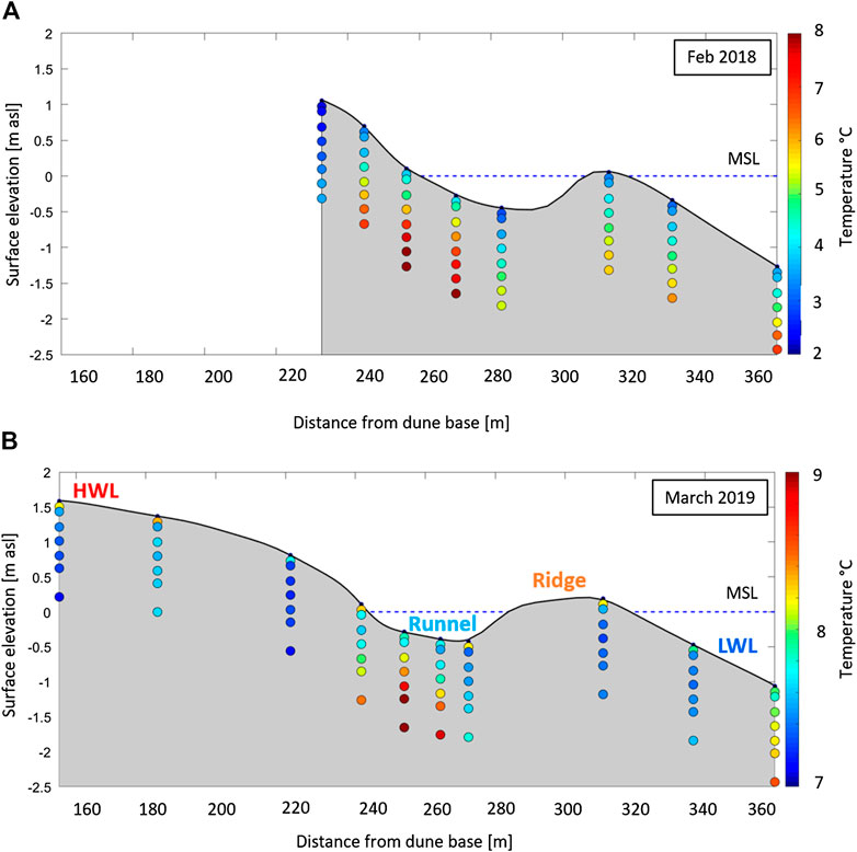
FIGURE 2. Measured temperature profiles for (A) February 2018 and (B) March 2019. Exfiltrating conditions are assumed to occur, where porewater’s temperatures are higher in ∼2 m depth compared to the top and decreases toward the surface. Infiltration conditions are assumed to occur, where temperature sensors show almost continuous temperature of seawater from top to 2 m depth.

Quantifying In- and Exfiltration Rates

Different techniques were used to determine the volumes of in- and exfiltrating water. In general, seepage meters and/or lysimeters were installed during spring tide, while ²²²Rn and temperature were measured simultaneously or within the ensuing week to ensure the mean LWL during low tide could be reached. To compare estimates of different methods, all measurements were reported in Darcy-velocities [m day⁻¹]. Assumptions made for up-scaling are described below for each method.

Handheld Lysimeter Construction and Sampling

Infiltration was measured using a modified pan lysimeter based on the work of Jordan (1968) and Heiss et al. (2014) above the permanently saturated beach areas within the intertidal zone up to the mean spring tide mark.The lysimeters were constructed using a PE-cylinder (Ø 110 mm, height: 500 mm), whose bottom closed conically toward a tube connection (FEP-tube 4 mm × 6 mm, Supplementary Figure S1A). This allowed a complete drainage of the buried lysimeters. The upper part of the cylinder was closed with a porous filter plate (PE, 200 μm, thickness = 5 mm), which was protected by a filter sleeve. The remaining space was filled up with sediment from the site (predominantly fine sand). Previous lab experiments by Heiss et al. (2014) revealed that this approach limits the preferential flow into the lysimeter. A second tube connection (4 mm × 6 mm) was attached directly below the porous plate to ensure atmospheric pressure inside the device in order to enable water infiltration.

In October 2016, March 2017, and August 2017, six lysimeters were buried in the unsaturated beach around the HWL at a depth of approximately 20 cm. To limit disturbance of the system, a hole was dug down to the groundwater level and the lysimeters were inserted horizontally into the undisturbed sediment, thereby maintaining an undisturbed sediment cover (Supplementary Figure S1B). Sediment gaps were carefully filled with sand before the hole was completely refilled. The lysimeters were left in the sand for 1 day (24 h) to adapt before they were regularly emptied after one tidal cycle using a peristaltic pump (Peristaltic Pump VDC 12 Standard, Eijkelkamp Soil & Water) connected to the tubing system. In order to prevent surface water from entering the drainage or venting tube during high water, both tubes were equipped with wooden swimmers and fixed on a wooden beam. Shallow piezometers (high-density polyethylene, Ø 63/51.4 mm) equipped with pressure loggers were installed close to the lysimeters in order to continuously measure the groundwater level. This way, misinterpretation as a result of unintentional inflow of groundwater into the lysimeters was prevented. Sand accumulations inside the piezometers were impeded by the usage of short filter screens (Ø 63/51.4 mm × 500 mm) with a slot width of 0.3 mm surrounded by a filter sleeve. The lysimeters provided volumes in m³ per tidal cycle per m² beach, which were doubled (semidiurnal tides) to determine a rate in m per day.

Seepage Meter Construction and Sampling

Seepage meters were constructed from PE-cylinders (150 mm height, Ø 670 mm) after Lee (1977) and were unilaterally closed with an unlockable tube port on top (12 mm, Supplementary Figure S2A). In October 2016 and August 2017, four seepage meters were carefully placed slightly inclined into the saturated sediment from the LWL to the HWL (protruding ∼5 cm from the sediment surface) (Supplementary Figure S2B). The locations of seepage meters were varied several times along the transect to reflect the entire intertidal zone. The port was left open for adapting to the environment for at least 30 min. Subsequently, a 3 L PE bag was attached to the outlet for a minimum of 30 min (up to several hours) without changing. Longer adaption or collecting times were not possible for the study site, because strong wave movement threatened to displace the seepage meters. Note that due to the short adaption times we suppose that the water collected in the bags was not pure SGD but seawater which was displaced by discharging groundwater. This means that further geochemical water analysis (e.g., for salinity) would not have been meaningful. Hence, we could not distinguish between fresh and saline SGD in the field using seepage meters. The bags were filled with 500 ml of seawater to impede underestimation of fluxes as mentioned in Shaw and Prepas (1989) and to enable infiltration from the seepage meter into the sediment (Michael et al., 2003). Volume loss or gain was determined after the respective sampling time for each seepage meter. Seepage meters only provided point measurements over a certain period of time and no information about the temporal development of the rates during a tidal cycle as they could not remain in the sediment for long. Additionally, it was not possible to recover them during high tide as they were submerged by ∼3 m water depth. To upscale to daily infiltration rates the measured rates (m³ per m² per hour) were assumed to be representative for the time period when the respective beach location was inundated. The inundation time for each sampling point was determined from surface water level and respective surface elevation. In order to calculate exfiltration rates, point measurements were assumed to be representative for the entire tidal cycle, regardless of rising or falling water levels. Measured rates were then extrapolated for 1 day.

Analysis of ²²²Rn in Pore Water

To analyze ²²²Rn, multiple discrete 1.5 L pore water samples were extracted in a range of 0.5–2.0 m depth below the surface during five field campaigns in March, May, August and September 2017 as well as in February 2018. Per campaign two to three pore water profiles were sampled. Each profile consisted of at least two and up to 4 samples (Supplementary Figure S3). The sampling sites covered the entire intertidal zone, but only samples taken in infiltration zones are discussed in this study. In exfiltration zones, where the groundwater discharging is relatively old, ²²²Rn cannot be applied as tracer due to its short half-life of 3.8 days and mixing of water masses of different origin. Fresh groundwater deriving from the freshwater lens is assumed to be in equilibrium with surrounding sediments or may deliver even higher loads of ²²²Rn released by lithologies other than beach sand. Samples were assumed to be a mixture of seawater and freshwater, when the salinity deviated by > 10% from seawater salinity and were subsequently excluded from rate calculations. Porewater was extracted using stainless steel push point samplers and a peristaltic pump (Peristaltic Pump VDC 12 Standard, Eijkelkamp Soil & Water) at low flow rates (<0.5 L/min) to avoid degassing. The polyethylene terephthalate (PET) sample bottle was purged by about one bottle volume and filled without headspace.

²²²Rn activities were measured in a closed air-loop setup, using a radon-in-air monitor (RAD 7 Radon Monitor, Durridge Company, Inc.; Supplementary Figure S4). Prior to measurement, about 7 ml of the sample were carefully discarded to create a headspace. Air was bubbled through the water sample using the internal pump of RAD7 and the stripped ²²²Rn was transferred in a closed air loop to the detection chamber. From March to September 2017, an active moisture exchanger was implemented in-line with the drying column. In February 2018, the air-loop setup was used without an active moisture exchanger. Counts were integrated from 5 to 8 cycles with each 10–15 min counting time. To convert RAD7 counts into radon-in-water concentrations air loop ²²²Rn-concentrations were multiplied by a conversion coefficient. This coefficient takes into account sample and air-loop volumes as well as temperature and salinity. The samples were corrected individually for the decay, which occurred between sampling and analysis. Yet, all samples were measured within 24 h after sampling.

Infiltration rates were deduced from the depth distribution of pore water residence times assuming 1D-vertical flow with the latter derived from measured ²²²Rn activities. Under the assumption that the half-life of the parent isotope ²²⁶Ra is much longer (1,602 years) than of ²²²Rn (3.8 days), the Bateman Equation (Bateman, 1910) can be simplified to describe the ingrowth of ²²²Rn in a closed system:

${}_{}{}^{222}Rn={}_{eq}{}^{222}Rn\left(1-e^{-{\lambda }_{222Rn}\tau }\right)(1)$

Here the pore water ²²²Rn activity is a function of the equilibrium activity ${}_{eq}{}^{222}Rn$, the specific decay constant ${\lambda }_{222Rn}=0.1813\left[d^{-1}\right]$and the residence time$\tau$.

Rearranged, the residence time can be calculated:

$\tau =\frac{1}{{\lambda }_{222Rn}} ln \left(1-\frac{{}_{}{}^{222}Rn}{{}_{eq}{}^{222}Rn}\right)(2)$

In this study, ${}_{eq}{}^{222}Rn$ was defined by the activity of a groundwater sample, that was retrieved from 2 m below surface in the runnel exfiltration zone in September 2018 (Supplementary Figure S3). According to modeling results from Beck et al. (2017) and Grünenbaum et al. (2020), pore water residence times at this location ranged between several months up to years and are, thus, sufficiently long to approximate${}_{eq}{}^{222}Rn$.

According to Tamborski et al. (2017), residence time calculations have reasonable uncertainties when residence times are longer than 0.5 days, but shorter than 7 days. The lower limit is based on radon detectability and background activities such as the seawater radon end-member, whereas the upper limit results from the asymptotical approach of ${}_{eq}{}^{222}Rn$ during ²²²Rn ingrowth.

Assuming the uniform distribution of the parent isotope ²²⁶Ra in the sediment and steady-state pore water velocities at seawater infiltration sites, the slope of the linear regression function of the ²²²Rn residence time vs. depth represents the fluid velocity, which was multiplied by the effective porosity ($n_e=0.3$) to obtain the Darcy flux.

Temperature Sensors

The quantitative use of temperature is based on solving the advection-conduction-dispersion equation for heat transport in porous media and relies on solutions (depending on boundary conditions) to the partial differential equation for heat transport (Anderson, 2005).

This can be written as (Anderson, 2005; Schmidt et al., 2006):

$\frac{{\text{k}}_{\text{e}}}{\text{ρc}}{\nabla }^2\text{T}-\frac{{\text{ρ}}_{\text{w}}{\text{c}}_{\text{w}}}{\text{ρc}}\nabla \cdot \left({\text{Tq}}_{\text{z}}\right)=\frac{\partial \text{T}}{\partial \text{t}}(3)$

Where T is temperature (°C), t is time (s), ρc is the volumetric heat capacity of the fluid-solid system (J m⁻³ K⁻¹) and is often written as ρc = nρ_wc_w + (1 − n) ρ_sc_s with ρ_wc_w (J m⁻³ K⁻¹) being the volumetric heat capacity of the liquid phase and ρ_sc_s (J m⁻³ K⁻¹) the volumetric heat capacity of the solid phase, q_z (m s⁻¹) is the Darcy seepage velocity, while k_e (J s⁻¹ m⁻¹ K⁻¹) is the effective thermal conductivity of the saturated sediment with no advective flow.

This equation can be solved analytically or numerically for 1D heat transport assuming 1D vertical flow for either steady state or non-steady state boundary conditions (Lapham, 1989; Rau et al., 2014; Munz and Schmidt, 2017). For steady state 1D heat transport and Dirichlet-Type boundary conditions at the upper and lower ends, the solution of Eq. 3 can be written as (Bredehoeft and Papaopulos, 1965):

$T\left(z\right)=\frac{\exp \left(z\frac{q_z{\rho }_w{c}_w}{k_e}\right)-1}{\exp \left(L\frac{q_z{\rho }_w{c}_w}{k_e}\right)-1}\times \left(T_L-T_0\right)+T_0(4)$

L is the depth (m) of the lower boundary condition (m), while T_L is the temperature (°C) at depth L and is usually assumed to be the regional groundwater temperature, T₀ is the temperature (°C) of the upper boundary condition, usually the surface water temperature or, as in our case, just below the sediment-water interface. As the name implies this solution assumes that there is no temporal change in either boundary condition or the groundwater flux and that sediment properties are constant and uniform in time and space.

Typically, the steady state model is fitted to a measured temperature profile by minimizing the root mean square error by varying the Darcy velocity, assuming all other parameters are known. Negative Darcy velocities indicate groundwater exfiltration while positive values are infiltration of seawater into the subsurface.

The BT-lances were made of pointed stainless steel tubing with a diameter of 1 cm and equipped with eight high sensitivity thermistors (5 kΩ NTC thermistor, 0.2% from Reichelt GMBH) (Supplementary Figure S5). The thermistors were attached to a stainless steel rod at intervals of 0.08, 0.15, 0.37, 0.57, 0.78, 0.96, 1.16, and 1.37 m that was inserted into the stainless steel housing. The free space was back-filled with fine quartz sand with a similar grain size to the field site. This was an attempt to replicate the thermal characteristics of the beach and to avoid convection that can occur within an air-filled or water-filled tube. Each sensor was attached to a circuit board that measured the resistance of the thermistors. Resistivity was converted to a digital value using an 18 bit ADC and stored to flash memory. Resistivity was converted to temperature values using the function supplied with the thermistors. The electronic setup was based on Arduino architecture and was developed as part of our push towards low-cost high-resolution measurement devices for environmental applications. Tests in the laboratory have shown that each sensor has a resolution of ∼0.003°C, and the difference between sensors was around 0.007°C. The high resolution can be attributed to the high-resolution ADC and high quality thermistors.

Temperature profiles were measured from the LWL towards the HWL in February 2018 and March 2019. We did not extend the temperature mapping to the HWL to avoid complications due to heat transport in the unsaturated sands. The temperature lance was driven into the sediment and then left to equilibrate (for ∼10 min). In total nine temperature profiles were made along the transect. The steady state model was fitted to each profile by varying the Darcy flux to minimize the Root-mean-square error (RMSE) between the model and the measurements as in Schmidt et al. (2006), see Supplementary Figure S6. The thermal parameters were largely taken from Rau et al. (2012), who conducted detailed heat transport experiments on saturated clean quartz sand in the laboratory. The thermal conductivity and volumetric heat capacity of saturated sand were 3.8 J s⁻¹ m⁻¹ K⁻¹ and 3.23 × 10⁶ J m⁻³ K⁻¹ respectively. Despite groundwater temperatures never being truly stationary, especially in small island aquifers, we have defined the lower boundary as the depth at which the yearly amplitude in temperature variations is less than 1°C. Based on an evaluation of nested bores located about 3 km to the east of the site (Holt et al., 2019) we set the lower boundary condition as the mean yearly temperature from bore DN-d at a value of 10.6 °C from a depth of 6.4 m. The standard deviation (1σ) in temperatures at this depth was 0.3°C.

Numerical Model

Grünenbaum et al. (2020) developed a two-dimensional cross-sectional model of the study site (from dune base 700 m toward the sea) in order to estimate the groundwater flow, residence times, and salinity distribution at the site, thereby using a time-averaged topography (Supplementary Figure S7). Several model cases were set up with the density-dependent groundwater flow model SEAWAT, in order to display the model’s sensitivity against changes in model parameters such as dispersivity, hydraulic conductivity, and the groundwater flux from the island’s freshwater lens. The existence and extension of a groundwater divide below the ridge was considered in the tide-averaged head calculation in different scenarios. The analysis of the water budget of one selected model provided approximated fluxes through the STE per day along 1 m of shoreline. The model chosen was considered the most realistic one based on shallow salinity measurements, the conceptual model proposed by Waska et al. (2019), and hydraulic parameters by Beck et al. (2017). Note that the influence of waves was not considered in the presented modeling approach. Further model assumptions were the use of tide average heads neglecting storm flood events or spring/neap tides, the estimation of fresh groundwater flux, as well as the uncertainty of the calibration parameters. SGD fluxes can be assumed to be between 0.5 to 2 times the provided rates as also stated in Beck et al. (2017). This estimation is based on findings from Xin et al. (2010), who compared tide-resolved modeling approaches without and with wave setup. The latter resulted in an increase of 33% in the total SGD rates plus a doubled saline SGD rate through the USP.

Morphodynamic Changes and Upscaling

The change in beach topography was measured with a 3D Laser scanner (FARO Focus 3D X 130) in several campaigns (March 2017, May 2017, August 2017, and February 2018). A point distance of 3.068 mm per 10 m was used, recommended for outdoor scans with a distance between the scanner and the object of interest greater than 20 m. In total, eight scans per sampling campaign were conducted and combined, in order to completely cover the study site (200 m × 200 m). Post-processing was done with the FARO software Scene 5.4. The accuracy was strongly dependent on environmental conditions during scanning in the field, but was always under 10 cm.

The measured and modeled in- and exfiltration rates (Darcy-velocities obtained with the various methods) were correlated to the respective topographic heights. Using the areal topography from the 3D laser scans, these rates were transformed to volumetric fluxes for the whole study area. The scanning results were subsequently assigned to the respective in- or exfiltration zone (HWL, Runnel, Ridge, LWL) for the individual campaigns based on relative position in the intertidal zone (Figure 5; Supplementary Figure 8) and findings from Figure 3. The resulting volumetric in- and exfiltration rates between mean HWL (1.37 m Above Sea Level) and mean LWL (−1.37 m ASL) were normalized to 1 m shoreline.

FIGURE 3

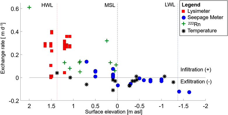
FIGURE 3. Measured exchange rates plotted vs. surface elevation. Positive rates indicate infiltration and negative rates exfiltration. The different techniques are illustrated with red squares (lysimeters), blue circles (seepage meters), green crosses (²²²Rn), and black stars (temperature sensors). Mean HWL (red), MSL (black), and mean LWL (blue) are shown as dashed lines.

Results and Discussion

Spatial Variability of Exchange Rates

Temperature profiles can be used to qualitatively identify in- or exfiltration zones. As sampling was done in winter, warmer water near the surface should indicate discharge areas. Such upwelling of warm groundwater was observed in the runnel and at the LWL. In contrast, very low SGD rates or infiltrating conditions are indicated by little increase of temperature with depth. This was observed at the ridge and at the HWL (Figure 2). These effects were particularly pronounced in February 2018 due to the higher temperature difference between ground and surface water compared to March 2019. Hence, the temperature profiles allow to rapidly screen a field site for potential SGD areas and relate this to the site morphology in a runnel-ridge system (Figure 2B).

Groundwater exchange rates were estimated based on seepage meters, lysimeters, ²²²Rn measurements, and heat modeling of the temperature sensors (Supplementary Table S1). Note that the subsequent discussion of measured exchange rates is limited to their spatial variability at the beach as the techniques were used over different seasons, under varying environmental conditions, at various locations, and not all simultaneously. As such the present data, though extensive, is not sufficient to clearly attribute exchange rates to factors of influence such as seasonality reflected by tidal variation or a change in the terrestrial groundwater flow.

Infiltration rates at the site were found to span over two orders of magnitude and ranged between 0.001 and 0.61 m day⁻¹. Measured exfiltration rates were mostly lower and were also less variable, fluctuating between −0.007 and −0.13 m day⁻¹. Similar SGD rates were determined, for example, at Waquoit Bay (∼0.05–0.3 m day⁻¹) based on radon and radium time series in bay waters and seepage meters measurements from 2002 to 2003 (Mulligan and Charette, 2006).

The water exchange rates plotted vs. surface elevation using all methods and measurements showed that net infiltration predominantly occurred above MSL, while net exfiltration prevailed below MSL (Figure 3). The high fluctuations of infiltration rates in temporally unsaturated beach areas (≥1 m ASL) were likely caused by a spatial variability in the position of the HWL. Thereby, smaller infiltration rates might be attributed to single swash events instead of constant infiltration of seawater over a certain period. In contrast to the partly unsaturated HWL zone, infiltration rates in saturated beach areas (∼<1 m ASL) were mostly lower (≤0.1 m day⁻¹).

Figure 4 shows how the rates varied along the cross-section visualizing the different in- and exfiltration zones (HWL, Runnel, Ridge, LWL, compare Figure 2A). Infiltration rates at the HWL were found to fluctuate the most, i.e., covering rates from 0.001 to 0.61 m day⁻¹, while infiltration rates at the ridge were mostly lower and varied between 0.03 and 0.11 m day⁻¹. Predominately exfiltrating conditions were encountered in the runnel and at the LWL spanning rates between −0.007 and −0.06 m day⁻¹ (runnel) and −0.02 and −0.13 m day⁻¹ (LWL). Compared to measured exchange rates, numerical modeling by Grünenbaum et al. (2020) displayed the same spatial distribution of in- and exfiltration zones, but infiltration rates at the HWL were generally lower (∼0.1 m day⁻¹). Note that only one model run with averaged beach topography was used for flux calculation.

FIGURE 4

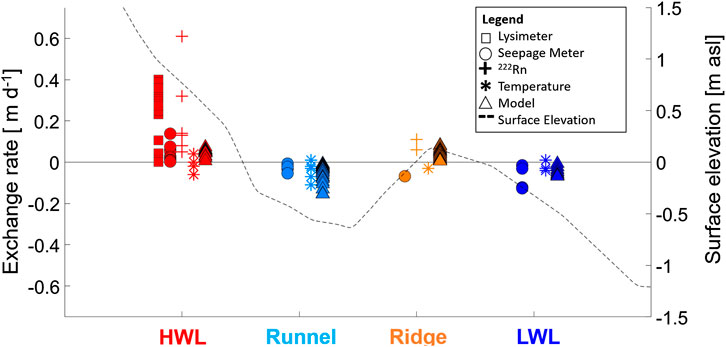
FIGURE 4. Comparison of all measured exchange rates across respective in- or exfiltration zones (HWL = red, Runnel = light blue, Ridge = orange, LWL = blue). The different methods are indicated with squares (lysimeters), circles (seepage meters), crosses (²²²Rn), and stars (temperature sensors). Model results are also included (triangles). The exemplary surface elevation from October 2016 is added to visualize the principal zone distribution along the cross-section.

In order to visualize the topography changes and the spatial distribution of in- and exfiltration zones, representative selected LIDAR scan results of two seasons (August 2017 and February 2018) are shown in Figure 5. Whereas the runnel-ridge system was always present, the location and extension of both runnel and ridge differed significantly for the two seasons. In August 2017, two separate ridges existed, a long-shore ridge and a ridge-like feature striking in 45° from the HWL towards the LWL. Conversely, the beach topography in February 2018 showed a typical long-shore runnel-ridge sequence from the HWL towards the sea. Corresponding exchange rates plotted into the scans mostly showed infiltrating conditions at the HWL and the ridge and exfiltrating conditions at the LWL and the runnel. Deviations were occasionally observed, e.g., in February 2018 at the LWL and in the HWL zone. Based on the temperature distribution in Figure 2, it appears that the fact that exfiltration rates were calculated above MSL from temperature data is possibly the result of the assumption of 1D flow, while in reality it is 2-(or 3) dimensional.

FIGURE 5

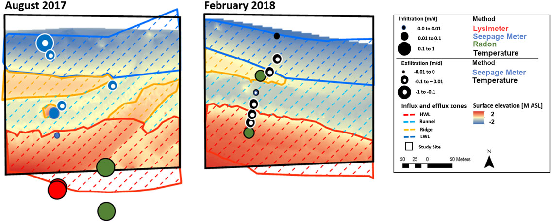
FIGURE 5. Determination of beach topography (∼200 m × ∼200 m, black box) for August 2017 and February 2018 including both location and extent of measured exchange rates. Infiltration rates based on lysimeters measurements (red circles) were displayed as mean value from all measurements for respective sampling campaign at same location. Dashed polygons indicate topography-based classification of in- and exfiltration zones (HWL, Runnel, Ridge, LWL) for the study site based on results from Figure 3 suggesting net infiltration above MSL and net exfiltration below MSL. Zones for HWL and LWL were linearly extended or reduced beyond the boundaries of the study site (black box) to cover the entire area between mean high water (+1.37 m ASL) and mean low water (−1.37 m ASL). Infiltration rates outside the black box were partially measured due to a shift in HWL during sampling.

In order to extrapolate the point measurements to the entire study area mapped by the scans, the respective zones (HWL, Runnel, Ridge, LWL) were allocated in all topography scans (Figure 5, Supplementary Figure S8). This was done based on results from Figure 3 suggesting net infiltration above MSL and net exfiltration below MSL. Zones for HWL and LWL were linearly extended or reduced to cover the entire area between mean high water (+1.37 m ASL) and mean low water (−1.37 m ASL).

Spatial Extrapolation of Exchange Rates

Figure 6A shows the areal size in m² normalized to 1 m shoreline of the respective in- and exfiltration zones based on all scan results (Supplementary Figure 8), in the following referred to as “zone length” in m.

FIGURE 6

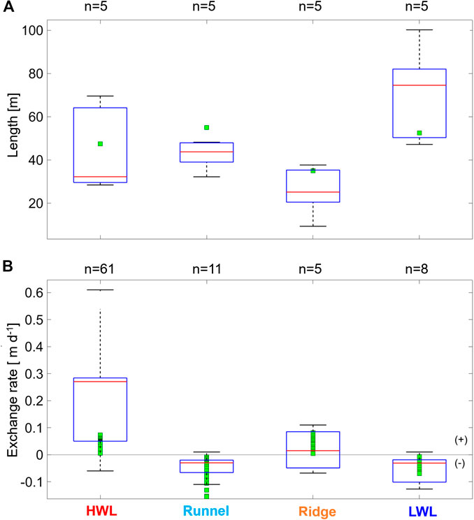
FIGURE 6. (A) Areal variation of respective in- and exfiltration zone (HWL, Runnel, Ridge, LWL) in the intertidal zone normalized to 1 m shoreline for sampling campaigns March (1) 2017, March (2) 2017, May 2017, August 2017, and February 2018 based on Supplementary Figure S8. Green squares indicate model results. (B) Variation of measured exchange rates within respective in- and exfiltration zone (HWL, Runnel, Ridge, LWL) in the intertidal zone. Positive rates indicate infiltration, negative rates exfiltration, respectively. Green squares indicate model results. Black dots are values that are more than 1.5 times the interquartile range away from the top or bottom of the box. Red line indicates median of boxplot. Number of statistics (n) is given above.

Whereas the zone length of HWL and LWL varied between ∼30 and ∼70 m, and ∼50 and ∼95 m respectively, the size of the runnel and ridge zones fluctuated between 35 and 50 m, and 15 and 40 m, respectively (Figure 6A).

Subsequently, the areal size was multiplied with all the rates measured (Figure 6B) to get an idea on the volumes of in- and exfiltrating water along 1 m of shoreline for each in- or exfiltration zone. Note that the number of measurements is significantly different for each zone.

Figure 7 shows that the variation of water volumes circulating through the intertidal zone was relatively high. Especially at the HWL, the total infiltration fluxes ranged between almost zero and 35 m³ per day and m shoreline. Most of the rates were measured at the HWL, i.e., not equally distributed over the entire infiltration zone. Single point measurements below the HWL suggested the infiltration rates to decrease toward topographical lower laying beach areas (Figure 3). Thus, it is possible that the extrapolation of point measurements to the entire zone leads to an overestimation of inflow. The total infiltration into the ridge is indicated to be generally lower compared to the HWL, with a total infiltration of maximum 20 m³ per day and m shoreline. Total exfiltration within the intertidal zone consists of up to −1.9 m³ per day and m shoreline into the runnel and −13 m³ per day and m shoreline at the LWL.

FIGURE 7

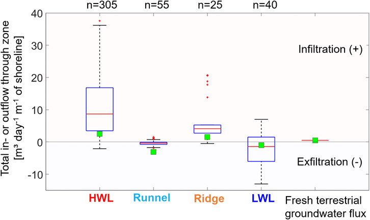
FIGURE 7. Total in- and outflow within the in- and exfiltration zones at the northern beach of Spiekeroog (intertidal zone) for 1m shoreline. For total water budgeting, fresh groundwater flux (estimated with 0.75 m³ per day and meter of shoreline from Beck et al. (2017)) has to be considered as additional proportion infiltration. Green squares indicate results from models water budget (Grünenbaum et al., 2020). Red dots are values that are more than 1.5 times the interquartile range away from the top or bottom of the box. Red line indicates median of boxplot. Number of statistics (n) is given above.

These results suggest that total infiltration (∼12 m³ per day and m shoreline) exceeds total exfiltration (∼4.5 m³ per day and m shoreline). This is the case for both field measurements and the numerical simulation (In: 6 m³ per day and m shoreline/Out: −5.5 m³ per day and m shoreline), with modeling limited to the intertidal zone. During field work, the terrestrial groundwater flux was not determined as an inflow component. If it is considered as an additional inflow proportion of approximately 0.75 m³ per day and m shoreline (Beck et al., 2017) as partially done in the simulations from Grünenbaum et al. (2020), the discrepancy between total in- and outflow is even larger. One explanation could be possible overestimation of total infiltration in the infiltration zone around the HWL, as discussed above. Another reason for the difference could be that the subtidal area below the LWL was neither investigated by flux measurements in the field nor considered within areal extrapolation, while model results suggest that a proportion of the water discharges below the LWL (Grünenbaum et al., 2020).

To assess the relevance of SGD on a larger scale, water fluxes determined at the northern beach of Spiekeroog were assumed to be representative for the beaches of all barrier islands, which are facing the open North Sea and are connected to a freshwater lens. Measured rates were extrapolated to the entire East Frisian barrier island chain from Borkum to Wangerooge (∼56 km) based on previous estimations from Beck et al. (2017). In comparison to medium runoff from the rivers Weser, Elbe and Ems into the German Bright, which is about 1,200 m³ per second (Becker et al., 1999), the SGD proportion (fresh and salty) from the East Frisian barrier island chain is up to 0.8% of the riverine discharge. The median SGD proportion is even lower (0.2%) and matches water budget calculations (0.3%) based on the numerical simulation from Grünenbaum et al. (2020).

Method Applicability and Limitations at a High Energy Beach

In general, the exchange rates measured by the different techniques at the study site agreed reasonably well. Problems arise from the temporal variations of rates over a tidal cycle, up-scaling, the sampling dates that were not consistent between methods and especially the high-energy setting itself. The latter aggravates the use of commonly applied methods, e.g., seepage meter measurements over longer time scales and requires assumptions regarding the rates’ temporal development.

Direct Measurements

Lysimeters

The results suggest that the use of lysimeters to determine unsaturated infiltration in high-energy settings for a limited timeframe is suitable. In sufficiently thick unsaturated beach zones, they are easy to install and (after a reasonable adaption time of ∼1 day) resistant to the wave dynamics that periodically occur at the sampling site. The lysimeters were able to cover a range of infiltration rates between 0.001 and almost 0.6 m day⁻¹, whereas replica measurements at the same location provided reliable results (Mean Absolute Deviation of ∼0.005 m day⁻¹). In order to resolve the temporal development during a tidal cycle, the lysimeters should be equipped with pressure transducers as done in Heiss et al. (2014) in future studies. Difficulties arise from the continuous sediment relocation at high energy beaches resulting in an uncontrolled shrinkage or growth of the unsaturated zone within days to weeks and burial of equipment. This means that long-term measurements of unsaturated infiltration are impeded at high energy beaches.

Seepage Meters

Seepage meters provided overall comparable (saturated) infiltration and exfiltration rates from HWL to LWL between replica measurements. Nevertheless, applicability in the field was difficult due to weather and wind conditions. Indeed, seepage meter measurements could not be conducted during all campaigns, because the attached plastic bags were influenced by stronger wave activity, which was reported in previous studies (e.g., Libelo and MacIntyre, 1994; Burnett et al., 2006). Wave activity and resulting equipment loss prevent longer adaptation times to the field site. As a result, only measurements over short times (hours) could be conducted, which does likely not lead to unrealistic fluxes, but inhibits further chemical investigations of the collected (exfiltrating) water, e.g., to determine the salinity, because the water under the seepage meter is not completely exchanged yet. For the study site, automatic seepage meters equipped with flow meters, as done in terrestrial studies (e.g., Krupa et al., 1998), would be more appropriate in order to collect long-term information over several tidal cycle. To stabilize the position of seepage meter and protect it for flipping in the waves, it should be additionally weighted down.

Indirect Measurements

At the study site, the flow field in the intertidal zone appears to be rather complicated considering the effect of tidal pumping, a strong wave-set up, and a changing beach topography (Waska et al., 2019 or Supplementary Figure S8). Indirect methods using radon residence times and temperature profiles complement direct volumetric methods but rely on a set of assumptions (e. g., steady state, respective flow conditions). Assumptions and related problems are discussed below.

²²²Rn in Pore Waters

The infiltration rates obtained by the ²²²Rn tracer approach are in good agreement to those of lysimeters, temperature sensors, and seepage meters. Most radon derived infiltration rates were lower than respective lysimeter infiltration rates and higher than those derived from temperature sensors or seepage meters (Figure 3).

Infiltration rates were obtained by fitting a linear regression function to pore water residence times derived from distinct ²²²Rn pore water measurements. Sediment inhomogeneity, i.e. a non-uniform distribution of sediment-bound ²²⁶Ra or varying grain sizes and mixing of water masses of different ages or salinity will affect the ²²²Rn distribution within the sediment and have been identified as major constraints for the applicability of this method (Tamborski et al., 2017). Furthermore, ²²⁶Ra accumulation is likely regulated by the presence of manganese (hydr)oxides (Dulaiova et al., 2008). Therefore, active manganese cycling within the sediment body may cause a non-uniform distribution of sediment bound ²²⁶Ra. Beck et al. (2017) reported rather small variations in grain size for the Spiekeroog study site, with however some carbonate shell layers affecting sediment permeability, porosity, and pore water flow conditions. Generally, as sediment bound ²²⁶Ra is the source of pore water radon, smaller grain sizes would lead to a higher specific surface and finally to a higher radon emanation to pore waters. Nonetheless, beach sediments from Spiekeroog Island are redistributed by erosion and sedimentation, e.g., on seasonal timescales (Flemming and Davis, 1994; Waska et al., 2019). Thus, pronounced redox-driven Mn oxide enrichments are unlikely and the overall effect of sediment inhomogeneity on calculated residence times and infiltration rates is suggested to be rather small for Spiekeroog sediments. Additionally, the pore water receives an integrated ²²²Rn signal of the sediment through which it has traveled. This may further compensate small scale sediment heterogeneities. Radon evasion across the saturated-unsaturated sediment interface, as reported by Colbert et al. (2008), might be of minor importance for the rate calculations at Spiekeroog because ²²²Rn samples extracted from the temporally unsaturated part of the sediment do not show a significant radon deficit compared to samples from permanently saturated sediments.

In general, the restriction to a small ingrowth period of 0.5–7 days (Tamborski et al., 2017) limits the applicability of this method to zones of seawater infiltration (HWL, Ridge) at the Spiekeroog study site. If background activities in seawater are low, the lower restriction derives from detection limits of ²²²Rn. This limit may be lowered by increasing the analytical sensitivity, for example by increasing sample volumes, detector size or reducing air volumes. However, the upper limit derives from the theoretical temporal evolution of ²²²Rn (Eq. 1), which asymptotically approaches the equilibrium activity ${}_{eq}{}^{222}Rn$. As a consequence, model uncertainties are amplified, when ²²²Rn activities are close to ${}_{eq}{}^{222}Rn$, producing large errors in residence times (Supplementary Figure S3).

In this study, the equilibrium activity ${}_{eq}{}^{222}Rn$ was approximated by sampling deep pore water from a representative exfiltration site. This is in contrast to other studies, which determined the equilibrium activity experimentally (Goodridge and Melack, 2014; Colbert et al., 2008; Tamborski et al., 2017). This approach was chosen as the hydrogeological setting is well known (Beck et al., 2017; Grünenbaum et al., 2020) and experimental approaches are often influenced by artefacts as they require an accurate imitation of natural conditions in the laboratory. However, a limitation of our method is that the equilibrium activity ${}_{eq}{}^{222}Rn$ was only determined once and not for each sampling event separately, although intertidal pore water temperatures are highly variable throughout the year (Waska et al., 2019). ${}_{eq}{}^{222}Rn$ was determined based on analyses in September (summer), when pore waters were comparably warm. However, we are not able to assess any seasonal effects based on our dataset.

Temperature Sensors (1D-Heat Transport Solution)

The use of temperature as a tracer in the coastal zone is limited, but it offers a useful addition to other tracer methods as it can quantify infiltration and exfiltration in saturated sediments, is cheap to measure directly in the field, and is ubiquitous in natural systems. Taniguchi et al. (2003) used temperature profiles to estimate vertical groundwater fluxes in the Cockburn sound (Australia) using the 1D steady state and non-steady state models while Tirado-Conde et al. (2019) recently compared exchange fluxes using the steady state temperature model and direct seepage meter measurements at a calm lagoon of the North Sea coast in Denmark. In the later study fluxes based on temperature measurements better matched seepage meter values in areas with a higher proportion of freshwater discharge than in areas dominated by recirculating seawater. This was explained by the complexity of the flow field in zones of circulating seawater, which is not limited to one dimension. The temperature profiles from the site studied here (Figure 2) show that temperature sensors can clearly delineate upwelling warm groundwater during winter in the runnel and LWL as well as locations with either low SGD flux or infiltrating conditions. This qualitative pattern in temperature profiles can be used as an additional tool to rapidly screen a field site for potential SGD and submarine groundwater recharge areas and relate this to the site morphology. This could assist in an optimized sampling strategy for detailed and time-consuming method such as seepage meters. This SGD mapping approach becomes especially important for highly dynamic environments, where the sampling at the LWL is often difficult and prior planning is required. As previous studies have suggested already (Röper et al., 2014; Tirado-Conde et al., 2019), a large difference between seawater temperature and exfiltrating groundwater is necessary in order to distinguish between the different endmembers and set realistic boundary conditions. This generally occurs either in summer- or wintertime. Winter is preferred due to the low to moderate diurnal oscillations in sea water temperature, which makes the use of steady-state models more applicable. While the SGD fluxes calculated using the temperature lances are similar to the other methods, more work is needed to better understand how the assumptions of 1D heat transport and steady-state conditions influence the results. These are clearly a strong simplification, as flow and transport at such a highly dynamic beach site is in reality both transient and 3-dimensional. Despite this temperature offers a currently underutilized tracer in the coastal zone and with further refinement is likely to assist in quantifying SGD rates in the future (Kurylyk and Irvine 2019).

Conclusion and Outlook

This study provides insights into the spatial variability of exchange rates within a STE in a meso-tidal, highly dynamic environment. It is one of a few studies that presents a multiple-method approach with direct (lysimeter, seepage meter) and indirect measurements (radon and temperature as tracer) as well as a numerical model in order to determine in- and exfiltration rates across all seasons to give a general idea about the range of fluxes occurring at a high energy beach.

The results suggest the existence of two exfiltration areas (Runnel, LWL) and two infiltration areas (HWL, Ridge) in the intertidal zone of the respective northern beach of Spiekeroog Island, which were induced by beach topography. Predominantly infiltrating conditions were found above MSL and mostly exfiltrating conditions below MSL. Infiltration rates at the HWL covered the highest range and varied between 0.001 and 0.61 m day⁻¹. Exfiltration rates generally fluctuated around −0.1 m day¹. The exchange rates measured by different methods were over all comparable. This was a promising finding as some of the techniques have rarely been applied in coastal aquifers or were found to be error-prone in dynamic environments.

An analysis of spatially and temporally highly resolved exchange rates at a high-energy beach has so far not been conducted and is certainly challenging. Yet, flow and transport patterns can be expected to be highly transient, as are likely the in- and exfiltration rates. To conduct continuous measurements would hence be a valuable yet elaborate task for future investigations.

Topographic information in combination with measured exchange rates showed a significant movement of influx and efflux zones within the intertidal zone over time. Thereby, not only the location but also the extensions of the zones varied, which in turn influenced the up-scaling of total in- or outflow. Extrapolated total SGD fluxes into the southern North Sea from the East Frisian barrier island chain contribute to terrestrial runoff with less than 1%.

Data Availability Statement

The original contributions presented in the study are included in the article/Supplementary Material, further inquiries can be directed to the corresponding author.

Author Contributions

Planning of field work was carried out by all authors. JG, GM, and I carried out lysimeter and seepage meter measurements at the northern beach of Spiekeroog in October 2016, March and August 2017. JA, MB, and MK were responsible for analysis of ²²²Radon in pore water from March, May, August, September 2017, and February 2018. BG conducted temperature measurements in February 2018 and March 2019. I conducted the modeling work myself in a previous study, with the support of JG. Data interpretation, as well as manuscript and figure preparation were performed in joint discussion with all co-authors.

Funding

We want to thank the Lower Saxony Ministry of Science and Culture for funding the study as part of the BIME project (“Assessment of ground- and porewater-derived nutrient fluxes into the German North Sea – Is there a „Barrier Island Mass Effect?”, VW ZN 3184 MWK).

Conflict of Interest

The authors declare that the research was conducted in the absence of any commercial or financial relationships that could be construed as a potential conflict of interest.

The reviewer (JJT) declared a past co-authorship with several of the authors (JA and MB) to the handling editor.

Acknowledgments

We thank the Nationalparkverwaltung Niedersächsisches Wattenmeer (NLPV), in particular G. Scheiffart and C. Schulz, for permitting investigations at the northern beach site of Spiekeroog, as well as for the aerial image of the island. Many thanks to the Niedersächsicher Landesbetrieb für Wasserwirtschaft-, Küsten-und Naturschutz (NLWKN), especially J. Ihnken and his colleages, as well as H. Nicolai, G. Behrens and K. Schwalfenberg from the Institute for Chemistry and Biology of the Marine Environment (ICBM) in Wilhelmshaven, for their help during the campaigns planning progress and equipment transport. We thank the local community and employees of the researcher house Wittbülten. The students, L. Diehl, A. Harms, C.H. Lünsdorf, J. Otten, and J. Schulz are thanked for assistance during sampling. Many thanks to the Wasser-und Schifffahrtsverwaltung des Bundes (WSV) and the Bundesamt für Seeschifffahrt und Hydrographie (BSH) for providing data of the tide gauges. Finally, we want to thank the Ministry for Science and Art (lower Saxony) for funding the study as part of the BIME project (“Assessment of ground- and porewater-derived nutrient fluxes into the German North Sea – Is there a Barrier Island Mass Effect?”) and the participating colleges from the ICBM in Oldenburg/Wilhelmshaven and the Max-Planck Institute (MPI) in Bremen. BG is especially grateful for H. Waska funding and organizing his participation in the SGD experiments on Spiekeroog as part of the BIME project.

Supplementary Material

The Supplementary Material for this article can be found online at: https://www.frontiersin.org/articles/10.3389/feart.2020.571310/full#supplementary-material.

References

Abarca, E., Karam, H., Hemond, H. F., and Harvey, C. F. (2013). Transient groundwater dynamics in a coastal aquifer: the effects of tides, the lunar cycle, and the beach profile. Water Resour. Res. 49 (5), 2473–2488. doi:10.1002/wrcr.20075

CrossRef Full Text | Google Scholar

Anderson, M. P. (2005). Heat as a ground water tracer. Groundwater 43 (6), 951–968. doi:10.1111/j.1745-6584.2005.00052.x

CrossRef Full Text | Google Scholar

Anschutz, P., Smith, T., Mouret, A., Deborde, J., Bujan, S., Poirier, D., et al. (2009). Tidal sands as biogeochemical reactors. Estuar. Coast Shelf Sci. 84 (1), 84–90. doi:10.1016/j.ecss.2009.06.015

CrossRef Full Text | Google Scholar

Bateman, Η. (1910). Solution of a system of differential equations occurring in the theory of radioactive 815 transformations. Proc. Cambridge Phil. Soc. 15, 423–427.

CrossRef Full Text | Google Scholar

Beck, M., Reckhardt, A., Amelsberg, J., Bartholomä, A., Brumsack, H.-J., Cypionka, H., et al. (2017). The drivers of biogeochemistry in beach ecosystems: a cross-shore transect from the dunes to the low-water line. Mar. Chem. 190, 35–50. doi:10.1016/j.marchem.2017.01.001

CrossRef Full Text | Google Scholar

Becker, G., Giese, H., Isert, K., König, P., Langenberg, H., Pohlmann, T., et al. (1999). Mesoscale structures, fluxes and water mass variability in the German Bight as exemplified in the KUSTOS-experiments and numerical models. Dtsch. Hydrografische Z. 51 (2–3), 155–179. doi:10.1007/BF02764173

CrossRef Full Text | Google Scholar

Befus, K. M., Cardenas, M. B., Erler, D. V., Santos, I. R., and Eyre, B. D. (2013). Heat transport dynamics at a sandy intertidal zone. Water Resour. Res. 49, 3770–3786. doi:10.1002/wrcr.20325

CrossRef Full Text | Google Scholar

Blume, T., Krause, S., Meinikmann, K., and Lewandowski, J. (2013). Upscaling lacustrine groundwater discharge rates by fiber-optic distributed temperature sensing. Water Resour. Res. 49, 7929–7944. doi:10.1002/2012WR013215

CrossRef Full Text | Google Scholar

Bredehoeft, J. D., and Papaopulos, I. S. (1965). Rates of vertical groundwater movement estimated from the Earth’s thermal profile. Water Resour. Res. 1 (2), 325–328. doi:10.1029/WR1001i1002p00325

CrossRef Full Text | Google Scholar

Burnett, W., Aggarwal, P., Aureli, A., Bokuniewicz, H., Cable, J., Charette, M., et al. (2006). Quantifying submarine groundwater discharge in the coastal zone via multiple methods. Sci. Total Environ. 367 (2–3), 498–543. doi:10.1016/j.scitotenv.2006.05.009

PubMed Abstract | CrossRef Full Text | Google Scholar

Burnett, W. C., and Dulaiova, H. (2003). Estimating the dynamics of groundwater input into the coastal zone via continuous radon-222 measurements. J. Environ. 69 (1–2), 21–35. doi:10.1016/S0265-931X(03)00084-5

CrossRef Full Text

Burnett, W. C., Dulaiova, H., Huettel, M., Moore, W.S., and Taniguchi, M. (2003). Groundwater and pore water inputs to the coastal zone. Biogeochemistry 66 (1–2), 3–33. doi:10.1023/B:BIOG.0000006066.21240.53

CrossRef Full Text

Cable, J. E., Martin, J. B., and Jaeger, J. (2006). Exonerating Bernoulli? On evaluating the physical and biological processes affecting marine seepage meter measurements. Limnol. Oceanogr. Methods 4 (6), 172–183. doi:10.4319/lom.2006.4.172

CrossRef Full Text | Google Scholar

Cho, H.-M., Kim, G., Kwon, E. Y., Moosdorf, N., Garcia-Orellana, J., and Santos, I. R. (2018). Radium tracing nutrient inputs through submarine groundwater discharge in the global ocean. Sci. Rep. 8 (1), 2439. doi:10.1038/s41598-018-20806-2

CrossRef Full Text | Google Scholar

Colbert, S., Berelson, W., and Hammond, D. (2008). Radon‐222 budget in Catalina Harbor, California: 2. Flow dynamics and residence time in a tidal beach. Limnol. Oceanogr. 53 (2), 659–665. doi:10.4319/lo.2008.53.2.0659

PubMed Abstract | CrossRef Full Text | Google Scholar

Constantz, J. (2008). Heat as a tracer to determine streambed water exchanges. Water Resour. Res. 44, W00D10. doi:10.1029/2008WR006996

CrossRef Full Text | Google Scholar

Dobrynin, M., Gayer, G., Pleskachevsky, A., and Günther, H. (2010). Effect of waves and currents on the dynamics and seasonal variations of suspended particulate matter in the North Sea. J. Mar. Syst. 82 (1), 1–20. doi:10.1016/j.jmarsys.2010.02.012

CrossRef Full Text | Google Scholar

Dulaiova, H., Gonneea, M. E., Henderson, P. B., and Charette, M. A. (2008). Geochemical and physical sources of radon variation in a subterranean estuary—implications for groundwater radon activities in submarine groundwater discharge studies. Mar. Chem. 110 (1–2), 120–127. doi:10.1016/j.marchem.2008.02.011

CrossRef Full Text | Google Scholar

Evans, T. B., and Wilson, A. M. (2016). Groundwater transport and the freshwater–saltwater interface below sandy beaches. J. Hydrol. 538, 563–573. doi:10.1016/j.jhydrol.2016.04.014

CrossRef Full Text | Google Scholar

Flemming, B. W., and Davis, R. (1994). Holocene evolution, morphodynamics and sedimentology of the Spiekeroog barrier island system (southern North Sea). Senckenbergiana maritima. Frankfurt/Main 24 (1), 117–155.

CrossRef Full Text | Google Scholar

Giblin, A. E., and Gaines, A. G. (1990). Nitrogen inputs to a marine embayment: the importance of groundwater. Biogeochemistry 10 (3), 309–328. doi:10.1007/BF00003150

CrossRef Full Text | Google Scholar

Gilfedder, B., Peiffer, S., Poeschke, F., and Spirkaneder, A. (2018). Mapping and quantifying groundwater discharge to Lake Steißling and its influence on lake water chemistry. Grundwasser 23, 155–165. doi:10.1007/s00767-017-0386-8

CrossRef Full Text | Google Scholar

Goodridge, B. M., and Melack, J. M. (2014). Temporal evolution and variability of dissolved inorganic nitrogen in beach pore water revealed using radon residence times. Environ. Sci. Technol. 48 (24), 14211–14218. doi:10.1021/es504017j

CrossRef Full Text | Google Scholar

Greskowiak, J. (2014). Tide-induced salt-fingering flow during submarine groundwater discharge. Geophys. Res. Lett. 41, 6413–6419. doi:10.1002/2014GL061184

PubMed Abstract | CrossRef Full Text | Google Scholar

Grünenbaum, N., Greskowiak, J., Sültenfuß, J., and Massmann, G. (2020). Groundwater flow and residence times below a meso-tidal high-energy beach: a model-based analyses of salinity patterns and 3H-3He groundwater ages. J. Hydrol. 58, 124948. doi:10.1016/j.jhydrol.2020.124948

CrossRef Full Text | Google Scholar

Heiss, J. W., Post, V. E., Laattoe, T., Russoniello, C. J., and Michael, H. A. (2017). Physical controls on biogeochemical processes in intertidal zones of beach aquifers. Water Resour. Res. 53 (11), 9225–9244. doi:10.1002/2017WR021110

CrossRef Full Text | Google Scholar

Heiss, J. W., Ullman, W. J., and Michael, H. A. (2014). Swash zone moisture dynamics and unsaturated infiltration in two sandy beach aquifers. Estuar. Coast Shelf Sci. 143, 20–31. doi:10.1016/j.ecss.2014.03.015

CrossRef Full Text | Google Scholar

Holt, T., Greskowiak, J., Seibert, S., and Massmann, G. (2019). Modeling the evolution of a freshwater lens under highly dynamic conditions on a currently developing barrier island. Geofluids 2019, 9484657. doi:10.1155/2019/9484657

CrossRef Full Text | Google Scholar

Hwang, D. W., Lee, Y. W., and Kim, G. (2005). Large submarine groundwater discharge and benthic eutrophication in Bangdu Bay on volcanic Jeju Island, Korea. Limnol. Oceanogr. 50 (5), 1393–1403. doi:10.4319/lo.2005.50.5.1393

CrossRef Full Text | Google Scholar

Johannes, R. (1980). Ecological significance of the submarine discharge of groundwater. Marine Ecol.- Prog. Ser. 3 (4), 365–373. doi:10.3354/meps003365

CrossRef Full Text | Google Scholar

Jordan, C. F. (1968). A simple, tension-free lysimeter. Soil Sci. 105 (2), 81–86. doi:10.1097/00010694-196802000-00003

CrossRef Full Text | Google Scholar

King, C., and Williams, W. (1949). The formation and movement of sand bars by wave action. Geogr. J. 113, 70–85. doi:10.2307/1788907

CrossRef Full Text | Google Scholar

Krupa, S. L., Belanger, T. V., Heck, H. H., Brock, J. T., and Jones, B. J. (1998). Krupaseep—the next generation seepage meter. J. Coastal Res., 210–213.

CrossRef Full Text | Google Scholar

Kurylyk, B. L., and Irvine, D. J. (2019). Heat: an overlooked tool in the practicing hydrogeologist’s toolbox. Groundwater 57, 517–524. doi:10.1111/gwat.12910

PubMed Abstract | CrossRef Full Text | Google Scholar

Kwon, E. Y., Kim, G., Primeau, F., Moore, W. S., Cho, H. M., DeVries, T., et al. (2014). Global estimate of submarine groundwater discharge based on an observationally constrained radium isotope model. Geophys. Res. Lett. 41 (23), 8438–8444. doi:10.1002/2014GL061574

CrossRef Full Text | Google Scholar

Lapham, W. W. (1989). Use of temperature profiles beneath streams to determine rates of vertical ground-water flow and vertical hydraulic conductivity. Denver, Colorado: Department of the Interior, US Geological Survey; USGPO; Books and Open-File.

CrossRef Full Text | Google Scholar

Lee, D. R. (1977). A device for measuring seepage flux in lakes and estuaries 1. Limnol. Oceanogr. 22 (1), 140–147. doi:10.4319/lo.1977.22.1.0140

CrossRef Full Text | Google Scholar

Libelo, E. L., and MacIntyre, W. G. (1994). Effects of surface-water movement on seepage-meter measurements of flow through the sediment-water interface. Appl. Hydrogeol. 2 (4), 49–54. doi:10.1007/s100400050047

CrossRef Full Text | Google Scholar

McAllister, S. M., Barnett, J. M., Heiss, J. W., Findlay, A. J., MacDonald, D. J., Dow, C. L., et al. (2015). Dynamic hydrologic and biogeochemical processes drive microbially enhanced iron and sulfur cycling within the intertidal mixing zone of a beach aquifer. Limnol. Oceanogr. 60 (1), 329–345. doi:10.1002/lno.10029

CrossRef Full Text | Google Scholar

Michael, H. A., Lubetsky, J. S., and Harvey, C. F. (2003). Characterizing submarine groundwater discharge: a seepage meter study in Waquoit Bay, Massachusetts. Geophys. Res. Lett. 30 (6), 1297. doi:10.1029/2002GL016000

CrossRef Full Text | Google Scholar

Michael, H. A., Mulligan, A. E., and Harvey, C. F. (2005). Seasonal oscillations in water exchange between aquifers and the coastal ocean. Nature 436 (7054), 1145. doi:10.1038/nature03935

PubMed Abstract | CrossRef Full Text | Google Scholar

Miller, D. C., and Ullman, W. J. (2004). Ecological consequences of ground water discharge to Delaware Bay, United States. Groundwater 42 (7), 959–970. doi:10.1111/j.1745-6584.2004.tb02635.x

CrossRef Full Text | Google Scholar

Moore, W. S. (1999). The subterranean estuary: a reaction zone of ground water and sea water. Mar. Chem. 65 (1), 111–125. doi:10.1016/S0304-4203(99)00014-6

CrossRef Full Text | Google Scholar

Moore, W. S., Sarmiento, J. L., and Key, R. M. (2008). Submarine groundwater discharge revealed by 228Ra distribution in the upper Atlantic Ocean. Nat. Geosci. 1 (5), 309–311. doi:10.1038/ngeo183

CrossRef Full Text | Google Scholar

Mulligan, A. E., and Charette, M. A. (2006). Intercomparison of submarine groundwater discharge estimates from a sandy unconfined aquifer. J. Hydrol. 327 (3–4), 411–425. doi:10.1016/j.jhydrol.2005.11.056

CrossRef Full Text | Google Scholar

Munz, M., and Schmidt, C. (2017). Estimation of vertical water fluxes from temperature time series by the inverse numerical computer program FLUX‐BOT. Hydrol. Process. 31 (15), 2713–2724. doi:10.1002/hyp.11198

CrossRef Full Text | Google Scholar

Rau, G. C., Andersen, M. S., and Acworth, R. I. (2012). Experimental investigation of the thermal dispersivity term and its significance in the heat transport equation for flow in sediments. Water Resour. Res. 48, W03511. doi:10.1029/2011WR011038

CrossRef Full Text | Google Scholar

Rau, G. C., Andersen, M. S., McCallum, A. M., Roshan, H., and Acworth, R. I. (2014). Heat as a tracer to quantify water flow in near-surface sediments. Earth Sci. Rev. 129, 40–58. doi:10.1016/j.earscirev.2013.10.015

CrossRef Full Text | Google Scholar

Reckhardt, A., Beck, M., Greskowiak, J., Schnetger, B., Böttcher, M. E., Gehre, M., et al. (2017). Cycling of redox-sensitive elements in a sandy subterranean estuary of the southern North Sea. Mar. Chem. 188, 6–17. doi:10.1016/j.marchem.2016.11.003

CrossRef Full Text | Google Scholar

Robinson, C., Gibbes, B., and Li, L. (2006). Driving mechanisms for groundwater flow and salt transport in a subterranean estuary. Geophys. Res. Lett. 33 (3), L03402. doi:10.1029/2005GL025247

CrossRef Full Text | Google Scholar

Robinson, C., Li, L., and Barry, D. (2007). Effect of tidal forcing on a subterranean estuary. Adv. Water Resour. 30 (4), 851–865. doi:10.1016/j.advwatres.2006.07.006

CrossRef Full Text | Google Scholar

Röper, T., Greskowiak, J., and Massmann, G. (2014). Detecting small groundwater discharge springs using handheld thermal infrared imagery. Groundwater 52 (6), 936–942. doi:10.1111/gwat.12145

CrossRef Full Text | Google Scholar

Röper, T., Kröger, K. F., Meyer, H., Sültenfuss, J., Greskowiak, J., and Massmann, G. (2012). Groundwater ages, recharge conditions and hydrochemical evolution of a barrier island freshwater lens (Spiekeroog, Northern Germany). J. Hydrol. 454–455, 173–186. doi:10.1016/j.jhydrol.2012.06.011

PubMed Abstract | CrossRef Full Text | Google Scholar

Santos, I. R., Eyre, B. D., and Huettel, M. (2012). The driving forces of porewater and groundwater flow in permeable coastal sediments: a review. Estuar. Coast. Shelf Sci. 98, 1–15. doi:10.1016/j.ecss.2011.10.024

CrossRef Full Text | Google Scholar

Schmidt, C., Bayer-Raich, M., and Schirmer, M. (2006). Characterization of spatial heterogeneity of groundwater-stream water interactions using multiple depth streambed temperature measurements at the reach scale. Hydrol. Earth Syst. Sci. 10, 849–859. doi:10.5194/hess-5110-5849-2006

CrossRef Full Text | Google Scholar

Seibert, S. L., Holt, T., Reckhardt, A., Ahrens, J., Beck, M., Pollmann, T., et al. (2018). Hydrochemical evolution of a freshwater lens below a barrier island (Spiekeroog, Germany): the role of carbonate mineral reactions, cation exchange and redox processes. Appl. Geochem. 92, 196–208. doi:10.1016/j.apgeochem.2018.03.001

CrossRef Full Text | Google Scholar

Seidel, M., Beck, M., Greskowiak, J., Riedel, T., Waska, H., Suryaputra, I. N., et al. (2015). Benthic-pelagic coupling of nutrients and dissolved organic matter composition in an intertidal sandy beach. Mar. Chem. 176, 150–163. doi:10.1016/j.marchem.2015.08.011

CrossRef Full Text | Google Scholar

Shaw, R., and Prepas, E. (1989). Anomalous, short‐term influx of water into seepage meters. Limnol. Oceanogr. 34 (7), 1343–1351. doi:10.4319/lo.1989.34.7.1343

CrossRef Full Text | Google Scholar

Streif, H. (1990). Das ostfriesische Küstengebiet: nordsee, Inseln, Watten und arschen; mit 10 Tabellen. Berlin-Stuttgart: Borntraeger.

CrossRef Full Text | Google Scholar

Swarzenski, P. (2007). U/Th series radionuclides as coastal groundwater tracers. Chem. Rev. 107 (2), 663–674. doi:10.1021/cr0503761

PubMed Abstract | CrossRef Full Text | Google Scholar

Tamborski, J. J., Cochran, J. K., and Bokuniewicz, H. J. (2017). Application of 224Ra and 222Rn for evaluating seawater residence times in a tidal subterranean estuary. Mar. Chem. 189, 32–45. doi:10.1016/j.marchem.2016.12.006

CrossRef Full Text | Google Scholar

Taniguchi, M., Turner, J. V., and Smith, A. J. (2003). Evaluations of groundwater discharge rates from subsurface temperature in Cockburn Sound, Western Australia. Biogeochemistry 66, 111–124. doi:10.1023/B:BIOG.0000006099.50469.b3

Tirado-Conde, J., Engesgaard, P., Karan, S., Müller, S., and Duque, C. (2019). Evaluation of temperature profiling and seepage meter methods for quantifying submarine groundwater discharge to coastal lagoons: impacts of saltwater intrusion and the associated thermal regime. Water 11 (8), 1648. doi:10.3390/w11081648

CrossRef Full Text | Google Scholar

Urish, D. W., and McKenna, T. E. (2004). Tidal effects on ground water discharge through a sandy marine beach. Groundwater 42 (7), 971–982. doi:10.1111/j.1745-6584.2004.tb02636.x

CrossRef Full Text | Google Scholar

Waska, H., Greskowiak, J., Ahrens, J., Beck, M., Ahmerkamp, S., Böning, P., et al. (2019). Spatial and temporal patterns of pore water chemistry in the inter-tidal zone of a high energy beach. Front. Marine Sci. 6, 154. doi:10.3389/fmars.2019.00154

CrossRef Full Text | Google Scholar

Xin, P., Robinson, C., Li, L., Barry, D. A., and Bakhtyar, R. (2010). Effects of wave forcing on a subterranean estuary. Water Resour. Res. 46 (12), W12505. doi:10.1029/2010WR009632

CrossRef Full Text | Google Scholar