Ozone Trends during 1979–2019 over Tibetan Plateau Derived from Satellite Observations

Introduction

As one of the most important trace gases in the atmosphere, ozone plays a controlling role in the oxidation capacity of the atmosphere. Ozone is also a greenhouse gas owing to its strong absorption, centered at 9.6 micron, in the atmospheric window region, which is particularly important in the upper troposphere where the temperature is low.

However, one of the most important parts that have long been recognized is the absorption to ultraviolet (UV) radiation by the total amount of ozone in the atmosphere, which protects the biosphere from harmful UV radiation reaching the ground. Most of the atmospheric ozone exists in the lower stratosphere, and since 1970s, the ozone loss was found in the stratosphere. Many studies found the main cause for the severe ozone depletion is related to the man-made chemicals, such as halocarbon refrigerants and chlorofluorocarbons (CFCs), and these sufficiently long-lived gases reach the stratosphere and release halogens, which destroys ozone (Solomon, 1999). One major milestone of the intergovernmental action to protect the atmospheric ozone layer is the Montreal Protocol and its amendments initiated in 1986, an international binding agreement on phasing out the use of ODS. The global stratospheric ODS peak occurred in approximately 1996.

The use of the ground-based Dobson spectrophotometers to observe stratospheric ozone started in the mid-1920s (Dobson, 1968; Staehelin et al., 1998). The number of ground stations with Dobson spectrophotometer observations increased significantly after the International Geophysical Year (IGY) 1957/1958 (Dobson, 1968). The first measurement of ozone from space occurred in 1970 with the launch of the backscatter UV (BUV) spectrometer, and the follow-on missions include the solar backscatter ultraviolet (SBUV) and total ozone mapping spectrometer (TOMS) instruments (McPeters et al., 2013). The European Global Ozone Monitoring Experiment (GOME)–type instruments were launched since 1995 (Burrows et al., 1999; Wagner et al., 2001; Richter et al., 2005). The Ozone Monitoring Instrument (OMI) onboard on the NASA EOS Aura satellite was launched on July 15, 2004, which was followed by the Ozone Mapping and Profiler Suite (OMPS) on the Suomi NPP since November, 2011.

Up to present, global continuous ozone observations from space span a time period of more than 40 years. From satellite and ground-based observations, a dramatic total ozone column decline of about −3 to −6% per decade (dependent on latitude) throughout the 1980s until the middle 1990s (Pawson et al., 2014) was found. A study by Harris et al. (2008) found a rapid increase in the annual mean total ozone occurred in the late 1990s in the northern hemisphere. A recent analysis to the ozone trends by Weber et al. (2018), using a few different merged data sets from satellite and ground-based observations for the period from 1979 to 2016, suggested that we were about to emerge into the expected recovery phase. However, Weber et al. (2018) found the trends in most data sets and regions were not significantly different from zero since the stratospheric halogen reached its maximum (∼1996 globally and ∼2000 in polar regions). In the southern hemisphere, extratropics, and northern hemisphere subtropics, most data sets showed small positive trends of slightly below +1% per decade, but in the tropics, some data sets showed significant trends of +0.5 to +0.8% per decade and the others showed near-zero trends.

The Tibetan Plateau (TP) is located in the southwest of China and is the highest and biggest plateau in the world. Many studies suggest that the TP acts as a very strong heat source in summer and has a significant impact on the Asian summer monsoon (ASM). The intense convective activities generated at the TP and the large-scale vertical motion associated with the ASM result in the transport of large amounts of sensible heat, moisture, and chemical pollutants from the near-surface layers to upper layers (Ye and Wu, 1998). Using observations by AIRS on EOS/Aqua CH4 products, Xiong et al. (2009) showed an enhanced CH4 plume over the TP during the ASM with the largest plume occurring in the end of August to early September and then dissipated with the withdrawal of ASM. This enhancement of CH4 is mainly associated with strong convection in summer over the TP and the emission from rice paddies, which is a secondary factor. The study of Guo et al. (2017) showed strong ozone valley index over the TP from 1979 to 2009 in summer. Based on the study on ozone variation over the TP, Zhou et al. (2006) pointed out that the TP was a pathway of mass exchange between the troposphere and stratosphere, which was the major factor for the formation of the lower ozone center in summer over the TP. Zhou et al. (2006) also pointed out that the total column ozone (TCO) decrease trend over the TP was one of the strong centers of TCO decrease trend in the same latitude. Tian et al. (2008) analyzed the cause of the significant low TCO over the TP from spring to summer and attributed it to combined effects of high surface altitude and thermal-dynamical forcing. Zhang et al. (2014) pointed out that the increasing surface temperature was one of the important causes for low TCO during winter and summer over TP. Case study from Liu et al., 2009 revealed close relation of low ozone in winter with the variation in upper troposphere—lower stratosphere (UTLS) dynamics over TP.

Using Nimbus-7 TOMS data from 1978 to 1991, Zou (1996) found a decrease trend of the ozone, −0.79 ± 0.82 DU/yr (−2.7 7 ± 2.8 percent/decade), with the monthly trends ranging from −0.17 DU/yr (−0.6 percent/decade) to −1.79 DU/yr (6.0 percent/decade). Using TOMS and OMI data, Chen et al. (2016) verified a decrease trend of the TCO over TP from 1978 to 1993, and found the decrease rate slowed down since 1996, but since 2003 the TCO trend increased gradually. Liu et al. (2001) predicted the recovery of ozone trend over TP after 1995 according to simulation from a 2-D chemistry model. Using ground-based observation from 1994 to 2013 at the Global Atmospheric Watch (GAW) station in the north-eastern Tibetan Plateau region (Mt Waliguan, 36°17′ N, 100°54′ E, 3,816 m a.s.l.), Xu et al. (2016) and Xu et al. (2018) showed significant positive trends of surface ozone over the TP, with the largest increase occurring during spring and autumn. The enhanced stratosphere-to-troposphere exchange associated with the strengthening of the mid-latitude jet stream contributed to the observed high ozone anomalies at WLG during the springs of 1999 and 2012. The period with the largest increase occurred around May 2000 and October 2010.

A mini-hole in winter of 2003 (December 14–17, 2003) was first found over the Qinghai-Tibet Plateau by Bian et al. (2006). Chen et al. (2016) found that the low-ozone event during the winter months (November, December and January) had a decreased trend from 1978 to 2015. Using the ozone data sets from the Copernicus Climate Change Service (C3S) to analyze the TCO trends over the TP, Li et al. (2020) found a consistent decreasing EESC (equivalent effective stratospheric chlorine loading) -based trends of −0.56 ± 0.21 DU/yr in winter and −0.30 ± 0.11 DU/yr in summer over TP from 1979 to 1996. However, from 1997 to 2017 the EESC-based trends showed increase trends of 0.21 ± 0.08 DU/yr in winter and 0.11 ± 0.04 DU/yr in summer. The decreasing trend of TCO over the TP from 1979 to 1996 was less than the trend of the zonal mean, and from 1997 to 2017, the increase trend of TCO over the TP was also slower than that of the zonal mean. Compared to the low-ozone event from spring to summer, the mechanism of the winter low-ozone event is more complex and can be impacted by many factors, like El Niño–Southern Oscillation (ENSO Modoki), the quasi-biennial Oscillation (QBO), 11-year solar cycle, and volcanic aerosol. From the correlation between TCO and different factors, Li et al. (2020) pointed out that fluctuations of geopotential height at 150 hPa (GH150) played a key role in controlling the DJF mean TCO variability over the TP and highlighted the influence of wintertime GH150 variations on summertime TCO trends.

We can see the trends from different studies do not agree with each other, mainly due to the use of different data sets and different analysis methods. This motivates us to use an adaptive time–frequency data analysis method, that is, the ensemble empirical mode decomposition (EEMD), to analyze the trends. In this study, we first analyze the trend of the zonal mean using a long-term merged ozone data from NASA. More focus of this study is to use the OMI-observed TCO data from 2004 to 2019 to study the TCO trend over TP and the ozone-deficit trend over the TP. We also examine the low-ozone event in winter and compare the trends of ozone deficit in winter and summer seasons. A brief introduction of the three measurements’ data sets and the EEMD method is presented in Materials and Methods. Results presents the results with the discussion of the ozone and ozone-deficit trends in different seasons. Finally, Conclusion is the conclusion.

Materials and Methods

Data

NASA Solar Backscatter Ultraviolet Merged Ozone Data Sets v8.6

Through the NASA program MEaSURES (an acronym for Making Earth System Data Records for Use in Research Environments), a monthly mean zonal and gridded average ozone products were constructed by merging data from the nine SBUV instruments: the Nimbus 4 BUV, the Nimbus 7 SBUV, and SBUV/2 on NOAA 11,14,16,17,18, and 19 (McPeters et al., 2013; Frith et al., 2014). This product is referred to as the SBUV merged ozone data sets (MOD). Data from NOAA-9 SBUV-2 and data taken as the equator crossing time as the satellite approaches the terminator are of lesser quality and are excluded from the MOD composite (DeLand et al., 2012; Kramarova et al., 2013). Those instruments are of similar design, and data from each instrument have been reprocessed using the version 8.6 retrieval algorithm (Bhartia et al., 2013). The version 8.6 designation indicates the version 8 algorithm has been used with new calibration. The consistency of calibrations from instrument to instrument is analyzed over the 41-year time series, and then the ozone is retrieved using the Rodgers (1976) optimal estimation approach. The V8.6 data contain ozone profiles in mixing ratio on pressure levels and in Dobson units on layers, and the total ozone is computed as the sum of the layer data. To maintain consistency over the entire time series, the individual instrument records are analyzed with respect to each other, and absolute calibration adjustments are applied as needed based on comparison of radiance measurements during periods of instrument overlap (DeLand et al., 2012). A detail description of the MOD data can be referred to Frith et al. (2014). For total ozone, no additional adjustments to the individual instrument measurements are applied since the differences between SBUV measurements computed during the overlap periods are typically less than the differences between any given instrument and external data sources (Labow et al., 2013; McPeters et al., 2013; Frith et al., 2014). As there is no physical rationale to identify one instrument as better than the others, MOD comprises all available data, and data from multiple instruments are averaged during the periods of overlap. There are two kinds of data sets, 5 degree zonal mean of TCO and daily merged overpass data for downloading covering period from January 1970 to December 2018. The daily merged overpass data supply ozone profiles at different in situ stations around the world. Comparison of MOD column ozone with measurements from the Dobson/Brewer network shows good agreement within ±1% over the past 40 years (Labow et al., 2013). More detailed information and MOD data can be found at https://acd-ext.gsfc.nasa.gov/Data_services/merged/.

Ozone Monitoring Instrument Total Column Ozone

Ozone monitoring instrument (OMI) is a nadir-viewing push-broom UV/visible instrument which measures backscattered radiances in three channels covering the 270- to 500-nm wavelength range (UV-1: 270–310 nm; UN-2: 310–365 nm; visible: 350–500 nm) with spectral resolution of 0.42–0.63 nm (Schoeberl et al., 2006; Liu et al., 2010). It was carried on the NASA EOS Aura satellite and launched on July 15, 2004 into a sun-synchronous polar orbit with a local passing time of ∼13:45. The OMI has a wide field of view (114°) with a cross-track swath of 2,600 km, which makes a daily global coverage with a spatial resolution of 13 km × 24 km (along × cross-track) under nadir-observing model for UV-2 and visible channels, and 13 km × 48 km for the UV-1 channel. Since the OMI measures the entire Huggins ozone absorption bands, it makes it possible to use differential optical absorption spectroscopy (DOAS) to retrieve the total ozone column. The OMI total ozone DOAS algorithm consists of three steps (Veefkind et al., 2006). First, the DOAS method is used to fit the differential absorption cross section of ozone to the measured sun-normalized radiance, to obtain the slant column density. Then, the slant column density is translated into vertical column density using the calculated air mass factor. This factor depends on the viewing and solar geometry, the fit window, surface albedo and pressure, the actual ozone profile, clouds, and aerosols. The third step consists of a correction for cloud effects, to account for ozone obscured by clouds. Validation of the OMI TCO product indicates good agreement with airborne measurements within less than 1.5% with a standard deviation of nine DU (Kroon et al., 2008). The level 2 ozone total column daily product from October 2004 to present can be achieved at https://giovanni.gsfc.nasa.gov/giovanni/.

Total Column Ozone from Ozone Mapping and Profiler Suite on Suomi National Polar-Orbiting Partnership

The Ozone Mapping and Profiler Suite (OMPS) is a very important component of the National Polar-Orbiting Operational Environmental Satellite System (NPOESS). The OMPS aboard the Suomi National Polar-Orbiting Partnership (Suomi-NPP) satellite launched in 2011 represents the next generation of U.S. space-based ozone-monitoring instrument (Flynn et al., 2014; Kramarova et al., 2014; Bak et al., 2017; McPeters et al., 2019). And it is a sensor suite which consists of three instruments: the nadir mapper (OMPS-NM), the nadir profiler (OMPS-NP), and the limb profiler (OMPS-LP). The OMPS-NM is designed to measure the daily global distribution of total column ozone and has a 110° cross-track field of view (FOV), with 35 cross-track bins and a 0.27-μm-wide along-track slit corresponding to 50 km spatial resolution near nadir. The full swath width covers approximately 2000 km, which makes the daily global coverage of the sunlit Earth possible. OMPS-NM has a spectral coverage over 300–400 nm, and it is the only sensor for global monitoring down to the troposphere. The OMPS-NP is an ozone profiler sensor measuring the vertical ozone profiles in the upper stratosphere. It has a 16.6-μm-wide cross-track slit and a 0.26-μm-wide along-track slit, producing a ground FOV cell size of 250 km × 250 km. The OMPS NP makes 80 measurements per orbit and finishes a full global coverage approximately every 6 days. It has a spectral coverage over 250–310 nm. The OMPS-LP is designed to measure ozone profiles in the stratosphere and upper troposphere at high vertical resolution, similar to the microwave limb sounder (MLS). Both OMPS-NP and OMPS-LP are ozone profile sensors but lack sensitivity to the troposphere due to the spectral coverage and observing geometry, respectively. The retrieval algorithm used for the OMPS-NM ozone total column is similar to the NASA version 8 TOMS algorithm used by the OMI. Compared to ground TCO measurements, there is a 2% bias over most latitudes and viewing conditions for the OMPS-NPP level 2 NM TCO product (Bai et al., 2015). The OMPS TCO product can be achieved at https://disc.gsfc.nasa.gov/datasets?keywords=omps&page=1&measurement=Ozone.

Methods

Ensemble Empirical Mode Decomposition Analysis

Ensemble empirical mode decomposition (EEMD) is used to analyze the trend of TCO over the TP. As to trend analysis, there are many curve fits with a priori determined functional forms. Generally, these fits are subjective, and there is no foundation to support that the selected functional forms can express the underlying mechanisms of various data sets, except for the cases where physical processes are completely known (Wu et al., 2007). EEMD is based on EMD (Huang et al., 1998; Huang and Wu, 2008), an adaptive time–frequency data analysis method. Comparing to other decomposing methods, EMD is empirical, intuitive, direct, and adaptive, without requiring any predetermined basis functions. EMD-based decomposition is designed to seek intrinsic modes of oscillation in any data according to the principle of local scale separation. Each acquired intrinsic mode is defined as an IMF (intrinsic mode function). The IMFs are extracted step by step. First, the most high-frequency local oscillations riding on the lower frequency part of the data are extracted, leaving the residual of the original data, and then the next level of high-frequency local oscillations of the residual are extracted, leaving another residual. Extractions go until no complete oscillation can be identified. EMD-based decomposition of data x(t) can be expressed as below:

$x\left(t\right)={\displaystyle \sum }_{j=1}^n{C}_j\left(t\right)+R_n\left(t\right)(1)$

In Eq. 1, C_j is IMF; R_n represents the residual component, and it could be a constant, a monotonic function, or a function that contains only a single extremum, from which no more oscillatory IMFs can be extracted. The total number of IMFs of a data set is close to log2N, with N being the number of total data points. In practice, each extraction for an IMF uses a sifting process as follows: i) identify all of the local extrema (maxima and minima) and connect these extrema with a cubic spline as the upper/lower envelope; ii) obtain the first component h by taking the difference between the data and the local mean of the two envelopes; iii) treat h as the data and repeat former two steps until the envelopes are symmetric with respect to zero mean under certain criteria, and the final h is the IMF for one extraction. EEMD improves the stability of EMD when the extreme locations and values of analyzed data are changed by noise. Wu et al. (2007), Wu and Huang (2009), and Wu et al. (2011) used EMD/EEMD to analyze time series of global surface temperature (GST), the Southern Oscillation Index (SOI), and the cold tongue index (CTI). Zou et al. (2019) used EEMD to quantify the seasonal trend of atmospheric methane. These studies prove that the EEMD decomposing method is quite versatile in a broad range of applications for trend analysis. More detailed information about EMD and EEMD can be found in Huang and Wu (2008) and Wu et al. (2007); Wu et al. (2009); Wu et al. (2011).

Results

Seasonal Variation of Total Ozone over the Tibetan Plateau and the Ozone Deficits After Removing the Zonal Mean

One important characteristic of the ozone over the TP is the low-ozone event in the summer, which is usually referred as ozone deficit and defined by the ozone over the TP minus the zonal mean in the same latitudes (Zou et al., 1996; Zhou et al., 2006). Bian et al. (2006) reported an low-ozone event occurring in winter 2003 but is not so deep as compared to the summer. In our study period using OMI data, we found an ozone deficit over the TP in the June of 2016, which is about −30 DU, or ∼10% (Figure 1A). And a similar extremely low-ozone event (Figure 1B) has also been observed in the winter of 2016 as shown in Figure 1A, using 16-day OMI data from December 4 to December 19. By selecting a region at 27.5–37.5°N, 75.5–105.5°E over the TP (see the red box in Figure 1), we computed the monthly average of TCO from 2004 to 2019 (Figure 2A) and the corresponding seasonal variation of the ozone deficit over the TP (Figure 2B). The peak of monthly mean ozone appears in March, and the minimum occurs in October (Figure 2A). However, after removing the latitudinal zonal mean, the minimum of ozone deficit appears in the end of spring to summer (Figure 2B). The reason for the summer low-ozone event over the TP is linked to the strong summer convection over the TP that brings the tropospheric air with low ozone to lower stratosphere (Zhou et al., 2006).

FIGURE 1

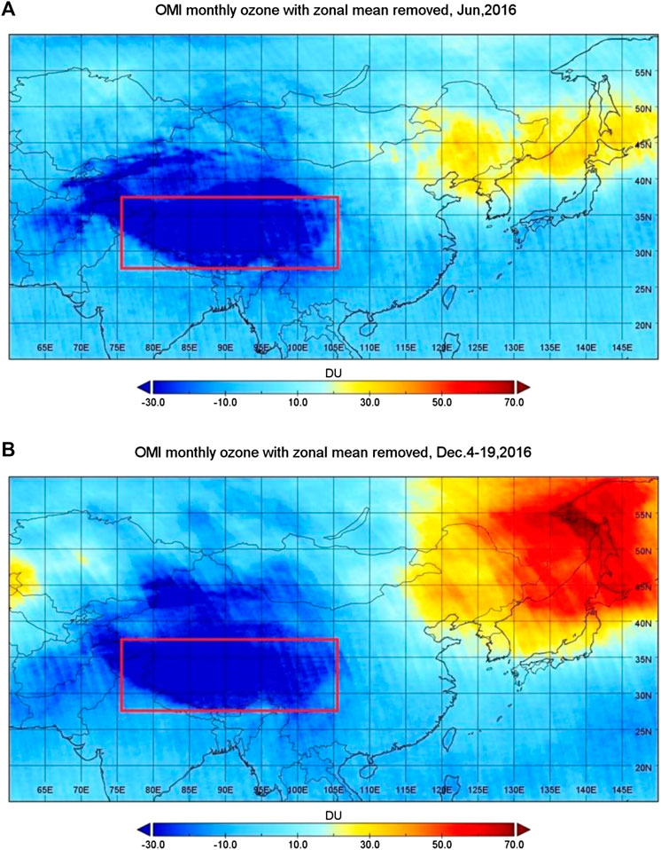
FIGURE 1. Spatial distribution of the ozone deficit over east Asia (A) in June 2016 and (B) in December 2016 (using data during 14–19 only). Data are from OMI measurement.

FIGURE 2

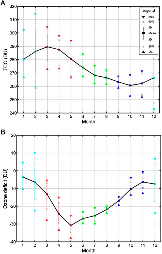
FIGURE 2. Seasonal variation of the monthly TCO mean over the TP (A) and the ozone deficit (B) using OMI data from October 2004 to February 2020.

Trend Analysis of Total Column Ozone in Different Latitudinal Zones near Tibetan Plateau Using Ensemble Empirical Mode Decomposition Method

MOD is a monthly zonal mean and gridded product constructed by merging individual SBUV/SBUV/2 (total and profile ozone) data sets, and it covers a period of ∼48°years since 1972. Considering MOD is a gridded data in 5 degree of zonal mean, we use these data over 30°N–35°N latitudinal zone in the TP and its trend is analyzed using the EEMD method. For comparison, the trends of TCO in the south of TP over 25°N–30°N and north of the TP over 35°N–40°N are also analyzed. Figure 3 shows the EEMD decomposition analysis of monthly TCO over the TP, with the right panels showing the components and the left panel showing the residual components of decomposition. To get a better view, R_i is plotted by adding (5 − i) × 205 (i = 1, 2, 3, 4, 5); the original monthly mean MOD data (green line) and final residual R₅ (red) are plotted by adding (5 × 205 + 80). Similarly, in the right panel, different components C_i are plotted by adding (5 − i) × 29 (i = 1, 2, 3, 4, 5). IMFs C_i represent the TCO variations with frequency from high to low. The amplitudes of IMFs represent the strength of TCO variations. The EEMD method can give IMF components, but the individual component cannot guarantee a well-defined physical meaning which is true for all decomposing methods, especially for the methods with an a priori basis (Huang et al., 1998). The rule for interpreting the physical significance of IMFs is based on the time scales. C₁ shows a fast oscillation while low amplitude with a time scale less than a month. C₂ and C₃ show strong oscillations with time scales of several months, and these two components can reflect the seasonal behavior of TCO. C₄ shows an oscillation with time scale of years, and C₅ shows little oscillation with even longer time scale. After IMFs are extracted, the final residual R₅ represents the TCO trend from EEMD analysis, and the monthly increase rates are calculated from the derivative of residual R₅. As shown in Figure 4, before 1996, the TCO all have negative trends, but the decrease rate gets smaller and then starts to increase after 1996. The peak of the positive increase trends occurs in ∼2000 over the latitudinal zone 30°N–35°N, which is slightly behind the faster recoveries over latitudinal zones of 25°N–30°N and 35°N–40°N. Such a recovery of ozone continues to 2011 in the latitudinal zone 30°N–35°N over the TP, but since 2012, the TCO shows a slightly decrease again. Since most studies found the pinpoint of the trend change occurred in 1996 (e.g., Li et al., 2020), the MOD data from 1979 to 1996 are kept as one period, and the period from 1997 to 2018 is treated as another one. Meanwhile, we broke the data from 1997 to 2018 into two other subperiods: 1997–2003 and 2004–2018, as the OMI TCO data date from 2004, so they can be compared with each other. In the following analysis, the annual trends will be calculated based on EEMD decomposition of MOD data during four periods (1979–1996, 1997–2018, 1997–2003, and 2004–2018). Using the monthly trend shown in Figure 4 to compute the annual mean ozone trend in the latitudinal zone 30°N–35°N, we got the mean annual trends with confidence interval at 95% confidence level which are −0.836 ± 0.233 DU/yr during 1979–1996, 0.021 ± 0.124 DU/yr during 1997–2018, 0.291 ± 0.056 DU/yr during 1997–2003, and −0.104 ± 0.14 DU/yr during 2004–2018. The trend during 1997–2018 confirms a positive but relatively small rate of increase after 1997, which is consistent with the conclusion from Li et al. (2020).

FIGURE 3

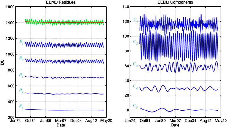
FIGURE 3. EEMD-based decomposition of TCO from MOD/NASA over 30°N–35°N latitudinal zone.

FIGURE 4

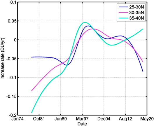
FIGURE 4. Monthly increase rates of TCO over 30°N–35°N latitudinal zone over the TP and its comparison to its south at 25°N–30°N and north at 35°N–40°N.

Trend Analysis of Ozone Deficit over Tibetan Plateau Using Ozone Monitoring Instrument Data from 2004 to 2019

Since MOD data only have the zonal mean of TCO, we used OMI measurements, which are available since 2004 to present, to analyze the trend of ozone deficit over the TP. Comparison of the zonal mean of OMI and MOD data in 30°N–35°N from 2004 to 2019 shows they agree very well, with the mean difference of 3.16 ± 1.76 DU (Figures 5A,B). Therefore, we can do similar analysis to the trend of TCO (and ozone deficit as well) as we already did using the MOD data, but with a shorter time series. Below we just focus on the trend of ozone deficit over the TP.

FIGURE 5

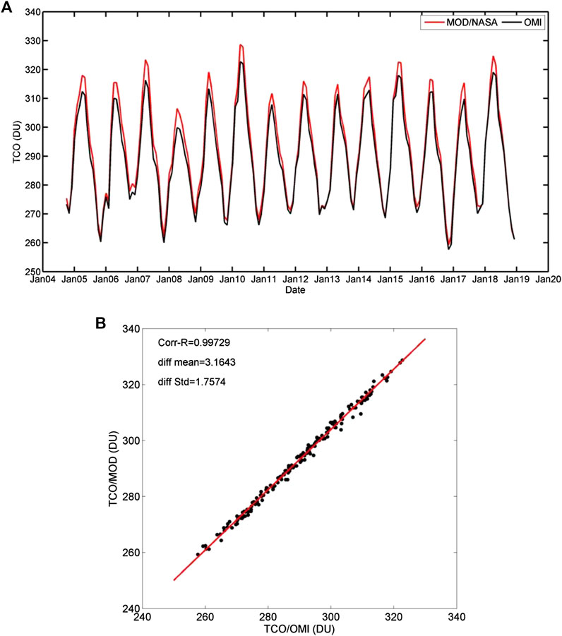
FIGURE 5. Variation of TCO zonal mean at 30–35°N from OMI from 2004 to 2019 and its comparison with MOD data in the same period (A). Scatter plot of the same OMI TCO vs. MOD data is shown in the lower panel (B).

Figure 6A shows the decompositions of ozone deficit over the TP. Since the IMFs C₂ and C₃ from EEMD-based decomposition reflect the seasonal behavior, we found a combination of C₂ and C₃ decomposed from OMI measurements can clearly present the ozone deficit seasonal variation. Compared to TCO, the combination of C₂ and C₃ from ozone deficit shows larger seasonal variation. The increase rates of TCO derived using residual R₅ are shown in Figure 6B. For comparison, the increase rate from TCO over the TP is also shown in Figure 6B. The trend of the TCO over the TP is similar to the trend of the zonal mean TCO in Figure 4 but has slight difference. TCO trend shows a continual recovery over the TP since 2005, with the peak of the increase appearing in 2010. The ozone deficit has a positive trend since 2009 and increases more rapidly after 2015. This indicates that the ozone increase rate over the TP is larger than the zonal mean since 2009. Using the monthly trend of TCO and ozone deficit (Figure 6B), we got the mean annual increase rate of TCO over the TP with confidence interval at 95% confidence level which is 0.377 ± 0.148 DU/yr during 2004–2019, while the mean annual increase rate of ozone deficit is 0.263 ± 0.437 DU/yr.

FIGURE 6

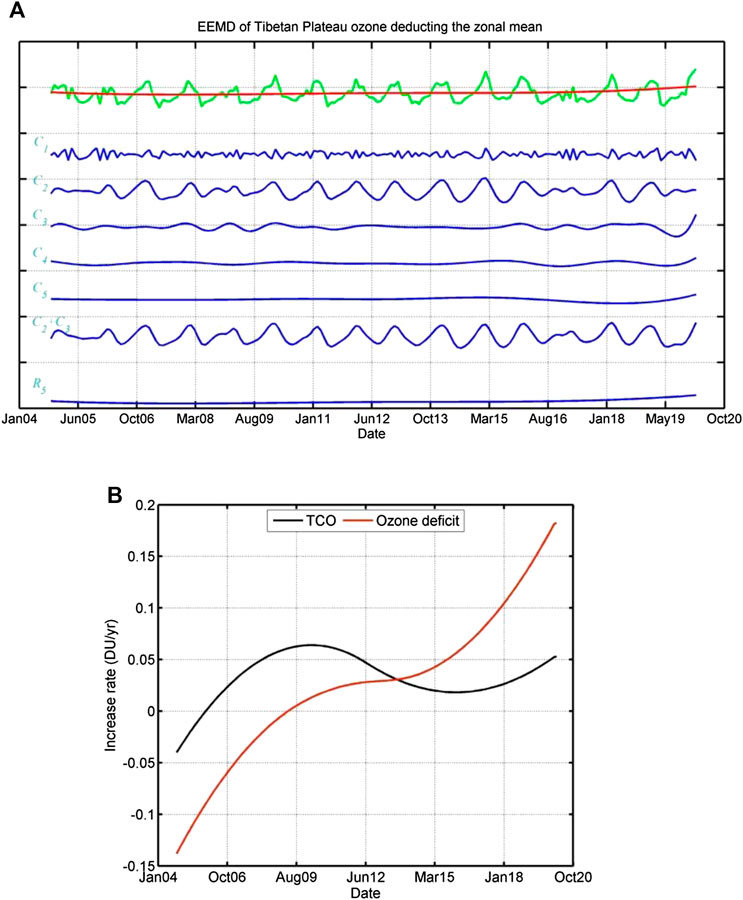
FIGURE 6. EEMD decompositions of ozone deficit over the TP (A) and the monthly increase rate derived from R5 (B). For comparison, the increase rate from TCO over the TP is also shown in the lower panel (B).

To better understand the difference of ozone trend over the TP, Figure 7 shows the ozone deficit in the early summer and winter, and the corresponding increase rates are shown in Figure 8. The low-ozone event usually occurs in May, but in the winter, it occurs mostly in December and February. It is evident that there is relatively faster ozone recovery over the TP than its zonal mean since 2009, with a faster increase in speed after 2015. The recovery of ozone in the winter season is faster than that in the summer season, and December takes the lead in this recovery.

FIGURE 7

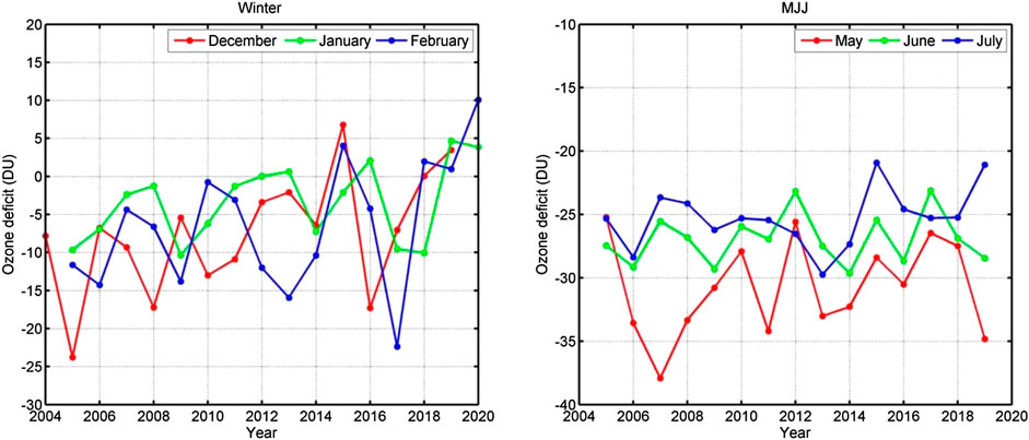
FIGURE 7. Variation of ozone deficit over the TP in winter (left) and early summer (right).

FIGURE 8

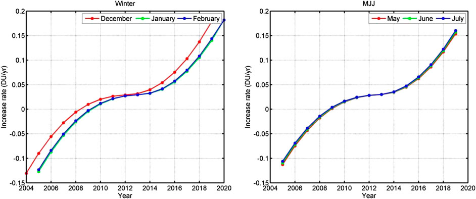
FIGURE 8. Trend of ozone deficit over the TP in winter (left) and early summer (right).

Low-Ozone Events over Tibetan Plateau from Ozone Monitoring Instrument and Ozone Mapping and Profiler Suite Data

Bian et al. (2006) reported the finding of low-ozone events in the December of 2003. From Figure 7, we found a few large ozone-deficit events in February, May, and December 2004 and February 2019. Considering the ozone deficits in December 2016 and February 2017 are extremely lower than others, as well as OMI and OMPS both have observations in these two periods, we plot the daily TCO change over the TP in these two periods (two left panels in Figure 9) using measurements from the OMI and OMPS. The daily ozone products from the OMI and OMPS agree very well, and both shows a lasting low-ozone event of about two weeks in the December of 2016. By removing the zonal mean ozone, the daily TCO deficit (two right panels in Figure 9) more clearly show the low-ozone days in these two months. Further analysis of low-ozone events in February (2006, 2009, 2012, and 2013), May (2006–2008, 2011, 2013, 2014, and 2019), and December (2005, 2008, and 2010) has been done based on the daily TCO deficit. According to the statistics of monthly ozone deficit (shown in Figure 2B), we choose the 10 percentile as reference, which means −34 DU for May, −16 DU for February, and −17 DU for December, to count for the extreme low-ozone days below these reference values. Selection of such thresholds is little arbitrary, and the number of the days representing how long the low-ozone event lasts is sensitive to these thresholds. The detailed statistics of these selected months are listed in Table 1. The low-ozone event in May is deeper than that in February and December. The number of extreme low-ozone days is around 17 in May which is equivalent to that in December but longer than that in February; 2015 is the only year in which the trends of ozone deficit in all selected six months are positive. Compared to the low-ozone days in the summer that are mainly controlled by the transport from the troposphere to stratosphere over the TP (e.g., Zhou et al., 2006; Tian et al., 2008), the mechanism of low-ozone days is the winter is more complex (e.g., Li et al., 2020).

FIGURE 9

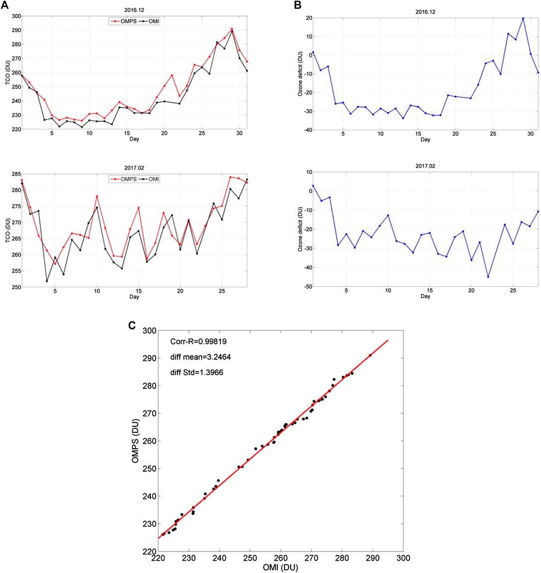
FIGURE 9. Examples of extreme low-ozone events over the TP. (A) Daily TCO (two left panels) and the ozone deficit (two right panels) from OMI in December 2016 and February 2017; (B) scatter plot of OMI daily TCO vs. OMPS daily TCO.

TABLE 1

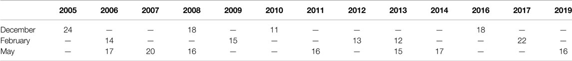
TABLE 1. Number of days when the OMI daily TCO deficit is below −34 DU for May, below −16 DU for February, and below −17 DU for December.

Conclusion

To better understand the trend of ozone over the Tibetan Plateau, we used ozone measurement from OMI/Aura from 2004 to 2019 and the EEMD method to analyze the trends of total column O₃ and the ozone deficit after removing the corresponding zonal mean TCO over the TP. Analysis of the zonal mean TCO trends using the merged ozone data from NASA from 1978 to 2019 shows a slight recovery of ozone during 1996–1997; however, after 2013, only the north of the TP shows an increase trend, but the zonal mean between 30°N and 40°N shows a decrease trend. The mean annual increase rates over the latitudinal zone 30–35°N are −0.836 ± 0.233 DU/yr during 1979–1996, 0.291 ± 0.056 DU/yr during 1997–2003, and −0.104 ± 0.14 DU/yr during 2004–2018. The trend of 0.021 ± 0.124 DU/yr during 1997–2018 confirms a positive but relatively small rate of increase after 1997.

Comparison of the zonal mean ozone from 2004 to 2019 from the OMI product with the merged ozone data from NASA, as well as comparison of TCO over the TP from the OMI and the most recent measurements from OMPS on S-NPP, shows that they agree with each other quite well. Using OMI data, we examined the trend of ozone over the TP and the trend of ozone deficit in different seasons. We found that the TCO over the TP shows a consistent increase trend from 2005 to 2019, and the ozone deficit over the TP has a positive trend since 2009 and an even more rapid increase trend after 2015, with a larger increase in the winter season summer. It indicates that the ozone increase rate over the TP is larger than the zonal mean since 2009. This finding of more and faster increase of ozone over the TP relative to the zonal mean suggests the possibility of the decrease of the UV radiation to the ground surface over the TP, which will benefit to human skin health and biosphere there. Further analysis of the low-ozone events in winter and early summer from 2004 to 2019 shows that the low-ozone event in May is much deeper and lasts longer than that in February. Overall, trend analysis from OMI measurements shows positive increase rates during the past 2 decades over the TP. The mean annual increase rates over TP are 0.377 DU/yr for TCO and 0.263 DU/yr for ozone-deficit events during 2004–2019. There are many causes for this trend, such as a local photochemical reaction and transformation. Simulation from the atmospheric chemical model and in situ observations will be used to learn the mechanism of ozone variation in the future study.

Data Availability Statement

The data sets generated for this study are available on request to the corresponding author.

Author Contributions

MZ and XX wrote the paper. MZ performed the data curation and visualization. XX and MZ did formal analysis, the result investigation, and paper editing. ZW supplied code of EEMD. CY was responsible for data preprocessing.

Funding

This research was funded by the National Natural Science Foundation of China, grant number 41771390.

Conflict of Interest

XX was employed by the company Science Systems and Applications, Inc.

The remaining authors declare that the research was conducted in the absence of any commercial or financial relationships that could be construed as a potential conflict of interest.

Acknowledgments

We are grateful to NASA GESDISC DATA for providing OMI and OMPS total column data and also many thanks to NASA Goddard Space Flight Center for providing SBUV MOD data used in this study.

References

Bai, K., Liu, C., Shi, R., and Gao, W. (2015). Comparison of Suomi-NPP OMPS total column ozone with Brewer and Dobson spectrophotometers measurements. Front. Earth Sci. 9 (3), 369–380. doi:10.1007/s11707-014-0480-5

CrossRef Full Text | Google Scholar

Bak, J., Liu, X., Kim, J., Haffner, D., Chance, K. V., Yang, K., et al. (2017). Characterization and correction of OMPS nadir mapper measurements for ozone profile retrievals. Atmos. Meas. Tech. 10 (11), 4373–4388. doi:10.5194/amt-10-4373-2017.

CrossRef Full Text | Google Scholar

Bhartia, P. K., McPeters, R. D., Flynn, L. E., Taylor, S., Kramarova, N. A., Frith, S., et al. (2013). Solar Backscatter UV (SBUV) total ozone and profile algorithm. Atmos. Meas. Tech. 6 (10), 2533–2548. doi:10.5194/amt-6-2533-2013.

CrossRef Full Text | Google Scholar

Bian, J. C., Wang, G. H., Chen, H. B., Qi, D. L., Lü, D. R., and Zhou, X. J. (2006). Ozone mini-hole occurring over the Tibetan Plateau in December 2003. Chin. Sci. Bull. 51 (7), 885–888. doi:10.1007/s11434-006-0885-y.

CrossRef Full Text | Google Scholar

Burrows, J. P., Weber, M., Buchwitz, M., Rozanov, V., Ladstätter-Weißenmayer, A., Richter, A., et al. (1999). The global ozone monitoring experiment (GOME): mission concept and first scientific results. J. Atmos. Sci. 56 (2), 151–175. doi:10.1175/1520-0469(1999)056<0151:tgomeg>2.0.co;2.

CrossRef Full Text | Google Scholar

Chen, S. B., Zhao, L., and Tao, Y. L. (2016). Stratospheric ozone change over the Tibetan Plateau. Atmos. Pollut. Res. 8 (3), 528–534. doi:10.1016/j.apr.2016.11.007.

CrossRef Full Text | Google Scholar

DeLand, M. T., Taylor, S. L., Huang, L. K., and Fisher, B. L. (2012). Calibration of the SBUV version 8.6 ozone data product, Atmos. Meas. Tech. 5 (11), 2951–2967. doi:10.5194/amt-5-2951-2012.

CrossRef Full Text | Google Scholar

Dobson, G. M. B. (1968). Forty years’ research on atmospheric ozone at Oxford: a history. Appl. Optics 7 (3), 387. doi:10.1364/AO.7.000387.

CrossRef Full Text | Google Scholar

Flynn, L., Long, C., Wu, X., Evans, R., Beck, C. T., Petropavlovskikh, I., et al. (2014). Performance of the ozone mapping and profiler suite (OMPS) products. J. Geophys. Res. Atmos. 119 (10), 6181–6195. doi:10.1002/2013JD020467.

CrossRef Full Text | Google Scholar

Frith, S. M., Kramarova, N. A., Stolarski, R. S., McPeters, R. D., Bhartia, P. K., and Labow, G. J. (2014). Recent changes in total column ozone based on the SBUV version 8.6 merged ozone data set. J. Geophys. Res. Atmos. 119 (16), 9735–9751. doi:10.1002/2014JD021889.

CrossRef Full Text | Google Scholar

Guo, D., Su, Y. C., Zhou, X. J., Xu, J. J., Shi, C. H., Liu, Y., et al. (2017). Evaluation of the trend uncertainty in summer ozone valley over the Tibetan plateau in three reanalysis datasets. J. Meteor. Res. 31 (2), 431–437. doi:10.1007/s13351-017-6058-x

CrossRef Full Text | Google Scholar

Harris, N. R. P., Kyrö, E., Staehelin, J., Brunner, D., Andersen, S.-B., Godin-Beekmann, S., et al. (2008). Ozone trends at northern mid- and high latitudes—a European perspective. Ann. Geophys. 26 (5), 1207–1220. doi:10.5194/angeo-26-1207-2008.

CrossRef Full Text | Google Scholar

Huang, N. E., Shen, Z., Long, S. R., Wu, M. C., Shih, H. H., Zheng, Q., et al. (1998). The empirical mode decomposition and the Hilbert spectrum for nonlinear and non-stationary time series analysis. Proc. R. Soc. London. Ser. A 454 (1971), 903. doi:10.1098/rspa.1998.0193

CrossRef Full Text | Google Scholar

Huang, N. E., and Wu, Z. (2008). A review on Hilbert-Huang transform: method and its applications to geophysical studies. Rev. Geophys. 46 (2), RG2006. doi:10.1029/2007rg000228

CrossRef Full Text | Google Scholar

Kramarova, N. A., Frith, S. M., Bhartia, P. K., McPeters, R. D., Taylor, S. L., Fisher, B. L., et al. (2013). Validation of ozone monthly zonal mean profiles obtained from the version 8.6 Solar Backscatter Ultraviolet algorithm. Atmos. Chem. Phys. 13 (14), 6887–6905. doi:10.5194/acp-13-6887-2013

CrossRef Full Text | Google Scholar

Kramarova, N., Nash, E. R., Newman, P. A., Bhartia, P. K., McPeters, R. D., Rault, D. F., et al. (2014). Measuring the Antarctic ozone hole with the new ozone mapping and profiler suite (OMPS). Atmos. Chem. Phys. 14 (5), 2353–2361. doi:10.5194/acp-14-2353-2014

CrossRef Full Text | Google Scholar

Kroon, M. W., Petropavlovskikh, I., Shetter, R. E., Hall, S. R., Ullmann, K., Veefkind, J. P., et al. (2008). OMI total ozone column validation with Aura-AVE CAFS observations. J. Geophys. Res. 113, D15. doi:10.1029/2007JD008795

CrossRef Full Text | Google Scholar

Labow, G. J., McPeters, R. D., Bhartia, P. K., and Kramarova, N. A. (2013). A comparison of 40 years of SBUV measurements data from the Dobson/Brewer network, J. Geophys. Res. Atmos. 118 (13), 7370–7378. doi:10.1002/jgrd.50503

CrossRef Full Text | Google Scholar

Li, Y., Chipperfield, M. P., Feng, W., Dhomse, S. S., Pope, R. J., Li, F., et al. (2020). Analysis and attribution of total column ozone changes over the Tibetan Plateau during 1979–2017. Atmos. Chem. Phys. 20 (14), 8627–8639. doi:10.5194/acp-20-8627-2020

CrossRef Full Text | Google Scholar

Liu, C. X., Liu, Y., Cai, Z. N., Gao, S. T., Bian, J. C., Liu, X., et al. (2009). Dynamic formation of extreme ozone minimum events over the Tibetan Plateau during northern winters 1987-2001. J. Geophys. Res. 115, D18311. doi:10.1029/2009JD013130

CrossRef Full Text | Google Scholar

Liu, Y., Li, W. L., and Zhou, X. J. (2001). Prediction of the trend of total column ozone over the Tibetan Plateau. Sci. China. 44 (l), 385–389. doi:10.1007/bf02912010

CrossRef Full Text | Google Scholar

Liu, X., Bhartia, P. K., Chance, K., Spurr, R. J. D., and Kurosu, T. P. (2010). Ozone profile retrievals from the ozone monitoring instrument. Atmos. Chem. Phys. 10 (5), 2521–2537. doi:10.5194/acp-10-2521-2010

CrossRef Full Text | Google Scholar

McPeters, R. D., Bhartia, P. K., Haffner, D., Labow, G. J., and Flynn, L. (2013). The version 8.6 SBUV ozone data record: an overview. J. Geophys. Res. Atmos. 118 (14), 8032–8039. doi:10.1002/jgrd.50597

CrossRef Full Text | Google Scholar

McPeters, R., Frith, S., Kramarova, N., Ziemke, J., and Labow, G. (2019). Trend quality ozone from NPP OMPS: the version 2 processing. Atmos. Meas. Tech. 12, 977–985. doi:10.5194/amt-12-977-2019

CrossRef Full Text | Google Scholar

Pawson, S., Steinbrecht, W., Charlton-Perez, A. J., Fujiwara, M., Karpechko, A. Y., Petropavlovskikh, I., et al. (2014). “Update on global ozone: past, present, and future,” in Scientific assessment of ozone depletion: 2014, global ozone research and monitoring project (Geneva, Switzerland:World Meteorological Organization/UNEP), Chap. 2, Report No. 55.

Google Scholar

Rodgers, C. D. (1976). Retrieval of atmospheric temperature and composition from remote measurements of thermal radiation. Rev. Geophys. 14 (4), 609–624. doi:10.1029/RG014i004p00609

CrossRef Full Text | Google Scholar

Richter, A., Wittrock, F., Weber, M., Beirle, S., Kühl, S., Platt, U., et al. (2005). GOME observations of stratospheric trace gas distributions during the splitting vortex event in the Antarctic winter of 2002. Part I: measurements. J. Atmos. Sci. 62, 778–785. doi:10.1175/JAS-3325.1

CrossRef Full Text | Google Scholar

Schoeberl, M. R., Douglass, A. R., Hilsenrath, E., Bhartia, P. k., Beer, R., Waters, J. W., et al. (2006). Overview of the EOS Aura mission. Geoscience and remote sensing. IEEE Trans. 44, 1066–1074. doi:10.1109/TGRS.2005.861950

CrossRef Full Text | Google Scholar

Solomon, S. (1999). Stratospheric ozone depletion: a review of concepts and history. Rev. Geophys. 37, 275–316. doi:10.1029/1999RG900008

CrossRef Full Text | Google Scholar

Staehelin, J., Renaud, A., Bader, J., McPeters, R., Viatte, P., Hoegger, B., et al. (1998). Total ozone series at Arosa (Switzerland): homogenization and data comparison, J. Geophys. Res. Atmos. 103, 5827–5841. doi:10.1029/97JD02402

CrossRef Full Text | Google Scholar

Tian, W. S., Chipperfield, M. P., and Huang, Q. (2008). Effects of the Tibetan Plateau on total column ozone distribution. Tellus B 60, 622–635. doi:10.1111/j.1600-0889.2008.00338.x

CrossRef Full Text | Google Scholar

Veefkind, J. P., De Haan, J., Brinksma, E., Kroon, M., and Levelt, P. (2006). Total ozone from the ozone monitoring instrument (OMI) using the OMI-DOAS technique. IEEE T. Geosci. Remote. 44, 1239–1244. doi:10.1109/tgrs.2006.871204

CrossRef Full Text | Google Scholar

Wagner, T., Leue, C., Pfeilsticker, K., and Platt, U. (2001). Monitoring of the stratospheric chlorine activation by Global Ozone Monitoring Experiment (GOME) OClO measurements in the austral and boreal winters 1995 through 1999. J. Geophys. Res. Atmos. 106, 4971–4986. doi:10.1029/2000JD900458

CrossRef Full Text | Google Scholar

Weber, M., Coldewey-Egbers, M., Fioletov, V. E., Frith, S. M., Wild, J. D., Burrows, J. P., et al. (2018). Total ozone trends from 1979 to 2016 derived from five merged observational datasets—the emergence into ozone recovery. Atmos. Chem. Phys. 18, 2097–2117. doi:10.5194/acp-18-2097-2018

CrossRef Full Text | Google Scholar

Wu, Z. H., and Huang, N. E. (2009). Ensemble empirical mode decomposition: a noise-assisted data analysis method. Adv. Adapt. Data Anal. 01 (01), 1–41. doi:10.1142/s1793536909000047

CrossRef Full Text | Google Scholar

Wu, Z. H., Huang, N. E., Long, S. R., and Peng, C. K. (2007). On the trend, detrending, and variability of nonlinear and nonstationary time series. Proc. Natl. Acad. Sci. U.S.A. 104 (38), 14889–14894. doi:10.1073/pnas.0701020104

CrossRef Full Text | Google Scholar

Wu, Z. H., Huang, N. E., Wallace, J. M., Smoliak, B. V., and Chen, X. (2011). On the time-varying trend in global-mean surface temperature. Clim. Dynam. 37 (3), 759–773. doi:10.1007/s00382-011-1128-8

CrossRef Full Text | Google Scholar

Xiong, X. Z., Houweling, S., Wei, J. K., Maddy, E., Sun, F. Y., and Barnet, C. (2009). Methane plume over South Asia during the monsoon season: satellite observation and model simulation. Atmos. Chem. Phys. 9, 783–794. doi:10.5194/acp-9-783-2009

CrossRef Full Text | Google Scholar

Xu, W. Y., Lin, W. L., Xu, X. B., Tang, J., Huang, J. Q., Wu, H., et al. (2016). Long-term trends of surface ozone and its influencing factors at the Mt. Waliguan GAW station, China–part 1: overall trends and characteristics. Atmos. Chem. Phys. 16, 6191–6205. doi:10.5194/acp-16-6191-2016

CrossRef Full Text | Google Scholar

Xu, W. Y., Xu, X. B., Lin, M. Y., Lin, W. L., Tarasick, D., Tang, J., et al. (2018). Long-term trends of surface ozone and its influencing factors at the Mt. Waliguan GAW station, China–part 2: the roles of anthropogenic emissions and climate variability. Atmos. Chem. Phys. 18, 773–798. doi:10.5194/acp-18-773-2018

CrossRef Full Text | Google Scholar

Ye, D. Z., and Wu, G. X. (1998). The role of the heat source of the Tibetan Plateau in the general circulation. Meteorol. Atmos. Phys. 67, 181–198. doi:10.1007/bf01277509

CrossRef Full Text | Google Scholar

Zhang, J. K., Tian, W. S., Xie, F., Tian, H. Y., Luo, J. L., Zhang, J., et al. (2014). Climate warming and decreasing total column ozone over the Tibetan Plateau during winter and spring. Tellus B 66 (1), 23415. doi:10.3402/tellusb.v66.23415

CrossRef Full Text | Google Scholar

Zhou, X. J., Li, W. L., Chen, L. X., and Liu, Y. (2006). Study on ozone change over the Tibetan plateau. J. Meteor. Res. 20 (2), 129–143.

Google Scholar

Zou, H. (1996). Seasonal variation and trends of TOMS ozone over Tibet. Geophys. Res. Lett. 23, 1029–1032. doi:10.1029/96gl00767

CrossRef Full Text | Google Scholar

Zou, M. M., Xiong, X. Z., Wu, Z. H., Li, S. S., Zhang, Y., and Chen, L. F. (2019). Increase of atmospheric methane observed from space-borne and ground-based measurements. Rem. Sens. 11, 964. doi:10.3390/rs11080964.

CrossRef Full Text | Google Scholar