How Continuous Are the “Relict” Landscapes of Southeastern Tibet?

Introduction

The South Eastern margin of the Tibetan Plateau has grown during the last 50 million years (Myr) through a combination of geodynamic processes: eastwards extrusion driven by motion on strike slip faults (Tapponnier et al., 1982); crustal thickening induced by lower crustal flow (Clark and Royden, 2000; Copley, 2008); slab rollback below its eastern margin (Sternai et al., 2012); and general shortening and crustal thickening due to collision of the Indian plate and Eurasia (Yang et al., 2015; Tan et al., 2019). In order to assess how these mechanisms have contributed to the current topography, it is crucial to determine rock uplift in space and time, commonly, through geochronology and geomorphology. One of the key geomorphic features that has been used to aid in this mapping are pervasive low-relief, high-elevation topography that is separated by incised canyons with high relief. These low-relief surfaces, that have areas typically 10 s of km², have been identified across SE Tibet and decrease gradually in elevation from ∼5 km to less than 1 km over a lengthscale of approximately 1,000 km (Clark et al., 2006). The relief averaged over 5 km within these low-relief landscapes is typically less than 1 km. This landscape has been argued to result from an increase in rock uplift rate (Clark and Royden, 2000). Rivers respond to rock uplift by steepening and these steepened sections incise backwards into slowly eroding areas that have not yet equilibrated to the new rock uplift rate. These patches of low-relief areas are therefore assumed to be parts of the landscape that have not yet adjusted to the new rock uplift rate. The deeply incised canyons, however, have responded to this change in rock uplift rate.

By mapping the extent of these uplifted surfaces, the region that experienced a change in rock uplift can be estimated. In addition, if the difference between erosion rates on the surfaces and in the canyons can be estimated, the time required for these surfaces to reach their current elevation above the surrounding canyons can be inferred.

For example, Clark and Royden (2000) proposed that a low-viscosity channel in the lower crust accommodates the movement of crustal material from high pressures below the plateau to lower pressures away from the plateau. This mechanism simplifies to a diffusion equation in which elevation diffuses from the plateau leading to spatial and temporal variations in surface uplift (England and Molnar, 1990). Because crustal thickening occurs due to flow in the lower crust, the surface is uplifted but deformation is small and there is limited lateral transport of the surfaces. If the erosion rates on the low-relief surfaces are assumed to be close to zero, mapping these surfaces and dating incision can constrain the uplift rate history and the effective viscosity of the low-viscosity channel (Clark and Royden, 2000; Schoenbohm et al., 2004; Clark et al., 2006; Ouimet et al., 2010; Liu-Zeng et al., 2018). Furthermore, this scenario leads to an overall increase in topographic elevation through time. Throughout this study, we will refer to the idea that the low-relief surfaces are remnants of a relict low-relief landscape that has been dissected with minimal drainage network reorganization as Hypothesis 1 and stress that this is a simplification of the proposed model (Figure 1).

FIGURE 1

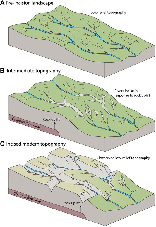
FIGURE 1. Hypothesis 1. (A) Before the onset of rock uplift across SE Tibet, Hypothesis 1 proposes that there was a low-relief landscape with low erosion rates. (B) Due to lower-crustal channel flow, rock uplift rates increased and rivers incised into the low-relief landscape. (C) Remnants of the low-relief landscape are preserved today and have not been removed by erosion. Therefore, the low-relief remnants can potentially be used to map geodynamic processes.

Importantly, the assumption that enables low-relief high-elevations surfaces to map rock uplift rates is that erosion rates on the surfaces were low prior to the change in rock uplift and have not changed since this adjustment, or at least that changes in erosion rate can be quantified. Several factors, however, may lead to temporal changes in erosion rate across low-relief surfaces as they are uplifted and some of these factors may even form these surfaces: the surfaces may experience changing elevation-dependent climatic conditions as they increase in elevation leading to changes in vegetation and changes in weathering processes that will influence erosion rates (Hales and Roering, 2007; Roering et al., 2010; Schaller et al., 2018); climate may change regionally due to the changes in topography resulting from surface uplift leading to changes in the patterns, in space and time, of rainfall (Molnar et al., 2010; Ferrier, et al., 2013; Scherler et al., 2017); Quaternary global climate change may have resulted in enhanced or reduced erosion across some of these surfaces (Egholm et al., 2009; Fox et al., 2015a; Egholm et al., 2017).

Recently, however, a model has been proposed in which the surfaces are formed by changes in erosion rate but no significant change in rock uplift rate driven by dynamic adjustment of the drainage networks due to tectonic strain (Hallet and Molnar, 2001; Yang et al., 2015). In this scenario, low slope rivers with large upstream drainage area and equilibrated channel steepness, lose upstream drainage area, reducing channel steepness and thus erosion rate. Once this erosion rate is reduced, the landscape is out of equilibrium with the regional rock uplift rate and would be advected upwards, while surrounding channels continue to erode at the rock uplift rate. As this low-relief surface is being uplifted, rivers incise into the boundaries of these isolated surfaces. In this scenario, the general features of the topography may stay relatively constant, with new low-relief surfaces forming and being lost to erosion through time. Throughout this study we will refer to this model as Hypothesis 2 (Figure 2). This hypothesis remains controversial and it is currently unclear whether the low-relief surfaces are relicts of a remnant topography and can be used to map rock uplift rates in space and time. In particular, Whipple et al. (2017) argued that the low-relief upland landscape patches are approximately co-planar and decrease in elevation from the northwest to the southeast and that variability in the elevations of bounding knickpoints is expected in natural landscapes. It remains unclear how much variability is expected and how much is due to regional geodynamics or the expected change in elevation along the trunk river profiles. Willett (2017) argued that Whipple et al. (2017a) only analyzed topography at the 100 –1,000 km scale but did not look at individual drainage basins. Furthermore, Willett (2017) suggested that the topography might be consistent with incision into a pre-existing landscape if spatially variable rock uplift is accounted for “pending a detailed study”. In response, Whipple et al. (2017b) agreed that diagnostic criteria in landscape evolution are not easily determined and that it is important to examine multiple criteria in a regional context. Whipple et al. (2017b) also maintained that the low-relief topography was co-planar and defines an upper envelope to the topography and thus the topography of SE Tibet does result from incision into a pre-existing low-relief landscape. Importantly, these studies use a stream-power framework and we will adopt these same assumptions here. For simplicity, we have distilled the two concepts into endmember hypotheses. In reality, it is important to note that neither hypothesis is mutually exclusive nor collectively exhaustive (Whipple et al., 2017a; Whipple et al., 2017b; Willett, 2017).

FIGURE 2

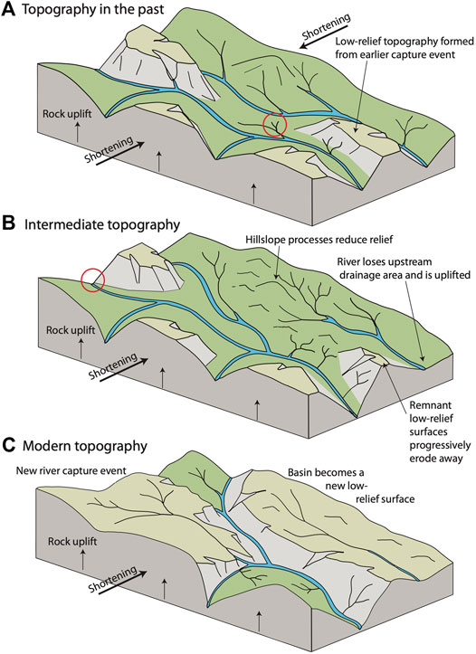
FIGURE 2. Hypothesis 2. (A) After a topography had developed across SE Tibet, Hypothesis 2 proposes there would have been some low-relief landscapes due to drainage reorganization. (B) During ongoing drainage reorganization driven by shortening perpendicular to major rivers, the tributary circled in (A) captures the upper river. The associated loss in upstream drainage area reduces the erosion rate of the river leading to surface uplift. Hillslope processes continue to erode hillslopes however the river has lost the ability to incise, leading to a reduction in topographic relief. Low-relief surfaces from previous capture events are eaten away by erosion. (C) The basin that lost upstream drainage area continues to have less and less relief and is eaten away by erosion. A capture event upstream of the red circle in (B) leads to the beginning of new low-relief topography. This process is continuous and leads to the lowest-relief landscape being preserved for short amounts of time at the highest elevations. Therefore, the modern topography reveals a snapshot of this process and patches of low-relief landscape at high elevations are not remnant of a pervasive low-relief landscape.

To test these hypotheses and to help diagnose how low-relief, high-elevation topography may form, we utilize linear inverse methods to interpolate a hypothetical topographical surface between the low-relief high-elevation surfaces (Fox, 2019). Importantly, we are not simply testing how co-planar the low-relief high-elevation surfaces are, but ensuring that the topographical surface must follow slope-area relationships with variable channel steepness. Furthermore, we account for the fact that the topographic surface might have been warped by geodynamic processes or offset by brittle faulting. If a topographical surface can be found with “relatively uniform” normalized rock uplift rate, u*, this supports the hypothesis that SE Tibet was a low-relief low-elevation surface that has been uplifted and dissected. Here “relatively uniform” would mean that the inferred normalized rock uplift rate between the low-relief surfaces is similar to the normalized rock uplift rate values observed on the low-relief surfaces. Alternatively, if a surface with large variations in normalized rock uplift rate is found, even without the inclusion of the incised portions of the landscape, this is inconsistent with Hypothesis 1 and instead supports Hypothesis 2. In this way, our approach does not explicitly test Hypothesis 2, but if a low-relief paleotopography can be constructed, the importance of Hypothesis 2 is reduced.

Using Fluvial Metrics to Test the Hypotheses

Fluvial geomorphology, and the associated metrics based on the stream power model, provide insight into how landscapes respond to changes in tectonic forcing (Howard, 1994). The rate of change of river long-profiles, dz/dt, increases with rock uplift rate, u, and decreases with erosion rate, e. In the stream power model, erosion rate is proportional to the upstream drainage area, A and the local channel slope, S, raised to the powers of m and n respectively. The constant of proportionality is the erodibility, K, which encompasses bedrock strength, bedload, hydraulic parameters and climate. Therefore,

$\frac{\text{dz}}{\text{dt}}=\text{u}-{\text{ KA}}^m{\text{S}}^n(1)$

and, if dz/dt = 0, u = KA^mSⁿ. Because K cannot be inferred directly from a landscape, it is common to measure the normalized channel steepness k_sn=A^m/nS, where m/n = 0.3–0.8 (Mudd et al., 2018) directly from a digital elevation model (DEM) which provides an estimate of the uplift rate at steady state (Kirby and Whipple, 2012). We build on previous work that has used the stream power model to debate the origin of the topography of SE Tibet and assume n = 1 and discuss the implications of this assumption in Dicussion (Yang et al., 2015; Whipple et al. 2017a; Whipple et al., 2017b; Willett, 2017). A value of m = 0.45 has been determined for parts of SE Tibet and we will use this same value (Kirby et al., 2003; Ouimet et al., 2009; Yang et al., 2015). The normalized channel steepness index approach to asses the topography of SE Tibet assumes steady state rock uplift, a fixed drainage network and a uniform K value in space and time. An advantage of this approach is that normalized channel steepness values can be calculated for every river node in a large digital elevation model, and it is therefore easy to interpret spatial patterns in the data (Kirby et al., 2003). In this respect, this approach is ideal to exploit the large topographic datasets available. A potential limitation is that by calculating slope from a DEM, noise in the dataset is amplified resulting in maps that can be hard to interpret. Therefore, averaging and smoothing is required to interpret normalized channel steepness maps. If low-relief surfaces were part of a continuous and former steady-state surface developed under relatively spatially constant rock uplift rate, similar channel steepness values would be expected across all low-relief surfaces and this has been argued by Whipple et al. (2017a). This would support Hypothesis 1. It is worth noting that Whipple et al. (2017b) do expect some variability in the form of the low-relief surface due to drainage re-arrangement and expected spatial variations in initial conditions, forcing mechanisms, and landscape response.

If the rock uplift rate increases, a fluvial knickpoint will form at the baselevel and propagate upstream at a speed given by KA^m, if n = 1. Therefore, the response time at a specific location, x, in the landscape from the baselevel, x_b, is given by

$\text{τ}={\displaystyle \underset{{\text{x}}_{\text{b}}}{\overset{\text{x}}{\int }}\frac{{\text{dx}}^{\prime }}{KA{\left(x^{\prime }\right)}^m}{\text{dx}}^{\text{′}}} (2)$

As with the normalized channel steepness, K is often unknown and thus it is useful to use a modified response time, or $\chi$ (Perron and Royden, 2012), that can be written as $\chi$ = A₀^m Kτ. The integral quantity $\chi$ can be used to identify whether drainage divides are stable with the assumption being that if baselevel falls at a confluence, a steepened section of a river profile, or knickpoint, will propagate upstream, potentially to a shared drainage divide. If knickpoints arrive at the drainage divide at different times, erosion rates will be different and the divide will migrate (Willett et al., 2014). Divide migration rate is expected to be relatively slow (Whipple et al., 2017c) but, in some cases, can be faster than the rate of knickpoint retreat (Schwanghart and Scherler, 2020) Therefore, $\chi$ values either side of drainage divides should be similar if divides are stationary but may be different if divides are moving. It is important to bear in mind that the interpretation of $\chi$ maps assumes spatially uniform K values and rock uplift rate, and that spatial variability in K or rock uplift rates may lead to stationary divides that have different large $\chi$ differences. As with maps of channel steepness, entire drainage networks can be analyzed simultaneously without the requirement that the erodibility is known. Maps of $\chi$, however, have no information about the normalized channel steepness of river profiles. Large differences in $\chi$ across drainage divides would support Hypothesis 2, but is also expected in Hypothesis 1 due to drainage capture (Clark et al., 2004).

To provide information on relative channel steepness values, $\chi$ can be plotted as a function of elevation for rivers and the slope of this curve is proportional to normalized channel steepness (Perron and Royden, 2012; Goren et al., 2014; Mudd et al., 2014). This is because, at steady state with n = 1, Eq. 1 reduces to:

$\text{z}\left(\text{x}\right)=\text{z}\left({\text{x}}_{\text{b}}\right)+\left(\frac{\text{u}}{{\text{KA}}_0^{\text{m}}}\right)\text{χ }(3)$

and the normalized rock uplift rate is u*= u/A₀^mK, which is also proportional to the normalized channel steepness, i.e., u* = k_sn/A₀^m. We discuss the implications of the n = 1 and highlight how we can account for nonlinearity in the discussion. Furthermore, rivers that have experienced similar rock uplift rate histories should have similar forms as knickpoints will have traveled to similar $\chi$ values (Ma et al., 2020). Importantly, this provides an additional means to test Hypothesis 1 as the $\chi$-elevation relationship of the low-relief surfaces should be the same. The additional information that is obtained by using $\chi$-elevation plots is that the $\chi$ values of the knickpoints separating the low-relief surfaces from the incising canyons should be similar across much of the landscape if Hypothesis 1 is correct. However, spatial variability in the geodynamics driving incision into the low-relief surface may distort $\chi$-elevation relationships making this analysis complicated. A disadvantage of extracting channel profiles and plotting the topographic data in this form is that it is much harder to interpret spatial patterns in the data. Furthermore, channels must be extracted for analysis and this prevents entire datasets being analyzed simultaneously. $\chi$-elevation plots have been used to argue in favor of both Hypothesis 1 and Hypothesis 2 (Yang et al., 2015; Whipple et al., 2017a; Whipple et al., 2017b; Willett, 2017).

methods

Our approach is based on the normalized analytical, steady state stream power model but allows for spatial variations in u* and surface uplift (S.U.) after the formation of the low-relief landscape. In this way, we adopt the same sets of assumptions that are the basis for the ongoing debate about the origin of the topography of SE Tibet and attempt to highlight why there is ongoing debate. If u* and S.U. vary in space, we can write a discrete version of Eq. 1 for a node in a DEM along a channel,

$z_i=z_j+\left({\chi }_i-{\chi }_j\right)u_j^{\ast }+S.U{.}_i(4)$

where the ith pixel is upstream of the jth pixel and the lowest most pixel has an elevation of B.L. (baselevel). S.U._i is the surface uplift that the low-relief landscape has experienced following dissection. If S.U. is constant across all of the low-relief landscape, this represents a block uplift scenario but it can also be spatially variable reflecting processes that might lead to surface uplift of the low-relief surface. Long wavelength features might be associated with lower crustal channel flow while shorter features might be driven by local faulting. Importantly, S.U. represents the total amount of surface uplift averaged since the low-relief landscape formed and this surface uplift might have occurred at any point in time. In turn, the elevation of any fluvial node can be predicted using a summation of expressions for downstream pixels, and any u* pattern and S.U. pattern. For a single channel, the ith fluvial node is the sum of differences in $\chi$ between a node and the downstream node ($\Delta \chi$) multiplied by the u* value at the relevant location from the first node to the ith node, plus an additional surface uplift term:

$z_i-B.L.={\displaystyle \sum _{j=1}^i\left(\Delta {\chi }_j\right)u_j^{\ast }}+S.U{.}_i(5)$

Changes in the u* values along the trunk streams will change the elevations upstream of that specific pixel. If tributaries are utilized in the analysis, these changes will propagate across all the upstream river network. Therefore, the response of the landscape to local changes in S.U. and u* is distinct: increasing u* leads to small increases in elevation of rivers with large upstream drainage areas due to the small changes in $\chi$ but large changes in elevations of rivers with small upstream drainage area; increasing S.U. leads to uniform increases in elevation.

Maps of u* and surface uplift can be determined using inverse methods. For a single channel, Eq. 5 shows that i+1 model parameters are used to describe the single elevation node resulting in an ill-posed inverse problem. However, the node downstream constrains i-1 of the same u* model parameters and thus only an additional two parameters are required to describe the elevation of the ith node: one u* parameter and one S.U. parameter. This is still an ill-posed inverse problem which is exacerbated by the fact that we only use nodes from the low-relief surfaces to constrain the model parameters. It is the branching network of river channels that provides redundant information and smoothness constraints that enables maps of u* to be inferred from limited elevation pixels (Sternai et al., 2012). This is achieved by simplifying the drainage network to reduce the number of nodes, by discretizing space into blocks of constant u* and S.U. values that are 25 km by 25 km large and by introducing smoothness constraints on u* and S.U. (Fox, 2019). This smoothness is important where the data do not resolve the parameters, but rough maps can be produced if required by the data.

The aim of the inversion is to find a topography that represents the pre-incision landscape plus surface uplift and this requires finding the model parameters (u* and S.U. values) that minimize the misfit between predicted and observed elevations of low-relief surfaces, and the roughness of the u* and S.U. maps. Some form of regularization is required for most interpolation algorithms. For example, Clark et al. (2006) used a spline to interpolate between low-relief landscapes with a tension parameter determining how smooth the surface is. Here we use negative Laplacian operators to quantify smoothness. Weighting terms, α and λ, are used to determine how to minimize smoothness constraints compared to the fit to the low-relief surfaces. This results in a linear system of equations:

$\left(\begin{array}{c}G\\ \begin{array}{cc}\alpha W_u& .\\ .& \lambda W_{SU}\end{array}\end{array}\right)\left(\begin{array}{c}{u}^{\ast }\\ SU\end{array}\right)=\left(\begin{array}{c}z\\ 0\\ 0\end{array}\right)(6)$

where G is the 2n_pixel × n_nodes forward model as defined in Eq. 5. Each row of G contains differences in $\chi$ so that the sum of these $\chi$ values is equal to the $\chi$ value of the corresponding low-relief node. The differences in $\chi$ values are at columns that correspond to the spatial positions of specific nodes in the discretized blocks of u*. An additional entry of unity is in each row and this corresponds to the spatial position of the low-relief node for the map of S.U. Therefore, multiplying this row by the model parameter vector provides an elevation that combines the drop on the fluvial network of the low-relief landscape and the surface uplift that this position has experienced. Solving this upper system of equations (G matrix multiplied by model parameters equals elevation) finds model parameters that reproduce the observed low-relief elevations. αW_u (n_pixel × n_pixel) is the weighting matrix for the normalized uplift rate parameters and λW_SU (n_pixel × n_pixel) is the weighting matrix for the cumulative surface uplift rate. The dots in the matrix are n_pixel × n_pixel matrices of zeros entries to ensure that the combined left-hand side linear operator is rectangular. In actuality, we use sparse matrices to save memory. W_u and W_SU are negative Laplacian operators that calculate the second order spatial derivative of the u* and S.U. maps, respectively. Solving the middle system of equations, αW_u (padded with zeros) multiplied by the model parameters equals zero, finds maps of u* that have second derivatives of zero and vary smoothly in space. Similarly, solving lower system of equations containing λW_SU finds a map of S.U. values that vary smoothly in space. The combination of α and λ therefore control the degree to which these different and potentially conflicting constraints control the model parameters. Importantly, λ can control both the roughness of u* and S.U. and λ can similarly control the roughness of u* and S.U. This equation can be solved for the unknown relief parameters using a non-negative least squares solution (see Fox, 2019 for further details).

The dataset used for the inversion is therefore just the elevations and $\chi$ values of the low-relief surfaces calculated with respect to a common baselevel and is shown in Figures 3, 4. The topographic data used here is the HydroSheds hydrologically conditioned topographic dataset with a resolution of ∼90 m (Lehner et al., 2008). The elevations of the low-relief surfaces range from approximately 1,000 and increase to over 5,000 m $\chi$ increases from the baselevel to values of approximately 50 m with clear discontinuities across drainage divides (Figure 3B). The outlines of the low-relief surfaces are taken from Clark and Royden (2000) and 75% of fluvial nodes are removed from within these areas to reduce the dataset (Figure 4A) for the inversion. u* values (Δz/Δ$\chi$) of the nodes within the low-relief surfaces show considerable variability (Figures 4B,C). The average u* value for all the fluvial nodes within the low-relief surfaces is 89.8 with 90% of the nodes having values below 200. This suggests that the hypothetical pre-incision topography would have been made up of a landscape with relatively uniform u* values of less than about 200. Furthermore, a topography interpolated between these low-relief surfaces should therefore have relatively uniform u* values that are lower than 200, if Hypothesis 1 is correct. In contrast, higher values and more variability is expected if Hypothesis 2 is correct.

FIGURE 3

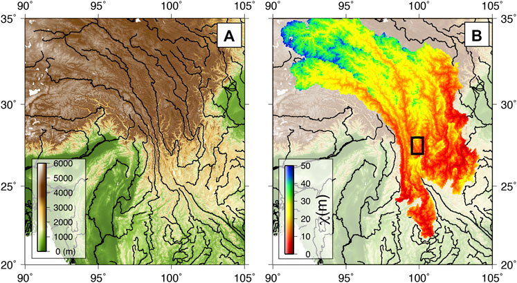
FIGURE 3. The dataset used for the analysis. (A) The HydroSheds hydrologically conditioned topographic dataset with a resolution of ∼90 m (Lehner et al., 2008). (B) Drainage network topology, upstream drainage area and values of were calculated from this dataset with a baselevel set at 500 m for pixels with an upstream drainage area >5 km², with an m value of 0.45, and n value of 1 and a scaling area A₀ of 1 m² after (Yang et al., 2015). The box outlines the extent of Figure 4.

FIGURE 4

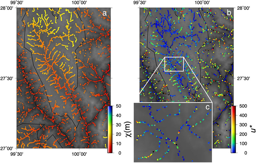
FIGURE 4. 4Subsampling the data. (A) The complete dataset was trimmed by randomly removing 90% of the pixels outside of the low-relief surfaces and 75% within the low-relief surfaces. (B) Local normalized channel steepness maps values highlight regional patterns but are very noisy and thus must be filtered or averaged to make interpretations. (C) Zoomed in portion showing data distribution and variability in the normalized steepness data.

Results

The results are presented as two maps, u* and S.U. and the corresponding misfit value (Figure 5). Here we focus on one result out of several models produced with different values of α and λ. We show the other results in Supplementary Movie S1 and this also provides a means to visualize the sensitivity of the results to the smoothing parameters. In general, small values of the weighting parameters lead to rough models that fit the data well, whereas large weighting parameters produce smoother results that may fit the data poorly (Figure 5A; Supplementary Movie S1). With large values for the weighting parameters, the inversion attempts to minimize the misfit associated with the smoothness constraints (that the Laplacian of the u* values and the S.U. values should be close to zero) resulting in smooth maps. With small values for the weighting parameters, the inversion finds results that fit the data well but are more sensitive to anomalous topography and geomorphic noise, and therefore, results may be meaningless. Within this context, geomorphic noise encapsulates artifacts in the DEM, landslides blocking rivers and over-steepening rivers and small-scale variations in erodibility. It is expected that this noise far exceeds the uncertainty of the DEM (Fox et al., 2015b).

FIGURE 5

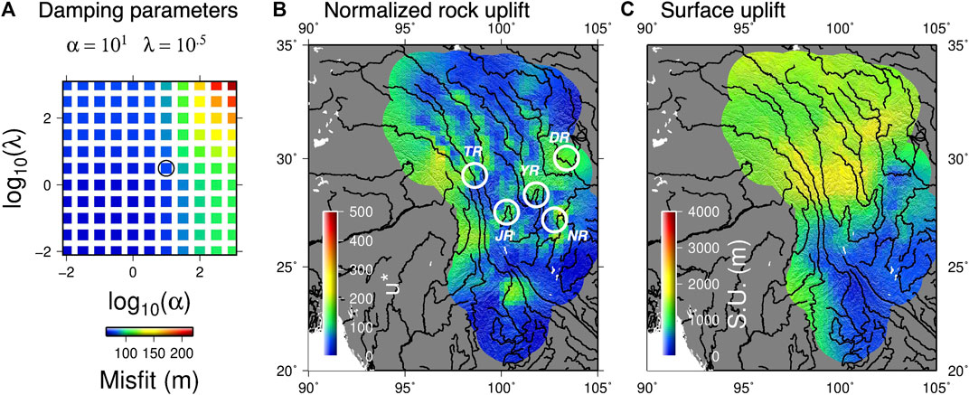
FIGURE 5. Predicted normalized rock uplift rates and spatially variable surface uplift. (A) A two-dimensional L-surface showing the trade-off between model misfit and the two damping parameters which control the roughness of the normalized rock uplift (α) and the surface uplift map (λ). However, each damping parameters influences both maps as the u* and S.U. both predict the topography and control the misfit between the observed and predicted topography, which is minimized by the inversion. A model is preferred that has a small misfit value, but also results in smooth maps. This model is shown by the circle in (A) and the maps are presented in (B) and (C). The sensitivity of the inversion to the damping parameters is presented in Supplementary Movie S1. Low u* values are observed where low-relief surfaces are found but higher values are observed along the trunk streams and the confluence of the Jinsha river with the Niulan River (NR) and aspects of the drainage network, such as large parallel rivers in the Three Rivers area (TR) and the large bends in the Jinsha River (JR), and the Yalong River (YR). High values are also observed close to the Dadu River (DR) which is related to the steep Longmen Shan. These anomalies are more apparent in the rougher models.

In order to choose a preferred model, we employ the same principles behind the L-curve (Hansen, 1992) and search for the damping variables that result in a model with low model roughness and low misfit (i.e., close to the corner of a 2-D L-surface, Richards et al., 2016). A misfit value of approximately 100 m is reasonable: misfit values lower than this suggest that we are fitting noise and misfit values higher than this indicate that the model is not fitting the data. We focus our discussion of the results on features that are robust across a range of values for the damping parameters.

Results show that there are clear short wavelength variations in normalized rock uplift rate and that high values are observed at large confluences and large bends in trunk rivers. By contrast, if the network geometry and values were consistent with a landscape that is being dissected by a wave of incision due to increased rock uplift, a map of relatively uniform u* values less than approximately 200 would be expected. This is because values less than 200 are observed across the low-relief surfaces. We refer to areas with higher than expected u* values as anomalies and these indicate that a topographic surface with low u*, or a low-relief paleotopography, cannot be interpolated between low-relief surfaces and that considerable drainage network reorganization has occurred. In particular, we see high anomalies at the prominent bends in two major tributaries to the Yangtze, the Jinsha and Yalong Rivers, at a confluence with the Niuling River and in the upper reaches within the Dadu (Yang et al., 2020; Suhail et al., 2020) catchment (Figure 5B). The timings of the capture events that formed these anomalies are debated, with the First Bend of the Yangtze either forming in the Eocene (Zheng et al., 2020) or the Pleistocene (Deng et al., 2020). High anomalies also follow these rivers, along with the Lancang, up into Tibet. These anomalies are most pronounced when maps of S.U. are least variable (Supplementary Movie S1) and this is because changes in elevation can be produced with changes in S.U. or changes in u*. Therefore, decreasing changes in S.U. leads to increased variability in u*. A high anomaly is also observed in the Three Gorges area. Crucially, the elevations of the large rivers, where unusual drainage has been previously mapped (Clark et al., 2004), are not used in the inversion. The high normalized channel steepness values that we predict are the result of rivers from low-relief surfaces flowing into the trunk stream at elevations that require anomalously steep trunk river segments. High values are also observed at the eastern end of the Nantinghe Fault (Figure 5B).

Across many of the low-relief surfaces, the residuals are coupled (Figure 6A): large positive values are associated with large negative values, which is caused by drainage divide migration (Fox et al., 2014). Importantly, these residuals highlight that the model is not fitting all channels that are over-steepened and under-steepened by drainage divide migration and capture. To explain all these residuals with the model, the normalized channel steepness map would be even rougher, providing further support for drainage network reorganization.

FIGURE 6

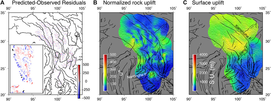
FIGURE 6. Investigating the results of the inversion. (A) The predicted - observed residuals for the low-relief surfaces show that in areas where the misfit is large and positive there are often negative residuals close by. This suggests that drainage divides and river capture are causing pairs of over- and under- steepened $\chi$-elevation relationships. (B) Active faults from GEM database (Styron et al., 2017) compared to the normalized rock uplift map and the surface uplift map (C). Aspects of the results are controlled by active structures, see text for details.

We see evidence that active structures across SE Tibet are influencing our inferred values of S.U. (Figures 6B,C), and this correspondence highlights that short wavelength structures are also contributing to deformation of the low-relief surface. Furthermore, this suggests that damping parameters used in the inversion are not obscuring expected features. In particular, there is a clear change in S.U. across the Lijiang Fault, which is also an area of high strain rates (Copley, 2008; Pan and Shen, 2017; Li et al., 2019). Low values are observed to the east of the Lijiang fault where the Xianschuihe fault splits and to the west of the Lijiang fault, and these areas correspond to areas of GPS-resolved subsidence (Pan and Shen, 2017).

Our predicted elevations can also be displayed along the paths of rivers (Figures 7B,C). This provides an indication of how much incision has occurred at a specific location, if Hypothesis 1 is correct. It is important to point out that here we use incision to indicate the amount of deepening of valleys with respect to the surrounding peaks. In this respect incision is not equal to total erosion. If the erosion rates on the low-relief landscape are assumed to be close to zero, however, this incision is equal to the amount of erosion and could be measured with thermochronometry. The predicted elevations are a function of the pre-incision topography, itself, a result of the $\chi$ distribution and u* values, and the subsequent surface uplift. The predicted elevations follow the low-relief parts of the landscape (cross symbols which appear as solid lines on Figures 7B,C) but plot high above the modern channels in other places. This is because there has been significant rock uplift at these locations and the rivers have incised downwards. Furthermore, there is no requirement that predicted elevations need to decrease with distance downstream as S.U. may be focused at a specific location, warping surfaces upwards. We see that in tributaries of the Yangtze (Figure 7B) the predicted elevations match the low-relief topography relatively well. This also provides insight into how the method works: the low-relief landscapes in river 1 set a regional normalized channel steepness value that is used to project the reconstructed river downstream. Rivers 2 and 3 join river 1 and the information contained in these low-relief surfaces is used to average the normalized channel steepness values. River 4 provides local information on the height of the reconstructed surface and forces the reconstructed surface to remain at high elevations. In reality, there are hundreds of confluences that are simultaneously providing constraints on elevations. In order to match those constraints, variability in u* and/or S.U. is required. These confluences lead to the surface being approximately 1,000 m above the modern river in some locations, predicting 1,000 m of incision. In contrast, for rivers 7, 8, 9, and 10 the maximum predicted incision is approximately 2000 m. The stepped nature of the predicted elevations reflects short wavelength variations in surface uplift and the fact that the rivers may cross the discretized grid in complex ways so that some pixels in the grid may be sampled more than other pixels. A map of predicted incision shows that incision is focused in the Three Gorges region (Figure 8), but does not predict more than approximately 2000 m at any location.

FIGURE 7

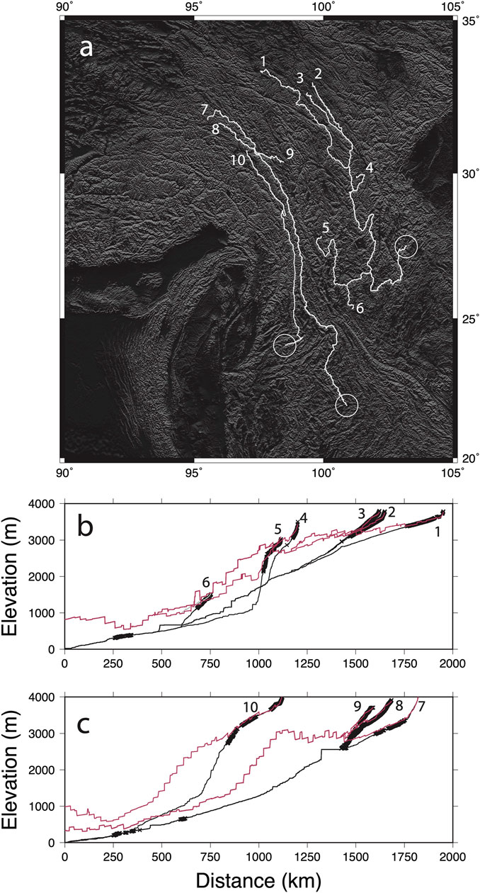
FIGURE 7. Comparison with river profiles. (A) Location map showing the rivers plotted in (B) and (C); (B) River long-profiles extracted from the down sampled DEM, black lines. The crosses are the low-relief nodes used in the inversion, these appear as thick black lines where they are closely spaced. The pink lines are the predicted elevations and account for spatial variability in u* and S.U. and are therefore not monotonic. The stepped nature is due to the fine resolution of the pixels used for the inversion and the fact that the values of u* and S.U. vary over short wavelengths; (C) River long-profiles extracted from Mekong and a tributary of the Salween. Larger amounts of incision are predicted for these rivers.

FIGURE 8

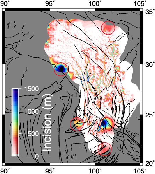
FIGURE 8. Predicted incision. The amount of predicted incision across SE Tibet assuming that the low-relief topographical surface represents a pre-incision landscape. Incision is focused along the rivers in the Three Rivers region, as would be expected from a simple topographic interpolation. Several plotting artifacts are highlighted with red circles and these reflect areas that are unconstrained by the dataset.

Discussion

Temporal Discretization

We have chosen to discretize the tectonic history into two stages. The first stage represents a steady state landscape before the onset of enhanced rock uplift. The second stage represents the cumulative uplift and incision of this landscape and does not make any assumptions about how this varies in time. However, in Hypothesis 1 channel flow would lead to spatial and temporal variations in surface uplift (Clark and Royden, 2000; Schoenbohm et al., 2004). A full inversion of the landscape using river profile modeling with rock uplift rate variable in space and time (Roberts et al., 2012; Fox et al., 2014; Rudge et al., 2015) would require inferring maps of u* at many times in the past. Given that one of our goals is to investigate whether the planform geometry of the drainage network has evolved through time by using a simplified interpolation method, a full inversion that requires assuming this is not justified. Nevertheless, it is important to consider how our simplifications may impact our results. If the areas closest to the plateau were uplifted first, fluvial incision would begin earlier here and there would be less of the paleotopography preserved. Because areas outside of the low-relief surfaces are not used in the analysis, this simply means that we have less data to constrain the surface at these locations.

Effects of Non-Linear Relationships Between Channel Steepness and Erosion Rate

Previous models used to support the conflicting hypotheses, are based on the linear stream power model (i.e., n = 1) and if this underlying model is incorrect then the hypotheses might be slightly different (Goren et al., 2014). We do not attempt to quantify the implications of these underlying assumptions and have adopted the simplified linear stream power model. If n > 1, river segments that are steeper will propagate upstream faster than less steep river segments and vice versa. This would lead to the margins of the low-relief landscape having different $\chi$ values. However, because we only use the elevation data from within the low-relief surfaces to map u* and S.U., the exact $\chi$ value at the edge of the plateau is not significant. Furthermore, the steady state assumption utilized here reduces the dependency on n as variability in n can be mapped into variability in K (Croissant and Braun, 2014).

Cosmogenic-derived catchment averaged erosion rates from across SE Tibet show a non-linear relationship with catchment averaged normalized channel steepness and this suggests that n = 2 (Ouimet et al., 2009). This is based on the assumption that bedrock erodibility is spatially uniform across the study area, that the catchments analyzed are in steady state, and that erosion rates are set by fluvial erosion. Therefore, we explore how increasing the value of n from 1 to 2 would impact our analysis. Royden and Perron (2013), show that the steady state stream power model can be written as

$v^{1/n}=\frac{dh}{d\chi }(7)$

where u* is a simplification of $v$ and $h=z/h_0$ where h₀ is a reference elevation (see Equation 9 of Royden and Perron, 2013). If h₀ is set to 1 m, we can generalize our inversion by treating u* as a dummy variable for (u*)^1/n. Thus we can simply raise our maps of u* by the power of n to get maps of u/(A₀K) for a nonlinear case. If n > 1 spatial variability in the normalized channel steepness values will be amplified, increasing the degree of roughness of the inferred u* map. In contrast if n < 1, variations will be reduced (Figure 9). Future work could leverage this dependency to help constrain the value for n.

FIGURE 9

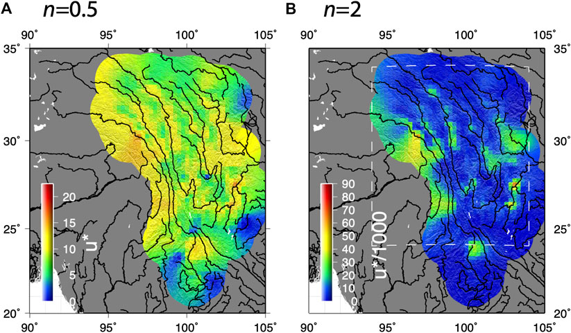
FIGURE 9. Nonlinearities in the stream power model. (A) Normalized channel steepness values for n = 0.5. Overall magnitudes are reduced and there is less spatial variability in the u* map; (B) If n = 2, more spatial variability is predicted, and magnitudes increase. The box shows the regional extent of the map in Figure 10.

In an attempt to determine a value for n for a separate study, Ma et al. (2020) selected the catchment wide erosion rates from Ouimet et al. (2009) for only the Dadu catchment. They found a linear relationship between channel steepness and catchment averaged erosion rates could explain the data. It is unclear whether this is simply because the area analyzed was much smaller or whether slightly different methods were used to calculate normalized channel steepness. Therefore, the value of n for SE Tibet remains debated.

Effects of Spatial Variations in Erodibility

Importantly, we assume that over the scale of SE Tibet there is an effective average erodibility, enabling us to calculate $\chi$ and relate $\chi$ to elevation, and that any erodibility patterns do not correlate with the long wavelength variations in u* or surface uplift. Local studies using a range of methods have determined that the main shape of fluvial long-profiles is not controlled by bedrock lithologies. For example, Kirby et al. (2003) identify spatial variability in erodibility that is limited to local reaches and argue that there is little influence of variable lithology on channel profiles across the Eastern Margin of the Tibetan Plateau. The main knickzone of the middle Mekong River valley is not associated with any variability in lithology (Replumaz et al., 2020). Steep sections of the Dadu River include both sedimentary strata and granites indicating no systematic impact of lithology on river channel steepness (Yang et al., 2020). In the Three Rivers region, Henck et al. (2011) argued that spatial patterns in catchment wide erosion rates are not controlled by spatial variability in lithology. In addition, the elevation and/or preservation of the low-relief surfaces does not correlate with lithology (Clark et al., 2006). From our study, we identify no clear evidence for a correlation between lithology and normalized rock uplift rate and anomalies appear to be associated with river capture events. If the rock uplift rate were uniform across the paleotopography, a steady state had been reached and lithology was responsible for spatial variability in u*, we would expect to see high u* values associated with low K values, and vice versa. Although we see high u* values within an area associated with dense intrusive outcrops (Figure 10A), we also see low values of u* within the lithological boundaries of intrusive igneous rocks, which, to first order, are expected to be the least erodible (Bernard et al., 2019). We also see a wide range in u* values in areas where intrusive rocks are not exposed (Figure 10B). Of course, other lithologies can also be very resistant to erosion, suffice it to say that we do not see a clear correlation between lithology and u* value. Many features of the u* results are relatively long-wavelength features compared to lithological variations. We selected this result to discuss as it represented a good compromise between data fit and smoothness (Supplementary Movie S1). If lithological variations were responsible for the anomalies we detect, this compromise would have led us to select a rougher model. However, even with rougher u* maps (Supplementary Movie S1), there is no clear correlation between lithological variations and u* values. Future work could attempt to assign erodibility values for specific lithologies and recalculate $\chi$, run the inversion, determine how $\chi$ could be modified to smooth the u* maps, update the erodibility values to achieve this $\chi$ distribution and then iterate in this way. However, different lithologies are exposed today compared to when the low-relief landscape was originally formed and this makes this analysis challenging.

FIGURE 10

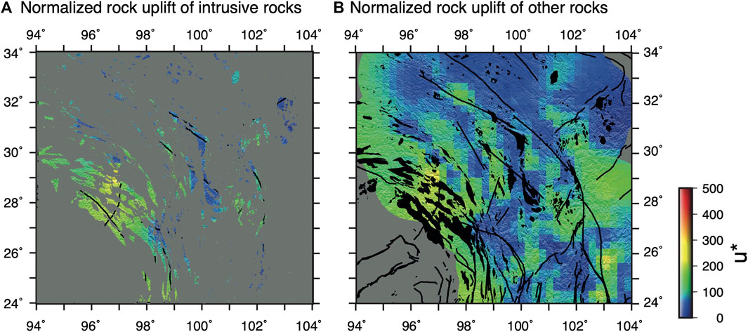
FIGURE 10. The influence of lithology on predicted normalized rock uplift rate. (A) Intrusive rocks colored by the predicted normalized rock uplift rates with the faults included as in Figure 5B. A band of high u* can be seen at approximately 28^oN 97^oW which corresponds to a dense band of intrusive units. However, high and low values of u* are observed across the area; (B) The opposite of Figure 10A showing the predicted normalized rock uplift rates for the other lithologies, with the outcrops of intrusive rocks shown in black. High and low values of u* are observed across both lithological categories and the correlation is not clear. Geological units are simplified after Pan et al. (2004).

It is also important to recognize that other factors may lead to differences between the erodibility of the trunk rivers and the low-relief surfaces, potentially enhancing the development of these low-relief surfaces by increasing K (decreasing our inferred u*), facilitating trunk river incision. For example, the bedload of the large rivers may contain a significant amount of material from hard lithologies from higher up the catchment that would not make up the bedload of the locally drained low-relief surfaces. This would lead to a difference in the contrast between bedrock and bedload in the trunk rivers compared to the low-relief surfaces, and it is this contrast that may lead to local differences in erodibility (Sklar and Dietrich, 2001). In addition, it is clear that the trunk streams flow parallel to major structures, such as suture zones and strike slip faults. It may be expected that these structures would locally increase the erodibility (Roy et al., 2016) and this may facilitate erosion of the trunk rivers and the preservation of the potentially harder low-relief surfaces. Both of these factors may also change through time as different rocks are exhumed leading to changes in bedload or different structures are revealed for rivers to incise into.

We have also assumed that precipitation is uniform in order to relate calculate $\chi$ and relate $\chi$ to elevation. Previous work has accounted for the spatial variability in precipitation to calculate $\chi$ (Yang et al., 2015) however there is also clear evidence that the pattern of precipitation has changed significantly from when the low-relief surface is hypothesized to have been formed to today (Botsyun et al., 2019). Therefore, we have kept precipitation uniform and, in this respect, our study serves as a baseline and factors such as spatially and temporally variable erodibility can be incorporated in future analyses.

Summary

Our approach provides a means to quantitatively assess the continuity of a hypothetical paleo-topography with relatively uniform normalized rock uplift rate. We find that large variability in u* is required if surface uplift is uniform, but that a relatively smooth surface can be found if spatial variability is permitted. However, even with this increased flexibility, anomalously high u* values are found along the main trunk streams. In addition, differences between model-predicted elevations and observed elevations are often positive one side of a drainage divide, but negative on the other side suggesting that these tributaries are out of equilibrium with the regional topography. It should be noted that these residuals only correspond to the low-relief high-elevation parts of the landscape. In order for the u* to be smoother and more uniform, without significantly increasing model misfit, a rougher S.U. map is required, however, this would require short wavelength surface uplift structures, as opposed to a long wavelength mechanism such as lower crustal flow (Clark and Royden, 2000). Ultimately, this choice represents a compromise between roughness and data fit, however, our framework provides a method to ask: what is the relative importance of the two hypotheses? The preferred inversion result (Figure 4) fits almost 75% of the analyzed low-relief nodes to within 100 m, however a model that has smooth u* and S.U. maps, consistent with Hypothesis 1 (α = 10²,λ = 10^1.5) only fits approximately 55% of the data. Therefore, low-relief paleotopography might have existed but the processes required by this model (reduced to its simplest form) only explains about half the data.

While our results lend support to the existence of a low-relief surface that has been uplifted and dissected, this model cannot explain all of the data, and additional factors may have modified erosion rates across the low-relief surfaces, either driven by climatic changes (Zhang et al., 2016; Nie et al., 2018), drainage reorganization (Clark et al., 2004; McPhillips et al., 2016) by drainage divide migration (Yang et al., 2015; Willett, 2017). In addition, the surface is likely to have been deformed by local faulting and lateral movement of low-relief topography as SE Tibet extrudes. However, then the role of a lower crustal low-viscosity channel becomes less clear. What is clear from this analysis is that a topographic surface interpolated between low-relief surfaces found across SE Tibet cannot be used to measure geodynamic processes in time and space. There is limited evidence for low-relief paleotopography in the current topographic data alone and other processes may have entirely shaped modern SE Tibet. Our approach also highlights the limit of utilizing topography alone to interpret landscapes in terms of hypotheses as it is can be an ill-posed inverse problem with multiple scenarios that will lead to indistinguishable features. It is this non-uniqueness that leads to debates about the development of SE Tibet (Yang et al., 2015; Whipple et al., 2017a; Whipple et al., 2017b; Willett, 2017). Future work could use our approach and incorporate diverse datasets and more complexity directly into the analysis. This could include spatially and temporally variable precipitation and erodibility, lateral translation of topography and river networks or hypothesized drainage capture events.

Although our approach provides a means to quantitatively diagnose the continuity of a hypothetical low-relief topographic surface that follows expected slope-area scaling, it does not provide a quantitative test of Hypothesis 1 or 2. In part, this is because the exact smoothness of the two surfaces and degree of data misfit required for Hypothesis 1 have not been specified in the literature. Our approach incorporates the strengths of the different approaches used to extract information from river networks, outlined in Using Fluvial Metrics to Test the Hypotheses, but adds additional flexibility. Furthermore, because we are not extracting individual channels from the DEM our approach potentially uses more of the data and we are not selecting which channels to highlight. In order to really understand the topographic development of SE Tibet, data that resolve temporal changes in erosion through time at the scale of individual patches of low-relief topography are required. Thermochronology would be the ideal tool to measure the exhumation rate history across the low-relief landscapes and the surrounding canyons (Gourbet et al., 2020) however, the amount of relief change is right at the limits of the method (Braun, 2002). What is clear from thermochronology is that exhumation rates have been highly variable in space and time, with the amount of exhumation at some locations being far greater than the amount predicted from valley incision alone (Zhang et al., 2016; Cook et al., 2018; Liu-Zeng et al., 2018; Ge et al., 2020; Replumaz et al., 2020). If this exhumation is associated with local high rates of rock uplift, and if the erosion rates on the surrounding low-relief surfaces remain low, large amounts of S.U. would be observed leading to obvious discontinuities in the low-relief surface. These have not been observed and thus this highlights the importance of processes that create low-relief surfaces in situ, supporting Hypothesis 2.

In order to falsify Hypothesis 2, future work could search for an absence of low-relief landscapes at intermediate elevations. This is challenging however as Hypothesis 2 predicts that landscapes that have lost upstream drainage area progressively lose relief and are thus most prominent at the highest elevations. Furthermore, the landscape is developing in an area of active deformation. This means that tectonics may respond to changes in surface topography in such a way that sets a limit on how high the low-relief landscapes can be uplifted. This would mean that all the low-relief landscapes might attain coherent, gradually varying, elevations set by the strength of the crust and faults. If only the elevations of the low-relief surfaces were used, this would support Hypothesis 1. We have not mapped low-relief surfaces across SE Tibet and have used published surfaces for our analysis (Clark et al., 2004), however, there does appear to be low-relief landscapes at intermediate elevations across the Upper Yangtze River (Liu et al., 2019). Alternatively, in situ erosion rate histories within the low-relief landscapes could be measured using low-temperature thermochronometry. The fingerprint of Hypothesis 2 would be decreases in exhumation rate associated with area loss coupled with increases in exhumation in surrounding canyons.

Data Availability Statement

Publicly available datasets were analyzed in this study. This data can be found here: https://www.hydrosheds.org.

Author Contributions

All authors contributed to the design, analysis, and writing of the manuscript.

Conflict of Interest

The authors declare that the research was conducted in the absence of any commercial or financial relationships that could be construed as a potential conflict of interest.

Acknowledgments

We thank G. Hilley, J. P. Avouac and two reviewers for providing helpful feedback and S. D. Willett for stimulating discussions. This study was supported by NERC (NE/N015479/1).

Supplementary Material

The Supplementary Material for this article can be found online at: https://www.frontiersin.org/articles/10.3389/feart.2020.587597/full#supplementary-material

References

Bernard, T., Sinclair, H. D., Gailleton, B., Mudd, S. M., and Ford, M. (2019). Lithological control on the post-orogenic topography and erosion history of the Pyrenees. Earth Planet Sci. Lett. 518, 53–66. doi:10.1016/j.epsl.2019.04.034

CrossRef Full Text | Google Scholar

Botsyun, S., Sepulchre, P., Donnadieu, Y., Risi, C., Licht, A., and Rugenstein, J. K. C. (2019). Revised paleoaltimetry data show low Tibetan Plateau elevation during the Eocene. Science 363 (6430), eaaq1436. doi:10.1126/science.aaq1436

CrossRef Full Text | Google Scholar

Braun, J. (2002). Quantifying the effect of recent relief changes on age–elevation relationships. Earth Planet Sci. Lett. 200 (3–4), 331–343. doi:10.1016/s0012-821x(02)00638-6

CrossRef Full Text | Google Scholar

Clark, M. K., and Royden, L. H. (2000). Topographic ooze: building the eastern margin of Tibet by lower crustal flow. Geology 28, 703–706. doi:10.1130/0091-7613(2000)28<703:tobtem>2.0.co;2

CrossRef Full Text | Google Scholar

Clark, M. K., Royden, L. H., Whipple, K. X., Burch el, B. C., Zhang, X., and Tang, W. (2006). Use of a regional, relict landscape to measure vertical deformation of the eastern Tibetan Plateau. J. Geophys. Res. Earth Surface 111, 187-10. doi:10.1029/2005jf000294

CrossRef Full Text | Google Scholar

Clark, M. K., Schoenbohm, L. M., Royden, L. H., Whipple, K. X., Burchfiel, B. C., Zhang, X., et al. (2004). Surface uplift, tectonics, and erosion of eastern Tibet from large-scale drainage patterns. Tectonics 23 (1). doi:10.1029/2002tc001402

CrossRef Full Text | Google Scholar

Cook, K. L., Hovius, N., Wittmann, H., Heimsath, A. M., and Lee, Y.-H. (2018). Causes of rapid uplift and exceptional topography of Gongga Shan on the eastern margin of the Tibetan Plateau. Earth Planet Sci. Lett. 481, 328–337. doi:10.1016/j.epsl.2017.10.043

CrossRef Full Text | Google Scholar

Copley, A. (2008). Kinematics and dynamics of the southeastern margin of the Tibetan Plateau. Geophys. J. Int. 174, 1081–1100. doi:10.1111/j.1365-246x.2008.03853.x

CrossRef Full Text | Google Scholar

Croissant, T., and Braun, J., (2014). Constraining the stream power law: a novel approach combining a landscape evolution model and an inversion method. Earth Surf. Dynam. Discuss. 2 (1), 155–166. doi:10.5194/esurf-2-155-2014

CrossRef Full Text | Google Scholar

Deng, B., Chew, D., Mark, C., Liu, S., Cogné, N., Jiang, L., et al. (2020). Late Cenozoic drainage reorganization of the paleo-Yangtze river constrained by multi-proxy provenance analysis of the Paleo-lake Xigeda. Geol. Soc. Am. Bull. doi:10.1130/b35579.1

CrossRef Full Text | Google Scholar

Egholm, D. L., Jansen, J. D., Brædstrup, C. F., Pedersen, V. K., Andersen, J. L., Ugelvig, S. V., et al. (2017). Formation of plateau landscapes on glaciated continental margins. Nat. Geosci. 10 (8), 592. doi:10.1038/ngeo2980

CrossRef Full Text | Google Scholar

Egholm, D. L., Nielsen, S. B., Pedersen, V. K., and Lesemann, J.-E. (2009). Glacial effects limiting mountain height. Nature 460 (7257), 884. doi:10.1038/nature08263

CrossRef Full Text | Google Scholar

England, P., and Molnar, P., (1990). Surface uplift, uplift of rocks, and exhumation of rocks. Geology 18 (12), 1173–1177. doi:10.1130/0091-7613(1990)018<1173:suuora>2.3.co;2

CrossRef Full Text | Google Scholar

Ferrier, K. L., Huppert, K. L., and Perron, J. T. (2013). Climatic control of bedrock river incision. Nature 496, 206–209. doi:10.1038/nature11982

CrossRef Full Text | Google Scholar

Fox, M. (2019). A linear inverse method to reconstruct paleo-topography. Geomorphology 337, 151–164. doi:10.1016/j.geomorph.2019.03.034

CrossRef Full Text | Google Scholar

Fox, M., Bodin, T., and Shuster, D. L. (2015b). Abrupt changes in the rate of Andean Plateau uplift from reversible jump Markov chain Monte Carlo inversion of river profiles. Geomorphology 238, 1–14. doi:10.1016/j.geomorph.2015.02.022

CrossRef Full Text | Google Scholar

Fox, M., Herman, F., Kissling, E., and Willett, S. D. (2015a). Rapid exhumation in the Western Alps driven by slab detachment and glacial erosion. Geology 43 (5), 379–382. doi:10.1130/g36411.1

CrossRef Full Text | Google Scholar

Fox, M., Goren, L., May, D. A., and Willett, S. D. (2014). Inversion of fluvial channels for paleorock uplift rates in Taiwan. J. Geophys. Res. Earth Surf. 119 (9), 1853–1875. doi:10.1002/2014jf003196

CrossRef Full Text | Google Scholar

Ge, Y., Liu-Zeng, J., Zhang, J., Wang, W., Tian, Y., Fox, M., et al. (2020). Spatio-temporal variation in rock exhumation linked to large-scale shear zones in the southeastern Tibetan Plateau. Sci. China Earth Sci. 63, 512–532. doi:110.1007/s11430-019-9567-y

CrossRef Full Text | Google Scholar

Goren, L., Fox, M., and Willett, S. D. (2014). Tectonics from fluvial topography using formal linear inversion: theory and applications to the Inyo Mountains, California. J. Geophys. Res. Earth Surf. 119, 1651–1681. doi:10.1002/2014jf003079

CrossRef Full Text | Google Scholar

Gourbet, L., Yang, R., Fellin, M. G., Paquette, J.-L., Willett, S. D., Gong, J., et al. (2020). Evolution of the Yangtze river network, southeastern Tibet: insights from thermochronology and sedimentology. Lithosphere 12 (1), 3–18. doi:10.1130/l1104.1

CrossRef Full Text | Google Scholar

Hales, T. C., and Roering, J. J. (2007). Climatic controls on frost cracking and implications for the evolution of bedrock landscapes. J. Geophys. Res. Earth Surf. 112 (F2). doi:10.1029/2006jf000616

CrossRef Full Text | Google Scholar

Hallet, B., and Molnar, P. (2001). Distorted drainage basins as markers of crustal strain east of the Himalaya. J. Geophys. Res. 106 (B7), 13697–13709. doi:10.1029/2000jb900335

CrossRef Full Text | Google Scholar

Hansen, P. C. (1992). Analysis of discrete ill-posed problems by means of the L-curve. SIAM Rev. 34, 561–580. doi:10.1137/1034115

CrossRef Full Text | Google Scholar

Henck, A. C., Huntington, K. W., Stone, J. O., Montgomery, D. R., and Hallet, B. (2011). Spatial controls on erosion in the three rivers region, southeastern Tibet and southwestern China. Earth Planet Sci. Lett. 303 (1-2), 71–83. doi:10.1016/j.epsl.2010.12.038

CrossRef Full Text | Google Scholar

Howard, A. D. (1994). A detachment-limited model of drainage basin evolution. Water Resour. Res. 30, 2261–2285. doi:10.1029/94wr00757

CrossRef Full Text | Google Scholar

Kirby, E., and Whipple, K. X. (2012). Expression of active tectonics in erosional landscapes. J. Struct. Geol. 44, 54–75. doi:10.1016/j.jsg.2012.07.009

CrossRef Full Text | Google Scholar

Kirby, E., Whipple, K. X., Tang, W., and Chen, Z. (2003). Distribution of active rock uplift along the eastern margin of the Tibetan Plateau: inferences from bedrock channel longitudinal profiles. J. Geophys. Res. Solid Earth 108 (B4), 2217. doi:10.1029/2001jb000861

CrossRef Full Text | Google Scholar

Lehner, B., Verdin, K., and Jarvis, A. (2008). New global hydrography derived from spaceborne elevation data. Eos Trans. AGU 89 (10), 93–94. doi:10.1029/2008eo100001

CrossRef Full Text | Google Scholar

Li, Y., Liu, M., Li, Y., and Chen, L. (2019). Active crustal deformation in southeastern Tibetan Plateau: the kinematics and dynamics. Earth Planet Sci. Lett. 523, 115708. doi:10.1016/j.epsl.2019.07.010

CrossRef Full Text | Google Scholar

Liu, F., Gao, H., Pan, B., Li, Z., and Su, H. (2019). Quantitative analysis of planation surfaces of the upper Yangtze River in the Sichuan-yunnan region, Southwest China. Front. Earth Sci. 13 (1), 55–74. doi:10.1007/s11707-018-0707-y

CrossRef Full Text | Google Scholar

Liu-Zeng, J., Zhang, J., McPhillips, D., Reiners, P., Wang, W., Pik, R., et al. (2018). Multiple episodes of fast exhumation since Cretaceous in southeast Tibet, revealed by low-temperature thermochronology. Earth Planet Sci. Lett. 490, 62–76. doi:10.1016/j.epsl.2018.03.011

CrossRef Full Text | Google Scholar

Ma, Z., Zhang, H., Wang, Y., Tao, Y., and Li, X. (2020). Inversion of Dadu River bedrock channels for the late cenozoic uplift history of the eastern Tibetan Plateau. Geophys. Res. Lett.

Google Scholar

McPhillips, D., Hoke, G. D., Liu-Zeng, J., Bierman, P. R., Rood, D. H., and Niedermann, S. (2016). Dating the incision of the Yangtze River gorge at the First Bend using three-nuclide burial ages. Geophys. Res. Lett. 43 (1), 101–110. doi:10.1002/2015gl066780

CrossRef Full Text | Google Scholar

Molnar, P., Boos, W. R., and Battisti, D. S. (2010). Orographic controls on climate and paleoclimate of Asia: thermal and mechanical roles for the Tibetan Plateau. Annu. Rev. Earth Planet Sci. 38, 77–102. doi:10.1146/annurev-earth-040809-152456

CrossRef Full Text | Google Scholar

Mudd, S. M., Attal, M., Milodowski, D. T., Grieve, S. W. D., and Valters, D. A. (2014). A statistical framework to quantify spatial variation in channel gradients using the integral method of channel profile analysis. J. Geophys. Res. Earth Surf. 119, 138–152. doi:10.1002/2013jf002981

CrossRef Full Text | Google Scholar

Mudd, S. M., Clubb, F. J., Gailleton, B., and Hurst, M. D. (2018). How concave are river channels? Earth Surf. Dynam. Discuss. 6 (2), 505–523. doi:10.5194/esurf-6-505-2018

CrossRef Full Text | Google Scholar

Nie, J., Ruetenik, G., Gallagher, K., Hoke, G., Garzione, C. N., Wang, W., et al. (2018). Rapid incision of the Mekong River in the middle Miocene linked to monsoonal precipitation. Nat. Geosci. 11, 944–948. doi:10.1038/s41561-018-0244-z

CrossRef Full Text | Google Scholar

Ouimet, W. B., Whipple, K. X., and Granger, D. E. (2009). Beyond threshold hillslopes: channel adjustment to base-level fall in tectonically active mountain ranges. Geology 37 (7), 579–582. doi:10.1130/g30013a.1

CrossRef Full Text | Google Scholar

Ouimet, W., Whipple, K., Royden, L., Reiners, P., Hodges, K., and Pringle, M. (2010). Regional incision of the eastern margin of the Tibetan Plateau. Lithosphere 2, 50–63. doi:10.1130/l57.1

CrossRef Full Text | Google Scholar

Pan, G. T., Ding, J., Yao, D. S., and Wang, L. Q. (2004). Guidebook of 1: 1,500,000 geologic map of the Qinghai–Xizang (Tibet) plateau and adjacent areas. Chengdu, China: Chengdu Cartographic Publishing House, 48.

Google Scholar

Pan, Y., and Shen, W. B. (2017). Contemporary crustal movement of southeastern Tibet: constraints from dense GPS measurements. Sci. Rep. 7, 45348. doi:10.1038/srep45348

CrossRef Full Text | Google Scholar

Perron, J. T., and Royden, L. (2012). An integral approach to bedrock river profile analysis. Earth Surf. Process. Landf. 38, 570–576. doi:10.1002/esp.3302

CrossRef Full Text | Google Scholar

Replumaz, A., San José, M., Margirier, A., van der Beek, P., Gautheron, C., Leloup, P. H., et al. (2020). Tectonic control on rapid late Miocene—quaternary incision of the Mekong River Knickzone, southeast Tibetan Plateau. Tectonics 39 (2), e2019TC005782. doi:10.1029/2019tc005782

CrossRef Full Text | Google Scholar

Richards, F. D., Hoggard, M. J., and White, N. J. (2016). Cenozoic epeirogeny of the Indian peninsula. Geochem. Geophys. Geosyst. 17, 4920–4954. doi:10.1002/2016gc006545

CrossRef Full Text | Google Scholar

Roering, J. J., Marshall, J., Booth, A. M., Mort, M., and Jin, Q. (2010). Evidence for biotic controls on topography and soil production. Earth Planet Sci. Lett. 298 (1-2), 183–190. doi:10.1016/j.epsl.2010.07.040

CrossRef Full Text | Google Scholar

Roberts, G. G., Paul, J. D., White, N., and Winterbourne, J. (2012). Temporal and spatial evolution of dynamic support from river profiles: a framework for Madagascar. Geochem. Geophys. Geosyst. 13 (4), 1087. doi:10.1029/2012gc004040

CrossRef Full Text | Google Scholar

Roy, S. G., Tucker, G. E., Koons, P. O., Smith, S. M., and Upton, P. (2016). A fault runs through it: modeling the influence of rock strength and grain-size distribution in a fault-damaged landscape. J. Geophys. Res. Earth Surf. 121 (10), 1911–1930. doi:10.1002/2015jf003662

CrossRef Full Text | Google Scholar

Royden, L., and Taylor Perron, J. (2013). Solutions of the stream power equation and application to the evolution of river longitudinal profiles. J. Geophys. Res.: Earth Surface 118 (2), 497–518

Rudge, J. F., Roberts, G. G., White, N. J., and Richardson, C. N. (2015). Uplift histories of Africa and Australia from linear inverse modeling of drainage inventories. J. Geophys. Res. Earth Surf. 120 (5), 894–914. doi:10.1002/2014jf003297

CrossRef Full Text | Google Scholar

Schaller, M., Ehlers, T. A., Lang, K. A. H., Schmid, M., and Fuentes-Espoz, J. P. (2018). Addressing the contribution of climate and vegetation cover on hillslope denudation, Chilean Coastal Cordillera (26°-38°S). Earth Planet Sci. Lett. 489, 111–122. doi:10.1016/j.epsl.2018.02.026

CrossRef Full Text | Google Scholar

Scherler, D., DiBiase, R. A., Fisher, G. B., and Avouac, J.-P. (2017). Testing monsoonal controls on bedrock river incision in the Himalaya and Eastern Tibet with a stochastic-threshold stream power model. J. Geophys. Res. Earth Surf. 122 (7), 1389–1429. doi:10.1002/2016jf004011

CrossRef Full Text | Google Scholar

Schoenbohm, L. M., Whipple, K. X., Burchfiel, B. C., and Chen, L. (2004). Geomorphic constraints on surface uplift, exhumation, and plateau growth in the Red River region, Yunnan Province, China. Geol. Soc. Am. Bull. 116, 895–909. doi:10.1130/b25364.1

CrossRef Full Text | Google Scholar

Schwanghart, W., and Scherler, D. (2020). Divide mobility controls knickpoint migration on the Roan Plateau (Colorado, USA). Geology 48, 698–702. 10.1130/G47054.1

CrossRef Full Text | Google Scholar

Sklar, L. S., and Dietrich, W. E., (2001). Sediment and rock strength controls on river incision into bedrock. Geology 29 (12), 1087–1090. doi:10.1130/0091-7613(2001)029<1087:sarsco>2.0.co;2

CrossRef Full Text | Google Scholar

Sternai, P., Herman, F., Champagnac, J.-D., Fox, M., Salcher, B., and Willett, S. D. (2012). Pre-glacial topography of the European Alps. Geology 40, 1067–1070. doi:10.1130/g33540.1

CrossRef Full Text | Google Scholar

Styron, R. H., Garcia, J., and Pagani, M. (2017). “The GEM Global Active Faults Database: the growth and synthesis of a worldwide database of active structures for PSHA, research, and education,” in AGU fall meeting abstracts, Washington, DC, December 11–15, 2017.

Google Scholar

Suhail, H. A., Yang, R., Chen, H., and Rao, G. (2020). The impact of river capture on the landscape development of the Dadu River drainage basin, eastern Tibetan Plateau. J. Asian Earth Sci. 198, 104377. doi:10.1016/j.jseaes.2020.104377

CrossRef Full Text | Google Scholar

Tan, X., Liu, Y., Lee, Y.-H., Lu, R., Xu, X., Suppe, J., et al. (2019). Parallelism between the maximum exhumation belt and the Moho ramp along the eastern Tibetan Plateau margin: coincidence or consequence? Earth Planet Sci. Lett. 507, 73–84. doi:10.1016/j.epsl.2018.12.001

CrossRef Full Text | Google Scholar

Tapponnier, P., Peltzer, G. L. D. A. Y., Le Dain, A. Y., Armijo, R., and Cobbold, P. (1982). Propagating extrusion tectonics in Asia: new insights from simple experiments with plasticine. Geology 10 (12), 611–616. doi:10.1130/0091-7613(1982)10<611:petian>2.0.co;2

CrossRef Full Text | Google Scholar

Whipple, K. X., DiBiase, R. A., Ouimet, W. B., and Forte, A. M. (2017a). Preservation or piracy: diagnosing low-relief, high-elevation surface formation mechanisms. Geology 45, 91–94. doi:10.1130/g38490.1

CrossRef Full Text | Google Scholar

Whipple, K. X., DiBiase, R. A., Ouimet, W. B., and Forte, A. M. (2017b). Preservation or piracy: diagnosing low-relief, high-elevation surface formation mechanisms: reply. Geology 45, e422. doi:10.1130/g39252y.1

CrossRef Full Text | Google Scholar

Whipple, K. X., Forte, A. M., DiBiase, R. A., Gasparini, N. M., and Ouimet, W. B. (2017c). Timescales of landscape response to divide migration and drainage capture: implications for the role of divide mobility in landscape evolution. J. Geophys. Res. Earth Surf. 122 (1), 248–273. doi:10.1002/2016jf003973

CrossRef Full Text | Google Scholar

Willett, S. D. (2017). Preservation or piracy: diagnosing low-relief, high-elevation surface formation mechanisms: comment. Geology 45, e421. doi:10.1130/g38929c.1

CrossRef Full Text | Google Scholar

Willett, S. D., McCoy, S. W., Perron, J. T., Goren, L., and Chen, C. Y. (2014). Dynamic reorganization of river basins. Science 343. 1248765. doi:10.1126/science.1248765

CrossRef Full Text | Google Scholar

Yang, R., Suhail, H. A., Gourbet, L., Willett, S. D., Fellin, M. G., Lin, X., et al. (2020). Early Pleistocene drainage pattern changes in Eastern Tibet: constraints from provenance analysis, thermochronometry, and numerical modeling. Earth Planet Sci. Lett. 531, 115955. doi:10.1016/j.epsl.2019.115955

CrossRef Full Text | Google Scholar

Yang, R., Willett, S. D., and Goren, L. (2015). In situ low-relief landscape formation as a result of river network disruption. Nature 520, 526–529. doi:10.1038/nature14354

CrossRef Full Text | Google Scholar

Zhang, H., Oskin, M. E., Liu-Zeng, J., Zhang, P., Reiners, P. W., and Xiao, P. (2016). Pulsed exhumation of interior eastern Tibet: implications for relief generation mechanisms and the origin of high-elevation planation surfaces. Earth Planet Sci. Lett. 449, 176–185. doi:10.1016/j.epsl.2016.05.048

CrossRef Full Text | Google Scholar

Zheng, H., Clift, P. D., He, M., Bian, Z., Liu, G., Liu, X., et al. (2020). Formation of the first bend in the late Eocene gave birth to the modern Yangtze River, China. Geology 48. 10.1130/G48149.1

CrossRef Full Text | Google Scholar