 Chan Yeong Kim
 Soonyoung Yu
 Yun-Yeong Oh2†
- 1Korea Institute of Geoscience and Mineral Resources (KIGAM), Daejeon, South Korea
- 2Department of Earth and Environmental Sciences and Korea-CO2 Storage Environmental Management (K-COSEM) Research Center, Korea University, Seoul, South Korea
Temporal changes of soil CO2 flux (FCO2) and soil CO2 concentration ([CO2]v) were surveyed in a natural CO2 emission site to characterize the factors controlling the short-term temporal variation of geogenic FCO2 in a non-volcanic and seismically inactive area. Due to a lack of long-term monitoring system, FCO2 was discontinuously measured for three periods: Ⅰ, Ⅱ at a high FCO2 point (M17) and Ⅲ about 30 cm away. Whereas [CO2]v was investigated at a point (60 cm depth) for all periods. A 2.1 magnitude earthquake occurred 7.8 km away and 20 km deep approximately 12 h before the period Ⅱ. The negative correlation of FCO2 with air pressure suggested the non-negligible advective transport of soil CO2. However, FCO2 was significantly and positively related with air temperature as well, and [CO2]v showed different temporal changes from FCO2. These results indicate the diffusive transport of soil CO2 dominant in the vadose zone, while the advection near the surface. Meanwhile [CO2]v rapidly decreased while an anomalous FCO2 peak was observed during the period Ⅱ, and the CO2 emission enhanced by the earthquake was discussed as a possible reason for the synchronous decrease in [CO2]v and increase in FCO2. In contrast, [CO2]v increased to 56.8% during the period Ⅲ probably due to low gas diffusion at cold weather. In addition, FCO2 was low during the period Ⅲ and showed different correlations with measurements compared to FCO2 at M17, implying heterogeneous CO2 transport conditions at the centimeter scale. The abnormal FCO2 observed after the earthquake in a seismically inactive area implies that the global natural CO2 emission may be higher than the previous estimation. The study result suggests a permanent FCO2 monitoring station in tectonically stable regions to confirm the impact of geogenic CO2 to climate change and its relation with earthquakes.
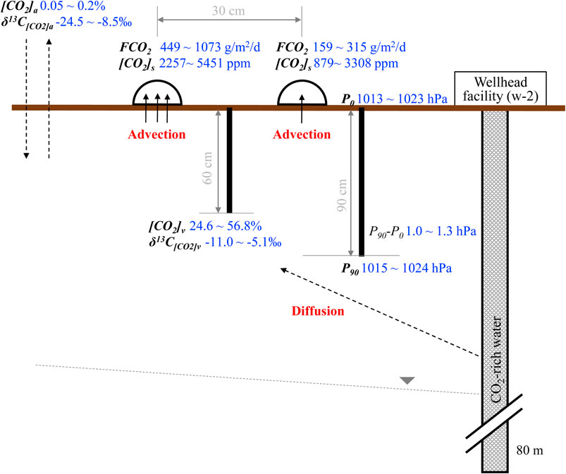
GRAPHICAL ABSTRACT
Introduction
Annual CO2 emission from the Earth was estimated to be approximately 600 million tonnes, with almost half produced from subaerial volcanism and the other half from non-volcanic inorganic degassing such as tectonic activities (Kerrick et al., 1995; Mörner and Etiope, 2002; Chiodini et al., 2005; Burton et al., 2013; Fischer et al., 2019). Lots of studies have been performed on the spatial distributions of geogenic soil CO2 flux (FCO2) for various purposes: to identify the extent of anomalous CO2 outflow and its relation to the structural geology (e.g., Annunziatellis et al., 2008; Ciotoli et al., 2014; Ciotoli et al., 2016; Jung et al., 2014; Ascione et al., 2018; Kim et al., 2019); to calculate the total CO2 output (e.g., Chiodini et al., 1999; Cardellini et al., 2003; Sun et al., 2018); to investigate the origin of CO2 (e.g., Schroder et al., 2016; Chen et al., 2020); to assess volcanic (e.g., Chiodini et al., 2001; Hernández et al., 2001; Carapezza et al., 2011; Morita et al., 2019) and seismic hazards (eg, Camarda et al., 2016; Fischer et al., 2017; Sciarra et al., 2017).
Meanwhile, the temporal changes of geogenic FCO2 and their controlling factors were relatively less studied and mostly in volcanic or seismic areas (e.g., Chiodini et al., 1998; Granieri et al., 2003; Carapezza et al., 2011; Camarda et al., 2016; Camarda et al., 2019; Oliveira et al., 2018; Morita et al., 2019; Chen et al., 2020). Morita et al. (2019) showed that barometric pressure, air temperature, soil temperature and humidity, and wind speed were decisive variables that could explain more than half of the variations in FCO2 at 1 km southwest of the active crater of Aso volcano, while the residuals were explained using an increase in magmatic CO2 flux. Repeated measurements by Chiodini et al. (1998) showed that FCO2 was governed by the change in barometric pressure, while other meteorological parameters such as rain, soil and air temperature, and humidity also influenced FCO2 in volcanic and geothermal areas. As for seismically active regions, Kerrick and Caldeira (1993), Kerrick and Caldeira (1994), Kerrick and Caldeira (1998), and Kerrick et al. (1995) studied metamorphic CO2 degassing, including convective hydrothermal CO2 emission. In addition, Chiodini et al. (1999) suggested the non-volcanic CO2 derived from mantle degassing and/or metamorphic decarbonation in Central Italy. Lee et al. (2016) estimated 4 Mt/yr of mantle-derived CO2 released along deep faults in the Magadi–Natron Basin at the border between Kenya and Tanzania. Ascione et al. (2018) introduced anomalously high FCO2 resulting from the combination of 1) intense CO2 generation from magmatic bodies causing decarbonation of carbonate rocks; 2) a very thin or absent top seal overlying the carbonate reservoirs; 3) the occurrence of a dense network of active fault segments at the tip of a major crustal fault zone.
Moreover, seismic activity has been considered as an endogenous cause of the temporal variation of geogenic FCO2 (Camarda et al., 2016; Camarda et al., 2019; Fischer et al., 2017; Sciarra et al., 2017; Chen et al., 2020). Specifically, Camarda et al. (2019) found that, of the two anomalous FCO2 periods (A and C), the period A had a seismic swarm (3,471 seismic events in 79 days; Ricci et al., 2015) and thus showed the higher-amplitude anomalies than the period C. Camarda et al. (2016) showed the high spatial and temporal correlation between seismicity and FCO2 in a district with continuous seismic activity, whereas FCO2 varied independently in the districts with low and sporadic seismicity. According to Chen et al. (2020), seismic activity also can be responsible for the jumpily temporal variations of CO2 concentration and flux in soil gas wells. Furthermore, vibro-stimulation was applied to increase the oil production based on the physics that the rate of degassing increases due to vibration energy (Kouznetsov et al., 1998; Kouznetsov et al., 2002).
However, studies have been rarely conducted about either the temporal variation of geogenic FCO2 or the effect of small seismic events to FCO2 in a geologically quiescent (e.g., non-volcanic or seismically inactive) environment. As an alternative, CO2-rich waters have been studied in tectonically stable regions, in particular as a natural analogue study of geologic carbon storage to understand CO2 leakage (e.g., Chae et al., 2016), because non-volcanic CO2 is discharged by high-CO2 groundwater as well as by focused degassing (Chiodini et al., 1999). For instance, in South Korea, which has no active volcanoes and had been relatively safe from seismic activity until the 2016 Gyeongju earthquake (M 5.8) (Woo et al., 2019), CO2-rich waters have been studied to identify anomalously high soil CO2 areas, and their origins (e.g., magmatic degassing, metamorphic devolatilization, oxidation of organic matter) and ascending pathways. According to Jeong et al. (2005), the CO2 gas derived from a deep-seated source moves into the groundwater system along faults or geologic boundaries in South Korea. However, FCO2 has been rarely studied, which motivated this study.
This study aimed 1) to characterize the temporal variation of FCO2 in a non-volcanic and seismically inactive site (Figure 1A) where soil CO2 was suggested to have a deep-seated magmatic origin (Kim et al., 2019), and 2) to identify the factors controlling the temporal changes of geogenic FCO2. The time-variant CO2 supply and the effect of a small earthquake were discussed. This study contributes to provide a new study direction of long-term FCO2 monitoring to the atmosphere in tectonically stable regions, which is important to assess due to the impacts of CO2 on climate change, whereas many existing studies have focused on volcanic or seismic regions.
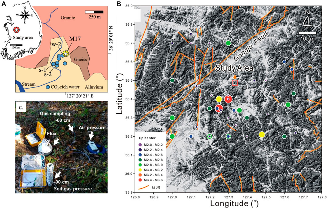
FIGURE 1. Study area. (A) Location of the study point (M17) on the geological map. Five CO2-rich groundwater wells including w-2 and two springs (s-1 and s-2) are also shown. (B) 49 epicenters around the study area in the past 30 years (KMA, 2019) including a recent earthquake (magnitude 2.1 and 20 km depth) occurring on November 19, 2018 at 7.8 km southwest of the study area. The larger circle indicates the larger magnitude. (C) Field measurements.
Study Area
The study area (Daepyeong; Lat. 36o29′01″N and Long. 127o20′21″E) is located in the central South Korea (Figure 1A) and in the middle of a small basin (about 1.1 km2). The small watershed is surrounded by mountains lower than 270 m above sea level, and the low and flat area of the basin is mostly used for rice cultivation. There are also farmhouses and gardens that cultivate vegetables, fruits, and pine saplings on a small scale.
The bedrock of the study area consists of Precambrian gneiss that was intruded by Jurassic granite (Figure 1A). The gneiss and granite are overlain by Quaternary sediments at lower altitudes. It is noticeable that the study area is located at the geologic boundary between gneiss and granite, along which five CO2-rich groundwater wells and two CO2-rich springs occur (Figure 1A; Jeong et al., 2001; Jeong et al., 2005; Chae et al., 2016). Chae et al. (2016) observed fractures (fissures and/or joints) and CO2 bubbles from the fractures at a CO2-rich spring (s-1). Kim et al. (2019) found a high FCO2 point (M17 in Figure 1A) about 1.8 m away from a CO2-rich groundwater well (w-2) to release geogenic CO2 through the soil layer among a total of 94 points within 1 km2. The well (w-2) has a depth of 80 m and a diameter of 150 mm, and CO2-rich water is irregularly taken at w-2 for domestic usage by countless residents. The contact of gneiss and granite is observed on a slope near the well w-2.
A fault has not been identified in the study area (MCT et al., 2006), whereas there are faults in a regional scale including the closest Gongju Fault approximately 13 km away from the study area (Figure 1B). At the regional scale, the study area is located on the southwest of the NE/SW trending Ogcheon Belt (Ogcheon region). The Ogcheon Belt is a fold-and-thrust belt affected by several deformational phases, and the Ogcheon region is mainly composed of metamorphosed clastic and volcanic rocks (Kihm and Kim, 2003). In the Ogcheon region, CO2-rich waters occur in the NE-SW direction (Supplementary Figure S1), parallel to the Gongju Fault and Ogcheon Belt, which implies the relation of CO2-rich waters to faults or fractures, while no evidence has yet been found.
A total of 49 small earthquakes (≥magnitude 2.0) occurred within 30 km from the study area in the past 30 years (Figure 1B; KMA, 2019), including the 2.1 magnitude (M) earthquake occurring on 03:34 November 19, 2018 at 7.8 km southwest of the study area and 20 km deep. The information of focal depths is available only for five earthquakes occurring after 2017 and in the range of 11–20 km. The distribution of earthquake epicenters and their magnitudes indicate that the study area is relatively free from seismic hazards, while there may be unidentified and buried fractures.
The annual average temperature of the study area was 12.2°C, while the annual average relative humidity (RH) was 70.8% in 1967–2004 (MCT et al., 2006). The atmospheric temperature (Taws) varied from 2.5 to 17.8°C in the period Ⅰ (Table 1; KMA, 2019). There was no rainfall, while it rained a week before the period Ⅰ. The total rainfall amount was 35.3 mm from October 26 to 29, 2018. During the periods Ⅱ and Ⅲ, Taws ranged between −0.9 and 12.7°C and between −10.7 and 9.5°C (Table 1), and the total amount of precipitation was 6.5 and 1.0 mm (Supplementary Figure S2), respectively.
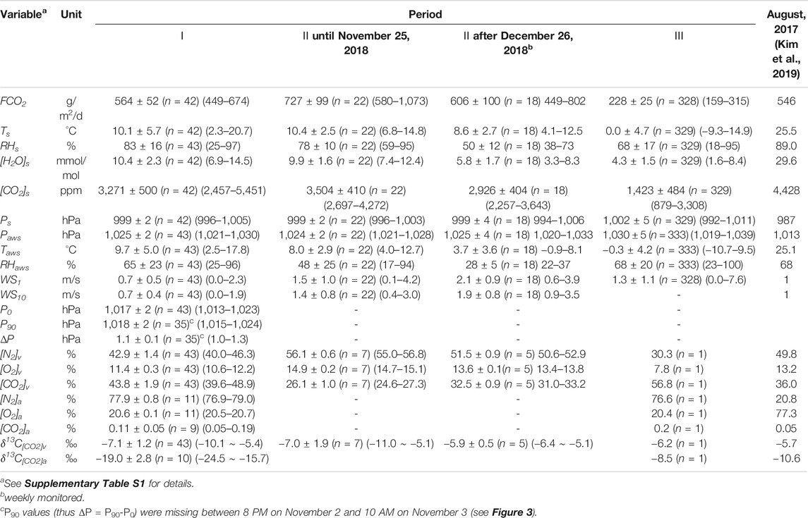
TABLE 1. Measurement results (mean ± standard deviation and range). ‘n’ represents the number of measurements.
Methodology
This study was conducted around the M17 point in Figure 1A found by a preliminary study on the spatial variation of FCO2 around the CO2-rich wells and springs with 50 –100 m spacing within 1 km2 (Kim et al., 2019). Among a total of 94 points, M17 was the only point to show geogenic CO2 outflow through the soil layer. FCO2 was detected up to 546 g/m2/d, while the soil CO2 concentration at a depth of 60 cm ([CO2]v) and its carbon isotope (δ13C[CO2]v) were 36.0% and -5.7‰, respectively at M17 in summer, 2017 (Table 1), which were much higher than the values of biogenic origin (average FCO2 of 44.9 g/m2/d, [CO2]v of 0.7% and δ13C[CO2]v of −25.2‰) observed at 79 samples in the study area (Kim et al., 2019).
Three Periods
Field works were conducted through three periods Ⅰ (from November 2 to 5, 2018), Ⅱ (November 19, 2018 to January 30, 2019), and Ⅲ (December 2 to 8, 2019) (Table 1; Supplementary Figure S2). Monitoring during the periods Ⅰ and Ⅲ was conducted to assess the background level of FCO2 and CO2 concentration in soil gas ([CO2]v), while FCO2 and [CO2]v were investigated during the period Ⅱ to assess the effect of a 2.1 M earthquake nearby (i.e., 7.8 km southwest and 20 km deep) on FCO2.
Note that there is no long-term automated FCO2 measurement system in the study area unlike other seismic or volcanic areas (e.g., Chiodini et al., 2001; Camarda et al., 2016; Morita et al., 2019) because FCO2 is not a big concern. Besides, the study area is a private land. Thus, data were missing between periods, and measurement frequency varied at each period (Supplementary Figure S2) depending on the situations in the field (e.g., accessibility, power supply). Specifically, FCO2 measurement and soil gas sampling were conducted simultaneously every 2 h during the period Ⅰ. Atmospheric air samples were collected in an 8-h interval approximately 1 m above the surface. Two weeks after the period Ⅰ ended, a 2.1 M earthquake occurred. Thus, further investigations for FCO2 and soil gas were conducted since about 12 h after the earthquake occurred (period Ⅱ). FCO2 was measured three times a day (at 14:00, 15:00, and 16:00), while soil gas samples were taken once a day (around at 14:00) until November 25. Then FCO2 and soil gas were monitored once a week between December 26, 2018 and January 30, 2019 (Table 1). Lastly, FCO2 was frequently (every 30 min) measured for a week from 00:30 December 2 to 22:30 December 8, 2019 (period Ⅲ). Soil gas and atmospheric gas samples were collected once at 15:00 on 8 December, 2019 for comparison.
The FCO2 measurement point during the period Ⅲ was not exactly the same as M17, and about 30 cm away from M17 (called M17–1 hereafter) because the flux measurement device (i.e., LI-COR) had to be reinstalled in December, 2019 and we did not expect that the small spatial distance (i.e., 30 cm separation) affected the FCO2 measurement. In contrast, [CO2]v was investigated from the same tube (M17v) installed in August 2017 by Kim et al. (2019) for all three periods.
Sampling and Measurement
FCO2, compositions of soil gas and atmospheric air, and their stable carbon isotopes (δ13CCO2) were monitored. In addition, gas pressures were measured at a depth of 90 cm (P90) and on the surface (P0) during the period Ⅰ. Meteorological parameters were obtained from an automatic weather station (AWS) of the Korea Meteorological Administration (KMA) near the study area (about 10 km away). All the measurements and their devices were summarized in Supplementary Table S1. FCO2, P0, and P90 measurements (CO2flux and Gas Pressure Measurement) and gas sampling and analysis (Ga Sampling and Analysis) were detailed below.
CO2 flux and Gas Pressure Measurement
A PVC collar (height of 11.5 cm and inside diameter of about 20 cm) was implanted into the soil, on which a bottom-opened chamber was placed (Figure 1C). Then pressure (Ps; hPa), temperature (Ts; °C), relative humidity (RHs; %), CO2 concentration ([CO2]s; ppm), and water vapor mole fraction ([H2O]s; mmol/mol) in the soil chamber were measured for 2 min by a built-in infrared gas analyzer using LI-COR 8100A (LI-COR Inc. Lincoln, NE, USA). FCO2 (g/m2/d) was calculated by Equation 1 as Jung et al. (2014):
where k is a unit conversion factor (3.80 g·s/μmol/d), R is the universal gas constant (8.31 m3·Pa/K/mol), S is the soil surface area (herein, 317.8 cm2 for the about 20 cm diameter chamber), V is the system volume (i.e., the sum of the chamber volume and the extra volume by a offset), P, T, and [H2O] are the initial Ps, Ts, and [H2O]s, respectively, and d[CO2]/dt is the rate of change in [CO2]s for the 2-min measurement.
Pore gas pressure (P90) and atmospheric pressure (P0) were monitored using a pressure transducer (BAT® geosystem). A porous filter tip was connected to the end of a 2.54 cm diameter pipe and then installed to a target depth (i.e., 90 cm). Then the pressure transducer with a needle was poked to the rubber on the top of the filter tip. Pressures were measured at a 1-min interval over the whole survey period Ⅰ. However, 30-min average values of P90 and P0 were used when the relationships with other measurements were assessed. In other words, P90 and P0 data (thus ΔP = P90 - P0) were taken for 15 min before and after the FCO2 measurement, respectively and then averaged for the 30 min.
Ga Sampling and Analysis
Soil gas samples were taken using a Teflon tube which had the outer diameter of 0.64 cm and was embedded down to 60 cm below the surface with the AMS Gas Vapor Probe (AMS, Inc., USA). Atmospheric air samples were collected 1 m above the surface. Soil gas and atmospheric air samples were purged for 5 min using a portable Masterflex E/S peristaltic pump (Cole-Parmer Instruments, USA) and then collected in a 1 L multi-layered Tedlar bag (Restek©, USA). Soil gas duplicates were collected once a day (at 14:00; n = 4) during the period Ⅰ to double check the results of δ13C[CO2]v analysis, with connecting the y-shaped adapter at the end of the sampling tube.
The carbon isotope of CO2 (δ13CCO2) in the gas samples were analyzed by the Picarro G2121-i isotope and gas analyzer (Picarro Inc., USA) at the Korea Institute of Geoscience and Mineral Resources (KIGAM). The Picarro cavity ring-down spectroscopy (CRDS) was calibrated by IAEA standard materials (δ13CCO2 = 2.492, −5.764, −47.321‰) before analyzing samples. All gas samples were purged for 10 min with laboratory air and then analyzed for 15 min to avoid the memory effect. Results were expressed relative to the international V-PDB standard. The soil gas duplicates (n = 4) obtained during the period Ⅰ and a soil gas sample obtained during the period Ⅲ were analyzed by Thermo Fisher Delta VTM IRMS (isotope ratio mass spectrometer) at Beta Analytic Inc. (Miami, USA) for comparison.
Gas compositions (N2, O2, and CO2) were determined by the Agilent 490 Micro Gas Chromatograph (GC) at KIGAM. Before the laboratory analysis, two columns in GC (i.e., CP-Molsieve 5A column for N2 and O2 and PoraPLOT U column for CO2) were calibrated by three different standards (CO2 = 49.98; 5.00; 0.04%: Rigas©, Korea). Each sample was analyzed at least three times, and the coefficient of variation was less than 0.9% for CO2.
Statistical Analysis and CO2 Solubility Calculation
Simple statistical analyses were applied for each period because of discontinuous and short-term observations at different intervals. First, Pearson correlation coefficients (
Second, autocorrelation of time series was assessed to find the periodicity for the data obtained during the periods Ⅰ and Ⅲ (Supplementary Figures S3, S4). Cross-correlation coefficients (
where
In addition, the amount of CO2 degassing from a CO2-rich aquifer was estimated by calculating the variation in CO2 solubility in groundwater due to the variation in pressure, salinity and temperature based on the method by Duan and Sun (2003).
Results
Background Levels
Measurements during the periods Ⅰ and Ⅲ were compared to assess the background levels of FCO2 and soil gas compositions (Table 1) and their relations with environmental variables (Tables 2, 3). Table 4 showed
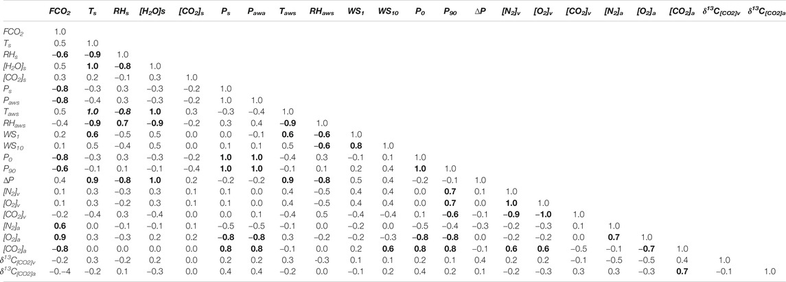
TABLE 2. Pearson correlation coefficients during the period Ⅰ. Absolute values ≥0.6 are in bold.
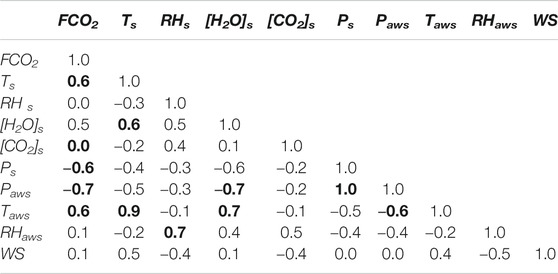
TABLE 3. Pearson correlation coefficients during the period Ⅲ. Absolute values ≥0.6 are in bold.
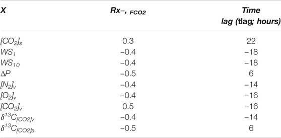
TABLE 4. Cross-correlation coefficients with a non-zero time lag during the period Ⅰ. See Supplementary Figure S5 for cross-correlation functions.
CO2 Flux
The average FCO2 during the period Ⅰ was 564 g/m2/d and ranged from 449 to 674 g/m2/d, which was similar to 546 g/m2/d obtained at M17 in August 2017 (Table 1) and quite high compared to FCO2 in the other 93 points (7.5–118 g/m2/d) in the study area measured by Kim et al. (2019) and in typical normal soil systems (∼40 g/m2/d) suggested in Ascione et al. (2018). Meanwhile, FCO2 during the period Ⅲ ranged between 159 and 315 g/m2/d (average of 228 g/m2/d), which was higher than those in the 93 points of Kim et al. (2019) and in typical normal soil systems by Ascione et al. (2018), but much lower than those during the period Ⅰ in 2018 and that in August, 2017 (Table 1). [H2O]s and [CO2]s were also lower than those during the period Ⅰ (Table 1; Figure 2). Besides, during the period Ⅰ, Ts, 1/RHs, [H2O]s, and ΔP increased daytime and decreased at night (Figures 2, 3 and Supplementary Figure S3), while the diurnal variation of [H2O]s was not clear during the period Ⅲ (Figure 2D and Supplementary Figure S4), especially until December 6, 2019 when the temperature was lowered down to −10°C and the pressure exceeded 1,010 hPa (Figures 2B,F). RHs (
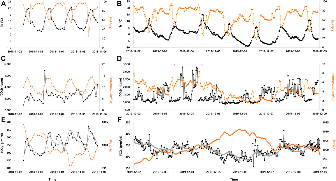
FIGURE 2. Temporal comparison of temperature (Ts; °C), relative humidity (RHs; %) in (A,B), CO2 concentrations ([CO2]s; ppm), water vapor mole fraction ([H2O]s; mmol/mol) in (C,D), and pressure (Ps; hPa) in the chamber and calculated CO2 flux (FCO2; g/m2/d) in (E,F) during the periods Ⅰ (left) and Ⅲ (right). In (E,F), the gray line addresses the FCO2 estimated using Taws and Paws in Equations 3, 4, respectively. Note that [CO2]s, [H2O]s, FCO2, and Ps have different scales between two periods. The red arrow in (D) indicates the time of rapid increases in [CO2]s.
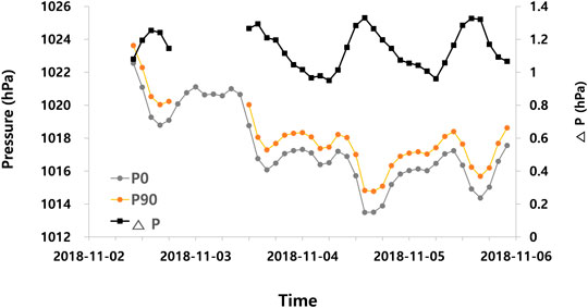
FIGURE 3. Pressures at surface (P0; hPa) and at a depth of 90 cm (P90; hPa) measured by the BAT® geosystem and the pressure difference between P0 and P90 (ΔP = P90-P0; hPa) during the period Ⅰ.
Despite the different ranges in FCO2 at each period, FCO2 had significant correlations with Ts, [H2O]s, Taws, Ps and Paws at both periods (Tables 2, 3). FCO2 increased with increasing [H2O]s, Ts and Taws but decreased with Ps and Paws. In addition, P0 and P90 were negatively correlated with FCO2 during the period Ⅰ. The negative relation of FCO2 with Paws was explained by the fact that a decrease in barometric pressure increases the pressure gradient of the ground, which subsequently enhances the viscous gas flux (Rogie et al., 2001; Granieri et al., 2003; Morita et al., 2019). The positive relation with Taws on the short time scale was explained as the effect of variations in soil gas diffusivity with air temperature as well as surficial biological productivity (Camarda et al., 2016 and references therein). The positive effect of [H2O]s can be explained by its positive relationship with Ts and Taws and negative with Ps and Paws in Tables 2, 3, and will be further discussed in Environmental Parameters regarding the usefulness of the environmental parameters obtained in the chamber.
Soil Gas and Air
CO2 concentrations in the soil gas obtained at a depth of 60 cm ([CO2]v) ranged from 39.6 to 48.9% (average = 43.8%) during the period Ⅰ (Figure 4A), which were slightly higher than that measured in August, 2017 (36.0%) but lower than that during the period Ⅲ (56.8%) in Table 1. δ13C[CO2]v for the soil gas was between −10.1 and −5.4‰ (average = −7.1‰) during the period Ⅰ and was −6.2‰ during the period Ⅲ, which were a little lower than the value (−5.7‰) obtained in August, 2017 (Figure 4A; Table 1). However, the variations in δ13C[CO2]v were insignificant and the δ13C[CO2]v values were relatively high compared to the δ13C[CO2]v of biogenic origin in the study area between −32.0 and −13.0‰ (average −25.2‰) in Kim et al. (2019).
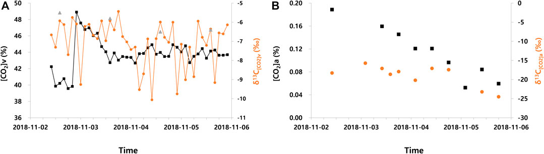
FIGURE 4. Temporal changes of (A) CO2 concentrations measured at a depth 60 cm ([CO2]v) and its δ13C[CO2]v; (B) CO2 concentrations in air samples ([CO2]a) and its δ13C[CO2]a during the period Ⅰ. Gray triangles in (A) show the δ13C[CO2]v values determined by the Beta Analytic Inc. (n = 4) for cross-checking.
[CO2]v did not show a distinct diurnal variation during the period Ⅰ (Figure 4A) similar to FCO2 and [CO2]s that showed the pattern out of the diurnal variation during both periods I and Ⅲ unlike Ts, RHs or [H2O]s (Figure 2; Supplementary Figures S3, S4). [CO2]v was not linearly correlated with either FCO2 (
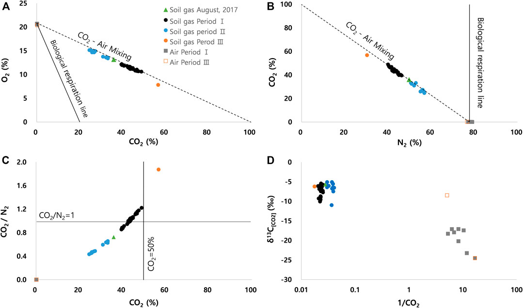
FIGURE 5. Compositions and stable carbon isotopes (δ13C[CO2]) of soil gas and atmospheric air. The relationships between CO2 and O2(A) and between N2 and CO2(B) (after Romanak et al., 2012). Dotted lines represent the mixing between atmospheric air concentrations measured in this study and 100% geogenic CO2, while solid lines represent the biological respiration in (A,B). (C) CO2/N2 vs. CO2; (D) 1/CO2 vs. δ13C[CO2] (after Sun et al., 2018). The soil gas data in August 2017 is from Kim et al. (2019).
It is noticeable that both [CO2]v and [CO2]s showed a rapid increase during the period Ⅰ with the time lag of about 12 h. Specifically, [CO2]v rapidly increased from 39.8 to 48.9% at 22:00 on November 2 (Figure 4A), while [CO2]s increased from 0.3 to 0.5% at 10:00 on November 3 (Figure 2C). Consistently, the cross-correlation analysis showed that the correlation between [CO2]v and [CO2]s increased up to 0.55 at the time lag of -12 h in Supplementary Figure S5 from zero in Table 2, and suggested the transport rate of approximately 60 cm/12 h. [CO2]s occasionally showed rapid increases during the period Ⅲ as well, in particular around December 4 (see the red arrow in Figure 2D), whereas [CO2]v measurements were not available for comparison.
Meanwhile the CO2 concentrations in the air samples ([CO2]a) measured during the periods Ⅰ (0.05–0.19%) and period Ⅲ (0.20%) in Figure 4B and Table 1 showed high values compared to a reported atmospheric CO2 composition (0.04%) and the value previously detected in the study site (0.05%). [CO2]a was negatively correlated with FCO2 (
After the Earthquake
FCO2 increased up to 1,073 g/m2/d by a factor of two approximately 12 h after the earthquake (Figure 6 and Supplementary Figure S2), which was much higher than the sum of mean (μ) and 2 times standard deviation (2σ) of FCO2 during the period Ⅰ (μ + 2σ; 668 g/m2/d). Besides, relatively high FCO2 was observed on November 25, 2018 (836 g/m2/d) and January 23, 2019 (802 g/m2/d) (Figure 6). Those high FCO2 values were not observed either during the period Ⅰ or in the previous study at M17 (Table 1).
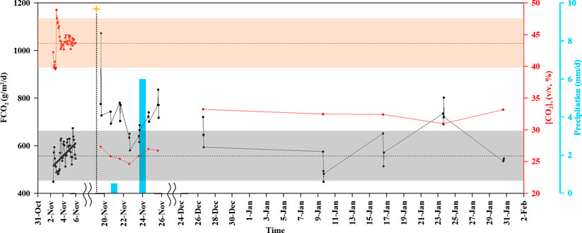
FIGURE 6. Temporal changes of CO2 flux (FCO2) and CO2 concentrations measured at a depth 60 cm ([CO2]v) before and after the 2.1 M earthquake (yellow star) occurred on November 19, 2018. The shaded areas cover the mean (μ; dotted line) ± two times standard deviation (2σ) of the period Ⅰ (Table 1). The solid thick line represents the linear regression (r2 = 0.3).
The high FCO2 seemed to be related with [CO2]s (Figure 7;
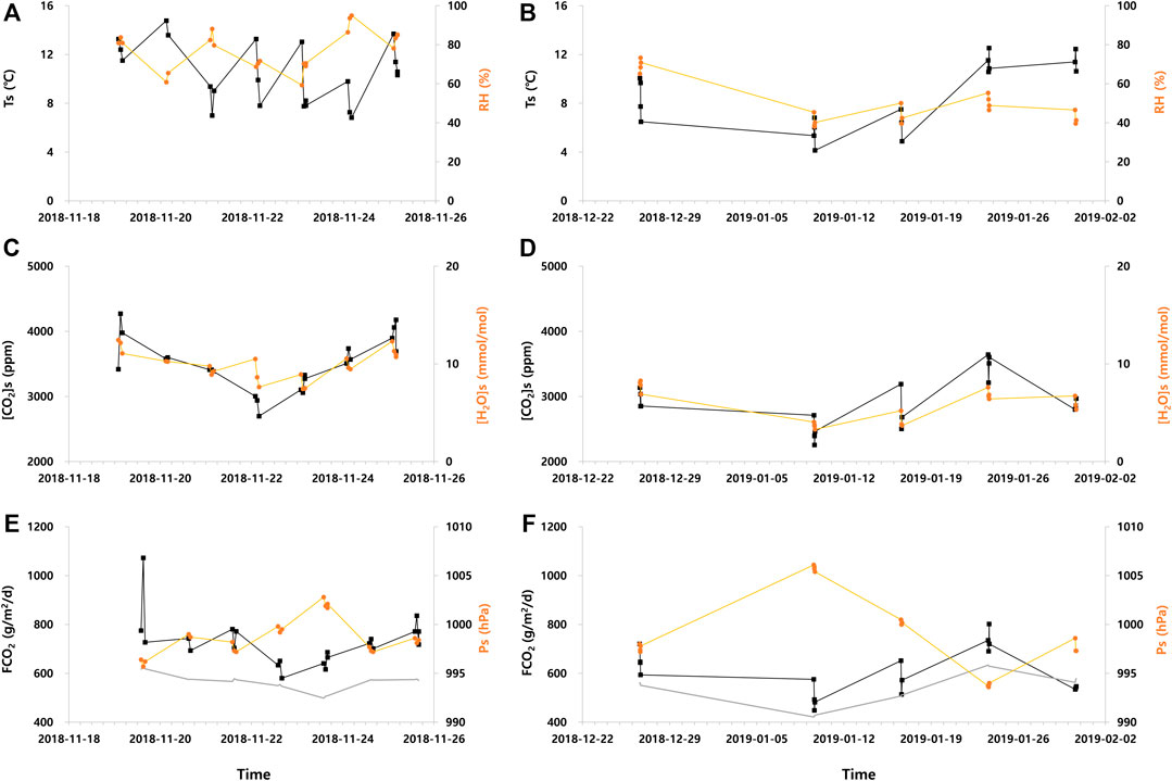
FIGURE 7. Temporal comparison of temperature (Ts), relative humidity (RHs) in (A,B), CO2 concentrations ([CO2]s), water vapor mole fraction ([H2O]s) In (C,D), and pressure (Ps) in the chamber and calculated CO2 flux (FCO2) In (E,F) during the period Ⅱ. In (E,F) the gray line addresses the FCO2 estimated using Taws and Paws in Equation 3. Note that the left (until November 25, 2018) and right figures (after December 26, 2018) have different scales of the x axis (time).
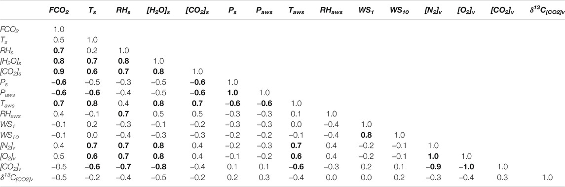
TABLE 5. Pearson correlation coefficients during the period Ⅱ. Absolute values ≥0.6 are in bold.
Besides, it was observed that the relative humidity (RH) in the chamber (RHs) and from the AWS (RHaws) were positively related with FCO2 during the period Ⅱ (
Discussion
Source of CO2
Scatter plots of soil gas compositions revealed that the soil gas was the mixture of atmospheric air and geogenic CO2 (Figure 5). Specifically, the CO2 vs. O2 was plotted on the air-CO2 mixing line (Figure 5A), while the N2 vs. CO2 was not on the biological respiration or CH4 oxidation (Figure 5B). Besides, the consistent δ13C[CO2]v regardless of the season and the δ13C[CO2]v ranges (Figure 5D) indicated a deep-seated CO2 source despite the different proportion of CO2 in soil gas at each period as the δ13CCO2 of geogenic CO2 is reported to be −6‰ in Baines and Worden (2004) and −9.7 ∼ −2.7‰ (−6.5 ± 2.5‰) in Sano and Marty (1995). In contrast, the δ13CCO2 from the microbial decomposition of C3 plants generally ranges between −34 and −23‰ (Faure, 1998) and seasonally changes due to the change in biological activities (White and Corfield, 2006; Zhu et al., 2019). FCO2 did not show the diurnal variation (Supplementary Figures S2–S4), and had a significantly negative relation with barometric pressure (Tables 2, 3, 5), which also indicates the geogenic CO2 emission in the study site (Camarda et al., 2019). At the measurement site around M17, the geological FCO2 seems to exceed the microbial respiratory FCO2 by several orders of magnitude as in the sites with high CO2 concentrations in Vodnik et al. (2009).
During the period Ⅰ, P90 was always higher than P0 (Figure 3). The positive ΔP indicates that the atmospheric air did not intrude and dilute [CO2]v at the measurement point (M17v). Instead, the mixing with air seemed to be diffusive at M17v due to concentration gradients with depth, which may be affected by the barometric pressure given that P90 was synchronized with P0 (Figure 3). Besides, the geogenic CO2 uprising could be mixed with soil gas influenced by the atmospheric air in the vadose zone. According to Massmann and Farrier (1992) and Chen et al. (2020), the changes in barometric pressure migrate air into the vadose zone. Air intrusion due to the barometric pressure fluctuation depends on soil characteristics, the thickness of vadose zone, and climate (Massmann and Farrier, 1992; Auer et al., 1996).
Meanwhile, δ13C[CO2]a was widely ranged particularly during the period Ⅰ (Figure 4B) probably due to various sources of CO2 in the air 1 m above the surface. A CO2 source in the air seemed to be geogenic given high [CO2]a values up to 0.2% (Table 1), the positive relation between [CO2]a and δ13C[CO2]a (
Factors to Control Geogenic CO2 Flux
The variation in geogenic FCO2 depends on soil properties (e.g., air permeability and diffusion coefficient), prevailing mechanisms of CO2 transport (e.g., advection and diffusion), environmental parameters (e.g., air pressure and temperature), and deep-seated CO2 supply via endogenous processes (e.g., volcano and tectonic activity). We discussed the factors controlling the temporal variations of FCO2 in relation to time-variant geogenic CO2 supply due to exploitation of CO2-rich water (Time-Variant Supply of Geogenic CO2), the effect of environmental variables including precipitation (Environmental Parameters), and the prevailing mechanisms of CO2 transport (Prevailing Mechanisms of CO2 Transport). Besides, the difference between the periods Ⅰ and Ⅲ was discussed with respect to the spatial variability of FCO2 (Heterogenous Transport of Geogenic CO2). Soil properties could not be investigated in this private land.
Time-Variant Supply of Geogenic CO2
The geogenic CO2 supply seemed to be variant with time given the irregular increases of [CO2]s (i.e., CO2 concentration in the chamber 2 min after closing the chamber in Figure 2) regardless of environmental variables (Tables 2, 3). According to Kim et al. (2019), CO2 gas in the study area forms by degassing from the water table of a CO2-rich aquifer and transports toward the M17 site and leaks at M17 via the voids surrounding the well w-2. The amount of CO2 degassing is expected to be time-variant because the CO2-rich water is taken from w-2 by countless people, which changes the groundwater level and subsequently the fluid pressure, affecting the amount of CO2 degassing (Duan and Sun, 2003). The time-variant CO2 degassing seemed to alter [CO2]v and the CO2 gradient in the subsurface, and subsequently [CO2]s, for instance with the time lag of −12 h between M17v and M17(Supplementary Figure S5E) and consequently FCO2 with the time lag of −16 h (Table 4) during the period Ⅰ.
The impact of pressure variation on degassing was quantitatively compared to that of temperature and salinity in Table 6 because the saline fluid in the deep part can rise temperature and salinity as well as pressure of groundwater. The salinity was assumed to be low (100–150 mg/L) because the CO2-rich water in the study area was characterized by low pH and electrical conductivity (EC), probably due to short (<35 years) reaction times between water and rocks despite a large amount of CO2 inflow into the aquifer (Kim et al., 2008; Chae et al., 2016). According to Chae et al. (2016), the temperature and salinity (EC) of the CO2-rich water from w-2 varied between 11.6 and 15.8°C and between 108 and 175 μS/cm for 14 months, respectively. Table 6 shows that the change in CO2 solubility (i.e., degassing) is more influential by the pressure variation than by the temperature or salinity in the study site.
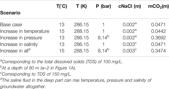
TABLE 6. Sensitivity analysis of CO2 degassing from a CO2-rich water.
When the water is pumped and thus the water pressure drops, gas bubbles occurs in CO2-rich water. Subsequently the gas release ceases and the gas dissolved in the CO2-rich water is being released as a result of a slow diffusion process (Kouznetsov et al., 2002). The “bubbly” stage may be resumed at shaking (see Possible Causes of a High CO2 Emission During the Period Ⅱ). The changes in the water table also affect FCO2in the vadose zone as in Schroder et al. (2017) who found the FCO2distribution shifted between two CO2 release tests due to the changes in groundwater depth in wet and dry season. The low water table in dry season facilitates lateral CO2 migration, reducingFCO2 along a wellbore. The quantitative assessment of the effect of pressure variation caused by water usage on the CO2 degassing (and subsequently on FCO2) in the study area remains future work due to little information on the water table and the amount of water consumption at w-2.
In addition, Chae et al. (2016) speculated dry CO2 flowing directly into the aquifer of w-2 (80 m depth) from the magmatic origin, since the study site is located at the geologic boundary between gneiss and granite (Figure 1A) and unknown fractures may exist around the study area given the small earthquakes (Figure 1B) and CO2-rich waters (Supplementary Figure S1), although none has been reported within 13 km around the study area. According to Kerrick and Caldeira (1998), the plutonic-metamorphic belt can be a source area to emit CO2 to the atmosphere. In fact, Yu et al. (2015) observed the temporal variation of CO2 supply to the aquifer for 48 h in a CO2-rich spring (s-2 in Figure 1A), which decreased pH and increased total dissolved inorganic carbon (TDIC) and δ13CTDIC and might further cause the temporal variation of [CO2]v, [CO2]s, or FCO2.
Environmental Parameters
We found the significant influence of air temperature (Taws, Ts) and pressure (Paws, Ps) to FCO2 at all periods as the previous studies (Chiodini et al., 1998; Granieri et al., 2003; Carapezza et al., 2011; Camarda et al., 2016; Morita et al., 2019). The temperature was correlated with FCO2 probably due to the effect of temperature to soil gas diffusivity near the M17 site, and not due to the biological effect in November (late fall during the period Ⅰ) and December (winter during the period Ⅲ) in South Korea (Camarda et al., 2016 and references therein). In particular, the high [CO2]v at M17v during the period Ⅲ suggested the accumulation of geogenic CO2 in the subsurface due to low soil gas diffusion at cold weather.
Ts and Ps were highly related with Taws and Paws respectively (
which had r2 = 0.65 and p = 0.00 in Equation 3 and r2 = 0.53 and p = 0.00 in Equation 4, supporting the significant effects of Taws and Paws to FCO2. However, microclimates may greatly affect some environmental parameters. For instance, the wind speed (WS) from the AWS did not influence FCO2 (Tables 2, 3, 5), probably because WS, which is sensitive to topography (Helbig et al., 2016), was not measured near the measurement point. Table 4 shows the negative correlation of FCO2 with WS at the time lag of −18 h. According to Carapezza et al. (2011), the negative effect of WS reflects that the gas is confined underground under strong wind conditions.
In addition to Ts and Ps, [H2O]s (i.e., water vapor mole fraction in the chamber 2 min after closing the chamber), showed significant correlations with FCO2 (
On the other hand, the relative humidity (RH) was positively related with FCO2 during the period Ⅱ (e.g.,
Prevailing Mechanisms of CO2 Transport
The high FCO2 and its high correlation with Paws indicate that the study site has a non-negligible advective component (Hernández et al., 2001; Ascione et al., 2018). Similarly, Kim et al. (2019) showed that the M17 site was located in the high-advection zone using the relationship between FCO2 and [CO2]s suggested by Jung et al. (2014). The negative correlation between P90 and [CO2]v (Table 2) and the positive ΔP (1.0–1.3 hPa in Table 1; Figure 3) and thus the pressure gradient in the range of 1.1 and 1.4 hPa/m during the period Ⅰ also suggest the advective flow upward in the unsaturated soil. Takle et al. (2004) showed that pressure differences between −15 and 15 Pa at depths of 0–60 cm caused FCO2 exceeding diffusional fluxes due to pressure pumping. According to Altevogt and Celia (2004), the leakage rate of 0.1 g/m s to 100 g/m s were reached at a CO2 source with the vertical pressure gradient of 0.18–49.65 hPa/m adjacent to the source boundary.
However, FCO2 was affected by air temperature and [H2O]s as well as air pressure in Tables 2, 3, 5, implying that the diffusive transport of CO2 is also significant in the study site (Camarda et al., 2019). Accordingly, temperature gradient might affect the pressure gradient of 1.1 and 1.4 hPa/m during the period Ⅰ, while the gradient was not measured. In addition, [CO2]v showed different temporal changes from FCO2 during the period Ⅰ in Figures 2E, 4A and its correlation with FCO2 increased at the time lag of −16 h in Table 4. Moreover, soil CO2 seems to mainly form through degassing of a CO2-rich aquifer and the degassing may vary depending on the pressure variation in the aquifer for w-2 (Table 6).
Thus, it can be concluded that the advection is dominant at the near surface, while the transport of geogenic soil CO2 is diffusive-dominated in the vadose zone by the CO2 gradient. Similarly, Kim et al. (2018) observed that CO2 concentrations measured at 15 cm depth were significantly lower than those measured at 60 cm depth, as the CO2 gas escaped quickly into the atmosphere at the ground surface due to the atmospheric pressure effect at an inject test, for which approximately 1.8 t CO2 was injected at 2.5 m depth with a CO2 release rate of 6 L/min. Rillard et al. (2015) showed that the advective flux between an injection point and the surface through a preferential path was the dominant gas transport process during the injection phase because it was difficult to avoid a slight overpressure at the injection point. Altevogt and Celia (2004) determined the diffusive flux as well as the slip and Darcy fluxes associated with natural CO2 leakage into the vadose zone based on a two-dimensional numerical model, and showed that the mole fraction-driven flux played an important role in the development of the CO2 plume even in situations where pressure-driven advection was the dominant flux mechanism.
Heterogenous Transport of Geogenic CO2
FCO2 was in different ranges (Table 1) and had different correlations with measurements during the periods Ⅰ and Ⅲ (Tables 2, 3) probably because the measurement points were not exactly the same but at the 30 cm separation between M17 (period Ⅰ) and M17–1 (period Ⅲ), implying the spatial variability of FCO2, as reported by other researchers including Annunziatellis et al. (2008) and Ascione et al. (2018). Similar to this study result, Annunziatellis et al. (2008) mentioned a test showing a change of more than one order of magnitude over only 30 cm. However, the spatial difference in FCO2 at the centimeter scale was not expected before the study area, and the extreme spatial variability of FCO2 needs to be further studied in the study area.
Note that the different FCO2 between November (period Ⅰ) and December (period Ⅲ) cannot be explained by the seasonal variation, given the similar FCO2 between August (summer) in 2017 and November (fall) in 2018 despite distinct climate conditions. We acknowledge that the low FCO2 might reflect the weather condition given the low temperature (Ts) and high pressure (Ps) during the period Ⅲ (Figure 2) and their positive and negative influence on FCO2 respectively (Tables 2, 3). However, the different ranges in FCO2 as well as in [H2O]s and [CO2]s between the periods Ⅰ and Ⅲ in Figure 2 imply that the effect of heterogeneous CO2 transport in the vadose zone is stronger than the weather effect. In addition, the FCO2 estimated using Equation 3 was much higher than the measured FCO2 during the period Ⅲ (Supplementary Figure S6).
Possible Causes of a High CO2 Emission During the Period Ⅱ
The FCO2 value of 1,073 g/m2/d was exceptionally high, exceeding the μ + 2σ of the period Ⅰ (Figure 6). Besides, FCO2 measurements were much higher than the estimations using Equation 3, in particular until November 25, 2018 (Figures 7E,F), implying the effect of factors other than Taws and Paws. Meanwhile, [CO2]v rapidly decreased after the earthquake. This anomalously high FCO2 peak and sudden decreases in [CO2]v during the period Ⅱ cannot be explained by the environmental parameters given similar climate conditions (Table 1), and imply a high CO2 emission, causing that FCO2 was negatively related with [CO2]v (r = −0.5 in Table 5). In addition, [CO2]s was highly correlated with FCO2 (
Emission Scenario
We suggest that vibrations caused by the earthquake induced the soil gas to transport to the surface, with rapidly decreasing [CO2]v and increasing [CO2]s and FCO2 since the study site is located between the geologic boundary (Figure 1) and unknown fracture may exist, while CO2 gas probably forms by degassing of a CO2-rich aquifer and leaks through the well (w-2) casing in the shallow (<80 m) subsurface given no high flux except M17 near w-2. Earthquake might increase air permeability by a change in site features or modification of the structural parts of the well (w-2) from which the CO2 originates. Besides, mechanical processes, including vibrations induced by an earthquake, have been known to increase degassing of dissolved gas and to enhance the movement of gas bubbles in fractured aquifers (Kouznetsov et al., 1998; Toutain and Baubron, 1999; Manga et al., 2012), changing the physicochemical parameters of water (e.g., EC, pH, temperature, water level). According to Kouznetsov et al. (1998), degassing is related to local instantaneous ruptures in the formation fluid due to the effect of elastic waves. Nuclei of bubbles are formed in these ruptures, and gas diffusion from fluid into these bubbles takes place (Kouznetsov et al., 1998). Crews and Cooper (2014) also showed that seismic waves initiated bubble nucleation and growth in groundwater, which increased the water level in boreholes, reducing effective stress in critically loaded geologic faults, and consequently induced secondary earthquakes. Fischer et al. (2017) observed the CO2 bubbles increasing in a CO2-rich well water 4 days after a 3.5 M earthquake occurring 9 km away. The high CO2 bubble concentrations lasted for 150 days.
We acknowledge that it is difficult to determine whether the high FCO2 and low [CO2]v were caused by the earthquake because of the short-term and discontinuous data with only a small earthquake. Besides, this observation was opposite to the jumps of both FCO2 and [CO2]v in soil gas wells during the seismic activity in the active fault zones (Chen et al., 2020). We did not observe the CO2-rich water to support the emission scenario during this study. However, the impact of the small earthquake cannot be excluded for the high FCO2 during the period Ⅱ, given that FCO2 measured immediately after the earthquake was beyond the seasonal and diurnal variation of FCO2 at M17 (Table 1) and much higher than that estimated using Taws and Paws (Figure 7). Moreover, it should be noted that we began to measure FCO2 12 h after the earthquake occurred, and we might miss higher values given a synchronous sharp increase of seismicity and FCO2 in a seismically active area (Camarda et al., 2016) and the velocity of P (7–8 km/s) and S wave (4–5 km/s).
Suggestion of an Earthquake Precursor
We noted that [CO2]v rapidly increased to be 48.9% on 22:00 November 2, 2018, and then the maximum [C O2]swas observed 12 h later (Figures 2C, 4A), approximately 16 days before the earthquake (Figure 6). Besides, FCO2 had an increasing trend during the period Ⅰ (r2 = 0.3 in Figure 6), although the average FCO2 (564 g/m2/d) was similar to 546 g/m2/d obtained at M17 in August 2017 (Table 1). These temporal variations might be a precursor of the earthquake. We acknowledge that many researches have been carried out on the precursors of earthquakes, while there is no general agreement among scientists on the earthquake precursors (Tsunogai and Wakita, 1995; Hernández et al., 2001; Pérez et al., 2008; Ingebritsen and Manga, 2014). Besides, the changes in soil CO2 have been reported as a result of earthquakes or volcanic activities, rather than an earthquake precursor (Hernández et al., 2001; Troll et al., 2012). Moreover, only one earthquake case was observed in this study (Supplementary Figure S2).
However, many studies suggested the soil gas to be one of the most reliable tools to investigate earthquake precursory signals (Walia et al., 2010; Sciarra et al., 2017). For instance, Sciarra et al. (2017) suggested that crustal dilation linked to seismic activity favors the uprising of geogas toward the surface. Walia et al. (2010) showed that the spatial distribution of soil gases was useful in identifying tectonic systems since it showed a clear anomalous trend along the Hsinhua Fault. Chiodini et al. (2004) found in the Apennine that the anomalous FCO2 suddenly disappeared in a narrow band with the seismicity concentrated, and suggested that the gas accumulates in crustal traps at depth, generating CO2 overpressurized reservoirs, which induce seismicity.
Conclusion
Temporal variations of soil CO2 flux (FCO2) and soil CO2 concentration ([CO2]v) were investigated for three periods to recognize the factors controlling the temporal variation of geogenic FCO2 in a non-volcanic and seismically inactive area. The periods Ⅰ (November 2 to 5, 2018) and Ⅲ (December 2 to 8, 2019) were to assess the baseline, while the period Ⅱ (November 19, 2018 to January 30, 2019) was to survey the effect of a small (2.1 M) earthquake occurring 7.8 km away. The correlation coefficients indicated that the air pressure was the most significant controlling factor to FCO2 regardless of the periods, and the air temperature was also noteworthy.
In contrast, some environmental parameters were significantly related with FCO2 during one or two periods only, e.g., [CO2]s and [CO2]v during the period Ⅱ. In particular, the low [CO2]v but high FCO2 during the period Ⅱ implied the high emission of soil CO2 after the small earthquake, which affected the relations between some environmental parameters (e.g., [CO2]s, RHs and RHaw) and FCO2. Meanwhile, the low FCO2 during the period Ⅲ suggested the heterogenous subsurface conditions for CO2 transport at the centimeter scale, while the high [CO2]v implied the accumulation of soil CO2 in the subsurface due to low soil gas diffusion at cold weather. Based on the high FCO2, its high correlation with air temperature as well as air pressure, and the different temporal changes of [CO2]v from FCO2 including the high [CO2]v at cold weather, the study area seemed to have the diffusive transport of soil CO2 dominant in the vadose zone, while the advection near the surface.
The merit of this study is to present the temporal variation of high FCO2 of deep CO2 origin in a non-volcanic and seismically inactive area and to discuss the controlling factors, given few studies on the temporal changes of geogenic CO2 emissions in a geologically stable region, although CO2-rich water discharges. In particular, we found a rapid increase of FCO2 after the small earthquake, which implies that the global natural CO2 emission can be larger than the previous estimation. In addition, artificial vibrations (e.g., building construction and transportation vibration) may enhance natural CO2 emissions, and thus CO2-rich waters or FCO2 should be monitored to assess the effect of artificial and natural vibrations to CO2 emissions. Besides, we provided the usefulness of data in the chamber and AWS data to understand the temporal variation in FCO2.
We acknowledge however that we only observed a period (Ⅱ) with respect to an earthquake because the study area has low and sporadic seismicity and no automated FCO2 monitoring system. It was difficult to determine a cause for the high FCO2 peak and decreases in [CO2]v mostly because of short-term and discontinuous monitoring at different acquisition intervals. Thus our speculation about the effect of the small earthquake to abnormal increases in FCO2 and the applicability of [CO2]v as an earthquake precursor needs to be confirmed through a physics-based numerical modeling work and long-term monitoring data. A process-based understanding for the effects of earthquakes to FCO2 and [CO2]v remains future work. Besides, we could not clearly explain the irregular temporal variations of [CO2]s and its high correlation with FCO2 during the period Ⅱ. Thus, the carbon isotopic compositions of [CO2]s is also needed to be investigated in the next study. With defining end-member properties, the proportion of geogenic CO2 in [CO2]s should be assessed to verify the temporal variation of geogenic CO2 supply with [CO2]s. Lastly, the low FCO2 during the period Ⅲ implied the high spatial variability of FCO2. A spatially intensive FCO2 investigation close to M17 will be conducted in the near future to address the reason for heterogeneity in the centimeter scale.
Based on the temporal changes in FCO2 in this non-volcanic and seismically inactive study area, we suggest to install an automated FCO2 monitoring system in natural emission sites to understand temporal increases in natural CO2 emissions and their causes (e.g., earthquake) in geologically stable regions and consequently the global natural CO2 emission based on long-term monitoring data. In particular, the FCO2 monitoring should be complemented with the monitoring of degassing from groundwater to assess the impact of tectonic stresses because endogenous factors affect the physicochemical parameters of water as well, which subsequently changes CO2 concentrations and FCO2.
Data Availability Statement
The datasets presented in this study can be found in online repositories. The names of the repository/repositories and accession number(s) can be found below: https://zenodo.org/record/3818108#.X0c3DOR7k6Y.
Author Contributions
CK conducted the field work, wrote a first draft, and made figures. SY interpreted the data, wrote the manuscript, and made figures. Y-YO interpreted the temporal data and suggested the cross-correlation analysis. GC designed and initiated the field work, and acquired and interpreted the data. S-TY contributed to the conception and design of the work. YS supervised the field work and sample analysis. All authors contributed to discussions and revisions of the manuscript.
Funding
This research was supported by the fundamental research project of KIGAM (Korea Institute of Geoscience and Mineral resources) and was partially supported by the National Research Foundation of Korea (NRF) grant funded by the Korean government (MEST) (No. 2019R1A2C1084297) and the Korea Ministry of Environment (MOE) as K-COSEM (Korea CO2 Storage Environmental Management) Research Program.
Conflict of Interest
The authors declare that the research was conducted in the absence of any commercial or financial relationships that could be construed as a potential conflict of interest.
Acknowledgments
The authors acknowledge diligent field and laboratory works by Inhye Lee, Byeongjun Park, and Gibeom Seok.
Supplementary Material
The Supplementary Material for this article can be found online at: https://www.frontiersin.org/articles/10.3389/feart.2020.599388/full#supplementary-material.
References
Altevogt, A. S., and Celia, M. A. (2004). Numerical modeling of carbon dioxide in unsaturated soils due to deep subsurface leakage. Water Resour. Res. 40, W03509. doi:10.1029/2003WR002848
Annunziatellis, A., Beaubien, S. E., Bigi, S., Ciotoli, G., Coltella, M., and Lombardi, S. (2008). Gas migration along fault systems and through the vadose zone in the Latera caldera (central Italy): implication for CO2 geological storage. Int. J. Greenhouse Gas Control 2 (3), 353–372. doi:10.1016/j.ijggc.2008.02.003
Ascione, A., Ciotoli, G., Bigi, S., Buscher, J., Mazzoli, S., Ruggiero, L., et al. (2018). Assessing mantle versus crustal sources for non-volcanic degassing along fault zones in the actively extending southern Apennines mountain belt (Italy). GSA Bulletin 130 (9-10), 1697–1722. doi:10.1130/B31869.1
Auer, L. H., Rosenberg, N. D., Birdsell, K. H., and Whitney, E. M. (1996). The effects of barometric pumping on contaminant transport. J. Contam. Hydrol. 24 (2), 145–166. doi:10.1016/S0169-7722(96)00010-1
Baines, S. J., and Worden, R. H. (2004). The long-term fate of CO2 in the subsurface: natural analogues for CO2 storage. Geol. Soc. London Spec. Publ. 233 (1), 59–85. doi:10.1144/GSL.SP.2004.233.01.06
Burton, M. R., Sawyer, G. M., and Granieri, D. (2013). Deep carbon emissions from volcanoes. Rev. Mineral. Geochem. 75 (1), 323–354. doi:10.2138/rmg.2013.75.11
Camarda, M., De Gregorio, S., Di Martino, R. M., and Favara, R. (2016). Temporal and spatial correlations between soil CO2 flux and crustal stress. J. Geophys. Res. Solid Earth. 121 (10), 7071–7085. doi:10.1002/2016JB013297
Camarda, M., De Gregorio, S., Capasso, G., Di Martino, R. M., Gurrieri, S., and Prano, V. (2019). The monitoring of natural soil CO2 emissions: issues and perspectives. Earth Sci. Rev. 198, 102928. doi:10.1016/j.earscirev.2019.102928
Carapezza, M. L., Barberi, F., Ranaldi, M., Ricci, T., Tarchini, L., Barrancos, J., et al. (2011). Diffuse CO2 soil degassing and CO2 and H2S concentrations in air and related hazards at vulcano island (aeolian arc, italy). J. Volcanol. Geoth. Res. 207 (3-4), 130–144. doi:10.1016/j.jvolgeores.2011.06.010
Cardellini, C., Chiodini, G., and Frondini, F. (2003). Application of stochastic simulation to CO2 flux from soil: mapping and quantification of gas release. J. Geophys. Res. Solid Earth 108 (B9), 2425. doi:10.1029/2002JB002165
Chae, G., Yu, S., Jo, M., Choi, B. Y., Kim, T., Koh, D. C., et al. (2016). Monitoring of CO2-rich waters with low pH and low EC: an analogue study of CO2 leakage into shallow aquifers. Environ. Earth Sci. 75 (5), 390. doi:10.1007/s12665-015-5206-9
Chen, Z., Li, Y., Martinelli, G., Liu, Z., Lu, C., and Zhao, Y. (2020). Spatial and temporal variations of CO2 emissions from the active fault zones in the capital area of china. Appl. Geochem. 112, 104489. doi:10.1016/j.apgeochem.2019.104489
Chiodini, G., Cardellini, C., Amato, A., Boschi, E., Caliro, S., Frondini, F., et al. (2004). Carbon dioxide earth degassing and seismogenesis in central and southern italy. Geophys. Res. Lett. 31 (7), L07615. doi:10.1029/2004GL019480
Chiodini, G., Cioni, R., Guidi, M., Raco, B., and Marini, L. (1998). Soil CO2 flux measurements in volcanic and geothermal areas. Appl. Geochem. 13 (5), 543–552. doi:10.1016/S0883-2927(97)00076-0
Chiodini, G., Frondini, F., Kerrick, D. M., Rogie, J., Parello, F., Peruzzi, L., et al. (1999). Quantification of deep CO2 fluxes from Central Italy. Examples of carbon balance for regional aquifers and of soil diffuse degassing. Chem. Geol. 159 (1-4), 205–222. doi:10.1016/S0009-2541(99)00030-3
Chiodini, G., Frondini, F., Cardellini, C., Granieri, D., Marini, L., and Ventura, G. (2001). CO2 degassing and energy release at solfatara volcano, campi flegrei, italy. J. Geophys. Res. Solid Earth 106 (B8), 16213–16221. doi:10.1029/2001JB000246
Chiodini, G., Granieri, D., Avino, R., Caliro, S., Costa, A., and Werner, C. (2005). Carbon dioxide diffuse degassing and estimation of heat release from volcanic and hydrothermal systems. J. Geophys. Res. Solid Earth 110 (B8), B08204. doi:10.1029/2004JB003542
Ciotoli, G., Bigi, S., Tartarello, C., Sacco, P., Lombardi, S., Ascione, A., et al. (2014). Soil gas distribution in the main coseismic surface rupture zone of the 1980, Ms= 6.9, Irpinia earthquake (southern italy). J. Geophys. Res. Solid Earth 119 (3), 2440–2461. doi:10.1002/2013JB010508
Ciotoli, G., Etiope, G., Marra, F., Florindo, F., Giraudi, C., and Ruggiero, L. (2016). Tiber delta CO2‐CH4 degassing: a possible hybrid, tectonically active Sediment‐Hosted Geothermal system near rome. J. Geophys. Res. Solid Earth 121 (1), 48–69. doi:10.1002/2015JB012557
Crews, J. B., and Cooper, C. A. (2014). Experimental evidence for seismically initiated gas bubble nucleation and growth in groundwater as a mechanism for coseismic borehole water level rise and remotely triggered seismicity. J. Geophys. Res. Solid Earth 119 (9), 7079–7091. doi:doi.org/10.1002/2014JB011398
Duan, Z., and Sun, R. (2003). An improved model calculating CO2 solubility in pure water and aqueous NaCl solutions from 273 to 533 K and from 0 to 2000 bar. Chem. Geol. 193 (3-4), 257–271. doi:10.1016/S0009-2541(02)00263-2
Faure, G. (1998). Principles and applications of geochemistry. Upper Saddle River, New Jersey: Prentice-Hall, Vol. 625.
Fischer, T., Matyska, C., and Heinicke, J. (2017). Earthquake-enhanced permeability–evidence from carbon dioxide release following the ML 3.5 earthquake in West bohemia. Earth Planet Sci. Lett. 460, 60–67. doi:10.1016/j.epsl.2016.12.001
Fischer, T. P., Arellano, S., Carn, S., Aiuppa, A., Galle, B., Allard, P., et al. (2019). The emissions of CO2 and other volatiles from the world’s subaerial volcanoes. Sci. Rep. 9, 18716. doi:10.1038/s41598-019-54682-1
Garcia-Anton, E., Cuezva, S., Fernandez-Cortes, A., Benavente, D., and Sanchez-Moral, S. (2014). Main drivers of diffusive and advective processes of CO2-gas exchange between a shallow vadose zone and the atmosphere. Int. J. Greenh. Gas Con. 21, 113–129.
Granieri, D., Chiodini, G., Marzocchi, W., and Avino, R. (2003). Continuous monitoring of CO2 soil diffuse degassing at phlegraean fields (Italy): influence of environmental and volcanic parameters. Earth Planet Sci. Lett. 212, 167–179. doi:10.1016/s0012-821x(03)00232-2
Helbig, N., Mott, R., van Herwijnen, A., Winstral, A., and Jonas, T. (2016). Parameterizing surface wind speed over complex topography. JGR Atmosphere 122 (2), 651–667. doi:10.1002/2016jd025593
Hernández, P. A., Salazar, J. M., Shimoike, Y., Mori, T., Notsu, K., and Pérez, N. (2001). Diffuse emission of CO2 from miyakejima volcano, japan. Chem. Geol. 177 (1-2), 175–185. doi:10.1016/S0009-2541(00)00390-9
Ingebritsen, S. E., and Manga, M. (2014). Earthquakes: hydrogeochemical precursors. Nat. Geosci. 7 (10), 697–698. doi:10.1038/ngeo2261
Jeong, C. H., Kim, H. J., and Lee, S. Y. (2005). Hydrochemistry and genesis of CO2-rich springs from mesozoic granitoids and their adjacent rocks in south korea. Geochem. J. 39 (6), 517–530. doi:10.2343/geochemj.39.517
Jeong, C. H., Kim, J. G., and Lee, J. Y. (2001). Occurrence, geochemistry and origin of CO2-rich water from the chungcheong area, korea. Econo. Environ. Geol. 34, 227–241. doi:10.9720/kseg.2016.4.515
Johnson, J. W., and Rostron, B. J. (2012). “Geochemical monitoring,” in Best practices for validating CO2 geological storage: observations and guidance from the IEAGHG Weyburn-Midale CO2 monitoring and storage project. Editor B. Hitchon (Alberta, Canada: Geoscience Pub.) 119–154.
Jung, N. H., Han, W. S., Watson, Z. T., Graham, J. P., and Kim, K. Y. (2014). Fault-controlled CO2 leakage from natural reservoirs in the colorado plateau, east-central utah. Earth Planet Sci. Lett. 403, 358–367. doi:10.1016/j.epsl.2014.07.012
Kerrick, D. M., and Caldeira, K. (1994). Metamorphic CO2 degassing and early cenozoic paleoclimate. GSA Today 4 (3), 57–65.
Kerrick, D. M., and Caldeira, K. (1998). Metamorphic CO2 degassing from orogenic belts. Chem. Geol. 145 (3-4), 213–232. doi:10.1016/S0009-2541(97)00144-7
Kerrick, D. M., and Caldeira, K. (1993). Paleoatmospheric consequences of CO2 released during early Cenozoic regional metamorphism in the Tethyan orogen. Chem. Geol. 108 (1-4), 201–230. doi:10.1016/0009-2541(93)90325-D
Kerrick, D. M., McKibben, M. A., Seward, T. M., and Caldeira, K. (1995). Convective hydrothermal CO2 emission from high heat flow regions. Chem. Geol. 121 (1-4), 285–293. doi:10.1016/0009-2541(94)00148-2
Kihm, Y. H., and Kim, J. H. (2003). Structural characteristics of the central Ogcheon Belt, South Korea: orogen-parallel tectonic transport model. J. Asian Earth Sci. 22, 41–57. doi:10.1016/s1367-9120(03)00022-1
Kim, H.-J., Han, S. H., Kim, S., Yun, S.-T., Jun, S.-C., Oh, Y.-Y., et al. (2018). Characterizing the spatial distribution of CO2 leakage from the shallow CO2 release experiment in south korea. Int. J. Greenhouse Gas Control 72, 152–162.
Kim, J., Yu, S., Yun, S. T., Kim, K. H., Kim, J. H., Shinn, Y. J., et al. (2019). CO2 leakage detection in the near-surface above natural CO2-rich water aquifer using soil gas monitoring. Int. J. Greenhouse Gas Control 88, 261–271. doi:10.1016/j.ijggc.2019.06.015
Kim, K., Jeong, D. H., Kim, Y., Koh, Y. K., Kim, S. H., and Park, E. (2008). The geochemical evolution of very dilute CO2‐rich water in Chungcheong Province, Korea: processes and pathways. Geofluids 8 (1), 3–15. doi:10.1111/j.1468-8123.2007.00200.x
KMA (Korea Meteorological Administration) (2019). Weather information. Available at: https://www.weather.go.kr.
Kouznetsov, O. L., Simkin, E. M., Chilingar, G. V., and Katz, S. A. (1998). Improved oil recovery by application of vibro-energy to waterflooded sandstones. J. Petrol. Sci. Eng. 19 (3-4), 191–200. doi:10.1016/S0920-4105(97)00022-3
Kouznetsov, O. L., Simkin, E. M., Chilingar, G. V., Gorfunkel, M. V., and Robertson, J. O. (2002). Seismic techniques of enhanced oil recovery: experimental and field results. Energy Sources 24 (9), 877–889. doi:10.1080/00908310290086761
Lewicki, J. L., Hilley, G. E., Dobeck, L., and Spangler, L. (2010). Dynamics of CO2 fluxes and concentrations during a shallow subsurface CO2 release. Environ. Earth Sci. 60, 285–297.
Lee, H., Muirhead, J. D., Fischer, T. P., Ebinger, C. J., Kattenhorn, S. A., Sharp, Z. D., et al. (2016). Massive and prolonged deep carbon emissions associated with continental rifting. Nat. Geosci. 9, 145–149. doi:10.1038/ngeo2622
Lewicki, J. L., Hilley, G. E., Dobeck, L., and Spangler, L. (2010). Dynamics of CO2 fluxes and concentrations during a shallow subsurface CO2 release. Environ. Earth Sci. 60, 285–297.
Manga, M., Beresnev, I., Brodsky, E. E., Elkhoury, J. E., Elsworth, D., Ingebritsen, S. E., et al. (2012). Changes in permeability caused by transient stresses: field observations, experiments, and mechanisms. Rev. Geophys. 50 (2), RG2004. doi:10.1029/2011RG000382
Massmann, J., and Farrier, D. F. (1992). Effects of atmospheric pressures on gas transport in the vadose zone. Water Resour. Res. 28 (3), 777–791. doi:10.1029/91WR02766
MCT (Ministry of Construction and Transportation), KRCC (Korea Rural Community Co.), and K–Water. (2006). Groundwater basic survey in the Yeongi area. No. 11–1500000–01811–01.
Morita, M., Mori, T., Yokoo, A., Ohkura, T., and Morita, Y. (2019). Continuous monitoring of soil CO 2 flux at aso volcano, japan: the influence of environmental parameters on diffuse degassing. Earth Planets Space 71 (1), 1. doi:10.1186/s40623-018-0980-8
Mörner, N. A., and Etiope, G. (2002). Carbon degassing from the lithosphere. Global Planet. Change 33 (1-2), 185–203. doi:10.1016/S0921-8181(02)00070-X
Oliveira, S., Viveiros, F., Silva, C., and Pacheco, J. E. (2018). Automatic filtering of soil CO2 flux data; different statistical approaches applied to long time series. Front. Earth Sci. 6, 208. doi:10.3389/feart.2018.00208
Pérez, N. M., Hernández, P. A., Igarashi, G., Trujillo, I., Nakai, S., Sumino, H., et al. (2008). Searching and detecting earthquake geochemical precursors in CO2-rich groundwaters from galicia, spain. Geochem. J. 42 (1), 75–83. doi:10.2343/geochemj.42.75
R core team (2019). R: a language and environment for statistical computing. Vienna, Austria: R Foundation for Statistical Computing.
Ricci, T., Finizola, A., Barde-Cabusson, S., Delcher, E., Alparone, S., Gambino, S., et al. (2015). Hydrothermal fluid flow disruptions evidenced by subsurface changes in heat transfer modality: the la fossa cone of vulcano (Italy) case study. Geology 43 (11), 959–962. doi:10.1130/G37015.1
Rillard, J., Loisy, C., Le Roux, O., Cerepi, A., Garcia, B., Noirez, S., et al. (2015). The DEMO-CO2 project: a vadose zone CO2 and tracer leakage field experiment. Int. J. Greenhouse Gas Control 39, 302–317. doi:10.1016/j.ijggc.2015.04.012
Rogie, J. D., Kerrick, D. M., and Sorey, M. L. (2001). Dynamics of carbon dioxide emission at mammoth mountain, california. Earth Planet Sci. Lett. 188, 535–541. doi:10.1016/s0012-821x(01)00344-2
Romanak, K. D., Bennett, P. C., Yang, C., and Hovorka, S. D. (2012). Process‐based approach to CO2 leakage detection by vadose zone gas monitoring at geologic CO2 storage sites. Geophys. Res. Lett. 39 (15), L15405. doi:10.1029/2012GL052426
Sano, Y., and Marty, B. (1995). Origin of carbon in fumarolic gas from island arcs. Chem. Geol. 119 (1–4), 265–274. doi:10.1016/0009-2541(94)00097-R
Schroder, I. F., Zhang, H., Zhang, C., and Feitz, A. J. (2016). The role of soil flux and soil gas monitoring in the characterisation of a CO2 surface leak: a case study in qinghai, china. Int. J. Greenhouse Gas Control 54, 84–95. doi:10.1016/j.ijggc.2016.07.030
Schroder, I. F., Wilson, P., Feitz, A. F., and Ennis-King, J. (2017). Evaluating the performance of soil flux surveys and inversion methods for quantification of CO2 leakage. Energy Procedia 114, 3679–3694. doi:10.1016/j.egypro.2017.03.1499
Sciarra, A., Cantucci, B., and Coltorti, M. (2017). Learning from soil gas change and isotopic signatures during 2012 emilia seismic sequence. Sci. Rep. 7 (1), 1–7. doi:10.1038/s41598-017-14500-y
Sun, Y., Guo, Z., Liu, J., and Du, J. (2018). CO2 diffuse emission from maar lake: an example in changbai volcanic field, NE china. J. Volcanol. Geoth. Res. 349, 146–162. doi:10.1016/j.jvolgeores.2017.10.012
Takle, E. S., Massman, W. J., Brandle, J. R., Schmidt, R. A., Zhou, X., Litvina, I. V., et al. (2004). Influence of high-frequency ambient pressure pumping on carbon dioxide efflux from soil. Agric. For. Meteorol. 124, 193–206. doi:10.1016/j.agrformet.2004.01.014
Toutain, J. P., and Baubron, J. C. (1999). Gas geochemistry and seismotectonics: a review. Tectonophysics 304 (1-2), 1–27. doi:10.1016/S0040-1951(98)00295-9
Troll, V. R., Hilton, D. R., Jolis, E. M., Chadwick, J. P., Blythe, L. S., Deegan, F. M., et al. (2012). Crustal CO2 liberation during the 2006 eruption and earthquake events at Merapi volcano, indonesia. Geophys. Res. Lett. 39 (11), L11302. doi:10.1029/2012GL051307
Tsunogai, U., and Wakita, H. (1995). Precursory chemical changes in ground water: kobe earthquake, japan. Science 269 (5220), 61–63. doi:10.1126/science.269.5220.61
Vodnik, D., Videmšek, U., Pintar, M., Maček, I., and Pfanz, H. (2009). The characteristics of soil CO2 fluxes at a site with natural CO2 enrichment. Geoderma 150 (1-2), 32–37. doi:10.1016/j.geoderma.2009.01.005
Walia, V., Lin, S. J., Fu, C. C., Yang, T. F., Hong, W. L., Wen, K. L., et al. (2010). Soil–gas monitoring: a tool for fault delineation studies along hsinhua fault (Tainan), southern taiwan. Appl. Geochem. 25 (4), 602–607. doi:10.1016/j.apgeochem.2010.01.017
Woo, J. U., Rhie, J., Kim, S., Kang, T. S., Kim, K. H., and Kim, Y. (2019). The 2016 Gyeongju earthquake sequence revisited: aftershock interactions within a complex fault system. Geophys. J. Int. 217 (1), 58–74. doi:10.1093/gji/ggz009
Yu, S., Chae, G., Jo, M., Kim, J. C., and Yun, S. T. (2015). Assessment of CO2 discharge in a spring using time-variant stable carbon isotope data as a natural analogue study of CO2 leakage. Vienna, Austria: EGU general assembly, Vol. 17.
Zhou, X., Apple, M. E., Dobeck, L. M., Cunningham, A. B., and Spanglerc, L. H. (2013). Observed response of soil O2 concentration to leaked CO2 from an engineered CO2 leakage experiment. Int. J. Greenh. Gas Con. 16, 116–128.
Keywords: geogenic soil CO2 flux, temporal changes, controlling factors, non-volcanic and , seismically inactive, earthquake
Citation: Kim CY, Yu S, Oh Y-Y, Chae G, Yun S-T and Shinn YJ (2021) Short-Term Monitoring of Geogenic Soil CO2 Flux in a Non-Volcanic and Seismically Inactive Emission Site, South Korea. Front. Earth Sci. 8:599388. doi: 10.3389/feart.2020.599388
Received: 27 August 2020; Accepted: 26 November 2020;
Published: 15 January 2021.
Edited by:
Guodong Zheng, Chinese Academy of Sciences (CAS), ChinaReviewed by:
Jianguo Du, China Earthquake Administration, ChinaZhi Chen, China Earthquake Administration, China
Georgy Alekseevich Chelnokov, Geological Institute (RAS), Russia
Copyright © 2021 Kim, Yu, Oh, Chae, Yun and Shinn. This is an open-access article distributed under the terms of the Creative Commons Attribution License (CC BY). The use, distribution or reproduction in other forums is permitted, provided the original author(s) and the copyright owner(s) are credited and that the original publication in this journal is cited, in accordance with accepted academic practice. No use, distribution or reproduction is permitted which does not comply with these terms.
*Correspondence: Soonyoung Yu, aWFteXN5QGtvcmVhLmFjLmty
†Present address: Chan Yeong Kim, Pohang Accelerator Laboratory, Pohang, South Korea Yun-Yeong Oh, Korea National Institute of Environmental Research, Incheon, South Korea