Nonlinear Forced Change and Nonergodicity: The Case of ENSO-Indian Monsoon and Global Precipitation Teleconnections

1 Introduction

ENSO teleconnections are widely studied, but their changes resulting from external forcing, such as an increasing concentration of greenhouse gases, remain to be further explored and understood. Power and Delage (2018) provide a multi-model assessment of ENSO-precipitation teleconnection changes based on the fifth phase of the Coupled Model Intercomparison Project (CMIP5) archive. They consider, in particular, ENSO-driven precipitation anomalies in tropical regions around the globe, and assess them jointly with changes of mean precipitation. Haszpra et al. (2020a) have evaluated only the trend in the strength of ENSO-precipitation teleconnection, however, not in a multimodel ensemble but the so-called “single model initial condition large ensemble” (SMILE) CESM1-LE (Kay et al., 2015). Working with a SMILE has the advantages that the response to forcing is correctly represented in that model at least (Bódai and Tél, 2012; Drótos et al., 2015; Tél et al., 2019), and seeking a physical interpretation of changes is not faced with confusion at the outset, even if the physics depicted in that model is inaccurate or unrealistic.

The forced response is the time evolution of some ensemble-wise statistics, or, most generically, that of the probability measure carried by the climate snapshot attractor (Bódai and Tél, 2012; Drótos et al., 2015; Tél et al., 2019). The ensemble-wise statistics evaluated over the converged ensemble (Drótos et al., 2017) is in a one-to-one correspondence with the external forcing of the nonautonomous dynamical system, hence the term ‘forced response.’ For specific observables, this translates to the time evolution of any statistics evaluated with respect to an ensemble, e.g., that of mean values, standard deviations, correlation coefficients, empirical orthogonal functions (EOFs). Note that quantifiers of internal variability exhibit a forced response just as well as quantifiers of the “mean state.” The ensemble must have converged to the time-evolving snapshot attractor (Drótos et al., 2017); in the terminology of climate research, this means the correct representation of the full ensemble spread along with the absence of any drift. External forcing is defined as an explicit dependence on time of any parameter of the system (Ghil and Lucarini, 2020), which in historical and RCP runs corresponds to changes in the atmospheric composition (including greenhouse gases, anthropogenic aerosols and volcanic aerosols), land use, and solar activity (Meinshausen et al., 2011).

Without convergence, or considering a single realization, which may even correspond to observations, the state depends also on initial conditions, so that forced changes cannot be precisely disentangled from changes brought about by internal variability. In an attempt of doing this nevertheless, concerning a single realization, the standard practice is that a trend, linear or not (Franzke, 2014), is simply identified as a forced change, before possibly “anomalies,” i.e., (what is assumed to be) the internal variability is analyzed. Identifying the principal component (PC) of the leading or first empirical orthogonal function (EOF1) (Storch and Zwiers, 1999) obtained without detrending with the forced response (Kim and Ha, 2015; Pandey et al., 2020) is still somewhat arbitrary. It certainly leads to biases (Drótos et al., 2016). Yet, even with SMILEs available, it is very common to see that authors evaluate temporal statistics first–unnecessarily involving a subjective factor—and ensemble statistics afterward (Vega-Westhoff and Sriver, 2017; Carréric et al., 2020). The biases of all these approaches are certainly controlled by the magnitude of the climate change signal relative to the intensity of internal variability—a kind of signal-to-noise ratio. Computing the PC1 of EOF1 without detrending, as mentioned just above, is in fact meant to maximize the signal at least, and the EOF1 is referred to (Santer et al., 2019) as a “fingerprint” of the forced change—the spatial pattern that is supposed to be distorted by internal variability, in any single realization, the least. See (Timmermann, 1999) which is concerned rather with the minimization of the “noise.”

It is not pertinent to talk about “advantages” of temporal or ensemble methods over one another, because no situation arises when we need to decide between them. When an ensemble is available, the correct, conceptually sound ensemble method is to be applied if the forced response (including that of internal variability) is concerned. However, certainly we can make statements only about the given model.¹ Therefore, we should speak only about limitations in the respective situations of analyzing observational or modeled ensemble data.

We should note that the finite-size estimators of some statistics of basic interest are not generally unbiased—an example to appear in this work—and there might not be a universally applicable correction to the estimator to make it unbiased [unlike, e.g., the fortunate cases of the central moments (Heffernan, 1997)]. Therefore, even an ensemble-wise approach could suffer from biases in practice with the ensemble size being always finite. Some extreme value statistics are likely other examples.

Concerning teleconnections, in particular, the forced response can be identified as the time evolution of the ensemble-wise Pearson correlation coefficient (Herein et al., 2016; Yettella et al., 2018) (in a simple linear approach) between some quantities representing anomalies. The anomaly can correspond to a simple spatial (mean of a temporal) mean (Bódai et al., 2020b), but also the PC of an EOF concerning variability across the ensemble, called a snapshot EOF (SEOF) (Haszpra et al., 2020c). Haszpra et al. (2020a) take the latter approach; however, this can be extended to obtaining anomalies observing the “mutual variability,” e.g., in the sense of Maximal Covariance Analysis (MCA) (Storch and Zwiers, 1999) or Canonical Correlation Analysis (CCA) (Storch and Zwiers, 1999; Härdle and Simar, 2007). That is, with an interest in a teleconnection and its forced response, MCA and CCA—just like EOF analysis—can also be pursued concerning the variability across the ensemble, whereby we can refer to these methods as SMCA and SCCA. This is perhaps best suited to teleconnection analyses concerning two extended, possibly disconnected, regions. See an application of SMCA to studying the forced change of the coupling of JJA 200 hPa geopotential height and September sea ice concentration in (Haszpra et al., 2020b; Topál et al., 2020).

An other important example would be the relationship of the summer monsoon precipitation on the Indian subcontinent with the ENSO phenomenon which extends over the whole of the Equatorial Pacific (Wang, 2006; Mishra et al., 2012; Wang et al., 2015). In a previous publication (Bódai et al., 2020b) we examined the forced response of the ENSO-Indian monsoon teleconnection in the Max Planck Institute Grand Ensemble (MPI-GE) (Maher et al., 2019) representing the monsoon by the average JJAS precipitation over India and the ENSO by either the gridpoint- and SLP-based SOI (Southern Oscillation Index), or the areal mean of the SST in some extended area in the Equatorial Pacific. Standard choices for the latter are the Niño3, Niño4, and Niño3.4 regions. For the first time we established, via a formal hypothesis test, that standard representations of the teleconnection² strengthened in this model, both in the historical period and under the high-emission RCP8.5 forcing scenario, although not necessarily monotonically. In fact, using the SOI it was the historical period only when an increase could be detected, and, using the Niño3 index, it was rather the RCP8.5 scenario under which an increase could be detected. This raises the question whether the discrepancy is down more to 1) the physical difference between the SOI and Niño3 indices, or 2) rather that–one based on two distant gridpoints while the other on a limited region of the Equatorial Pacific–they “take somewhat different slices” of the whole ENSO phenomenon. This question is especially relevant when spatial characteristics of ENSO may also have a forced response besides the amplitude. In fact, using the Niño3.4 index, instead of Niño3, the result is closer to that using the SOI or the so-called box-SOI. With all these representations, one is able to detect the same nonmonotonicity: a temporary weakening around the turn of the millennium. In addition, both with Niño3.4 and the box-SOI changes are detected both under the historical and scenario forcing. On the one hand (I), this seems to rule out that using SST versus SLP makes much difference. We will see below that this is actually not precisely the case. On the other hand (II), it is still a question whether spatial characteristics of ENSO (in terms of SEOFs) or the whole teleconnection (in terms of SMCA or SCCA) would also change, or only the variance as reflected in the magnitudes of the PCs belonging to either of the said instantaneous (snapshot) spatial modes. These are the two basic questions that we set out here to investigate.

Furthermore, this study identifies, in terms of a regression model, three controlling factors driving the forced change of the ENSO-IM teleconnection strength. These are the ENSO variability, the coupling (i.e., the regression coefficient), and the intensity of other influences—which include but are not restricted to internal influences from the IM region and can be viewed as noise. We find that the changes of the ENSO-IM teleconnection are not driven only or dominantly by the change of ENSO variability. Nevertheless, it imprints its nonlinearity onto the teleconnection change, which might be an important source of biases (besides using a biased estimator). In particular, any nonlinearity prompts that the system should be nonergodic³ with respect to correlations, i.e., biases should exist (Drótos et al., 2016) in the temporal correlation coefficient evaluated in, say, multi-decadal time windows. Such a bias is something to bear in mind besides the ample statistical fluctuations of finite-size statistics even under a stationary climate (Bódai et al., 2020b). Nonlinearity is implied in our case by a nonmonotonic change in the ENSO variability: after a seemingly monotonic change, a decline follows in the second half of the 21st c. under RCP8.5.⁴ Given that the ensemble size is finite and not so large from the point of view of teleconnections, we develop here a statistical test whereby we can detect nonergodicity, and, subsequently, map out regions of the world where such a nonergodicity can be detected in the MPI-GE in the context of the relationship of local precipitation with ENSO.

The rest of the paper is organized as follows. In Section 2 we provide details about our methodology of analyzing the forced response of teleconnections, such as the way we pursue EOF, MCA, CCA, the definitions of a host of teleconnection representations, as well as the idea of decomposing the change of the teleconnection strength in terms of a simple regression model. In Section 3 we provide results both on spatial aspects of the forced change of the ENSO-IM teleconnections and those concerning magnitudes. Section 4 provides a comparison of the MPI-ESM with observational and reanalysis data. In Section 5 we outline our method of detecting nonergodicity and map out the world with respect to the degree of nonergodicity concerning the synoptic relationship of the local JJA precipitation with ENSO. In Section 6 we discuss and summarize our results.

2 Data and Methods

2.1 Data

The analysis is restricted to the historical and RCP8.5 simulations of the Max Planck Institute Grand Ensemble (MPI-GE, Maher et al., 2019), which is a collection of initial-condition ensemble simulations of the Max Planck Institute Earth System Model (MPI-ESM) under various forcing. The MPI-ESM is a fully coupled Earth system model, and its version 1.1.00p2, between phases 5 and 6 of the CMIP, was used to generate the MPI-GE from initial conditions that sample a long pre-industrial control run. See Maher et al. (2019) for further details. We make use of the same 63 of the 100 ensemble members as done in (Bódai et al., 2020b), due to concerns that the discarded members have not converged to the climate attractor of the model (Drótos et al., 2017).

To characterize the ENSO we make use of the 2D fields of either the Sea Level Pressure (SLP) or the Sea Surface Temperature (SST). The Indian Summer Monsoon Rain (ISMR) was calculated from the total (convective and large-scale) precipitation rate. The variable codes for SLP, SST and total precipitation rate are 134, 12 and 4, respectively. Monthly mean SLP is accessible publicly at https://esgf-data.dkrz.de/projects/mpi-ge/under variable name “psl.” The SST can be derived from the top layer of the 3D potential temperature field, whose variable is “thetao.” Alternatively, one can use the surface air temperature variable, as e.g., the monthly mean approximates the SST very well over the ocean. Instead of the total precipitation rate [km/s], one can use the precipitation flux [kg/s/m²], whose variable name is “pr.”

2.2 Representations of the ENSO-IM Teleconnection

The scalar quantity of the ISMR, averaged over JJAS and over India, is the same as that calculated in (Bódai et al., 2020b), in order to secure a correspondence with the so-called AISMR rain gauge data set (Parthasarathy et al., 1994) (excluding some states of India; see their Figure 1). We will refer to the model ISMR corresponding to the observational AISMR region also as AISMR. Scalar quantities to represent ENSO variability are also the same as in (Bódai et al., 2020b), as follows. 1. Average SST in the standard Niño3 region represented by the box (5°S, 5°N, 210°E, 270°E); 2. average SST in the standard Niño3.4 region (5°S, 5°N, 190°E, 240°E); 3. SLP difference, $p_{\text{diff}}=p_{\text{Tahiti}}-p_{\text{Darwin}}$, between the closest gridpoints to Tahiti and Darwin; 4. the difference of the average SLPs in the boxes (5°S, 5°N, 80°E, 160°E) and (5°S, 5°N, 200°E, 280°E). We will refer to these quantities as the 1. Niño3 index, the 2. Niño3.4 index, the 3. SOI and the 4. box-SOI, respectively (SOI being short for the Southern Oscillation Index). See a discussion on them in Section 4.a of (Bódai et al., 2020b).

We investigate the correlation of the “near-synoptic” JJA mean of any of Niño3, Niño3.4, SOI and box-SOI with the JJAS AISMR. The correlation coefficient r is evaluated across the ensemble, as done in (Bódai et al., 2020b), which results in time series with one data point from each year. These time series are representations of the forced response of the ENSO-IM teleconnection. However, the finite ensemble size entails a relatively large sampling error, and the corresponding fluctuations in the estimated signal, $\widehat{r}\left(t\right)$, badly mask the true forced response signal, $r\left(t\right)$. Therefore, in the first round, we do not aspire to draw conclusions about the shape of $r\left(t\right)$, but only to detect if there is any monotonic time dependence in a given time period. For this, we employ the Mann–Kendall test (Mann, 1945) in the same way as done in (Bódai et al., 2020b), aiming to reject the hypothesis of stationarity against the alternative hypothesis of a monotonic trend masked by serially uncorrelated stationary noise. In fact, the Pearson correlation coefficient, or rather its Fisher-transform, is likely an exceptional quantity in that such a test of nonstationarity is rather straightforward to apply to it⁵. To study some characteristics of the time dependence, we take all possible subintervals of the simulation period, and apply the hypothesis test separately for each of them (Bódai et al., 2020b).

We will evaluate correlation coefficients of the AISMR also with the PCs belonging to EOFs. PCs and EOFs can be also defined and constructed with respect to (wrt.) the ensemble, as a “snapshot”⁶, hence the name SEOF, as proposed by Haszpra et al. (2020a,c).⁷ The SEOFs concerning SST are evaluated here wrt. the Equatorial Pacific box (30°S, 30°N, 150°E, 295°E), and, concerning SLP, wrt. the narrower box (10°S, 10°N, 150°E, 295°E). Traditional EOFs are decomposing spatio-temporal variability as a sum of independent standing waves, i.e., spatial patterns, orthogonal in the N-dimensional gridpoint space, modulated by arbitrary but uncorrelated temporal signals, the PCs. Snapshot EOFs are computed in the same way but different time steps are replaced by different ensemble members (i.e., realizations of the dynamics).

Besides the requirement of (“spatial”) orthogonality, each new EOF is defined such that the corresponding PC has the largest possible variance, leading to an eigen-problem. The variances of the PCs ${\sigma }_n^2$, n = 1,...,N, are singular values of the covariance matrix and belong to the EOFs being the corresponding singular vectors⁸. We find them by using Matlab’s svd as done in (Björnsson and Venegas, 1997). The ordering of the singular values wrt. magnitude, ${\sigma }_N^2<\dots <{\sigma }_1^2$, provides a natural ordering of the EOFs, which are denoted as EOF1, EOF2, etc., and likewise we write PC1, PC2, etc. PCn is said to explain a fraction of the total variance:

$\text{FVE}={\sigma }_n^2/{\displaystyle \sum _{n=1}^N{\sigma }_n^2}(1)$

PC1s of the SLP and the SST fields in the same box have more in common than, e.g., Niño3 and SOI, because Niño3 and SOI do not derive from a mathematical definition of dominance⁹; and one could think that more similar representations yield more similar results¹⁰. Therefore, firstly, we wish to see if we can establish a robust representation of the ENSO-IM teleconnection by having possibly a better match between the forced response signals belonging to the SLP and SST than between those using the classic indices 1.-4. Secondly, the teleconnection strength can possibly change because of a shift in the “center of action” of the ENSO phenomenon, something that can have a different impact on the teleconnection representations given by one of indices 1.-4. and the AISMR. Thirdly, including higher EOF modes can reveal more predictive power of the full field compared with a simple index alone. In this regard we are interested in whether the correlations to do with the higher modes are more susceptible to the anthropogenic forcing. We will only show results for the second modes. Traditionally, only the first two or three EOFs are regarded to describe ENSO¹¹, and we should distinguish between ENSO-related and full Pacific variability, but EOFs beyond the third will be found to have negligible importance, we will thus usually drop this distinction.

The pursual of the listed three points of inquiry can be supported by MCA and CCA. MCA and CCA are similar to the EOF analysis, but consider two fields, and find paired modes recursively whose paired PCs are respectively uncorrelated with the readily determined PCs belonging to the other modes of the same kind (or “side”) and have the maximal covariance and correlation, respectively, between them¹². Note that these modes do not capture in general the locally dominant modes of variability in the given regions (which may be represented e.g., by EOFs); this is the situation only in the uninteresting case: for fields that are not related at all. Instead, they highlight parts of the variability in the two regions that are interrelated the most. These are not additive “parts” of the variability for CCA though; only the MCA modes are independent being spatially orthogonal, but not the CCA modes. By comparing these patterns and their changes to those locally defined in the given regions and thus characterizing ENSO and the IM in our case, we might possibly obtain some hints about how much spatial rearrangements of the relevant areas contribute to changes in the teleconnection strength, but confirmations by further analyses would be necessary.

Similarly to ENSO, we may carry out an EOF analysis on the Indian precipitation field, as represented by M gridpoints, to identify dominant modes of variability from a local point of view, for which we can use the box of (5°S, 40°N, 65°E, 100°E). However, an arbitrarily selected box may not provide a good representation. In fact, the comparison of the time dependence of correlation coefficients belonging to teleconnection representations or characteristics involving the scalar AISMR, on the one hand, and involving the full spatio-temporal monsoon variability, on the other hand, would make most sense if the domain for the latter were the same as for AISMR. We make this choice for our main exposition, and provide the results with the choice of the box given above for comparison in the Supplementary Material, including those obtained by replacing AISMR by the box summer precipitation (BOXSR).

CCA yields the correlation coefficients between the paired PCs by definition; as for the MCA, besides the covariance of the paired PCs yielded by the definition, the correlation coefficient is straightforward to compute. The correlations of these PCs are not analogous to those between the AISMR and the PCs of EOFs of ENSO. We anticipate that the SMCA and SCCA lead to higher correlations than the SEOF analysis, stemming from their very definition. In this regard, as the fourth point of inquiry, we want to see if higher correlations are more susceptible to anthropogenic forcing. A comparison of the correlation coefficients yielded by the MCA or CCA can be made with those between the PCs of the EOFs of the same order on the two sides. Although, in contrast with MCA and CCA, PCs mismatched wrt. the EOF order will in general feature a nonzero r.

On the side where $M>N$, the MCA modes form an orthogonal basis. The covariance matrix in this basis is diagonal, with entries conveniently denoted by ${\sigma }_m^2$, m = 1,...,M, and, therefore, MCA modes can also be associated with a fraction of variance explained, FVE, according to Eq. 1. Because of the nonorthogonality of the CCA modes, the fraction of variability that each of them explains would not sum up to 1. Nevertheless, we can still evaluate the FVE wrt. to the “target” side of the IM in the context of CCA if we simply retain the areal mean scalar AISMR to represent that side. This way, we have only a single nontrivial Equatorial Pacific SST/SLP CCA mode. We consider this as a further representation of the ENSO- or Equatorial Pacific-IM teleconnection.

From the point of view of predictability, in view of the regression model

$\text{Ψ}=a\text{Φ}+\xi \text{,}(2)$

where $\text{Φ}$, $\text{Ψ}$ and $\xi$ represent the ENSO (or ENSO-related) signal, the IM (or IM-related) signal and random noise, the square of the correlation coefficient $r^2$ gives in fact the fraction of the variance of the predictand $\text{Ψ}$ that the predictor $\text{Φ}$ can deterministically predict (“explain” in what follows), since

$r=\frac{a{\sigma }_{\text{Φ}}}{{\sigma }_{\text{Ψ}}}\text{.}(3)$

In the case of multiple predictors, ${\text{Φ}}_1,\dots ,{\text{Φ}}_N$, in terms of a multi-dimensional linear regression model, the square of the coefficient of multiple correlation or determination (Storch and Zwiers, 1999)

$R^2={\mathbf{r}}^{\mathbf{T}}{\mathbf{C}}_{\text{ΦΦ}}^{-1}\mathbf{r}\text{,}$

$\mathbf{r}={\left[r\left({\text{Φ}}_1,\text{Ψ}\right),\dots ,r\left({\text{Φ}}_N,\text{Ψ}\right)\right]}^{\text{T}}$, ${\mathbf{C}}_{\text{ΦΦ}}=\left[C_{\text{ΦΦ},n{n}^{\prime }}\right]=\left[r\left({\text{Φ}}_n,{\text{Φ}}_{n^{\prime }}\right)\right]$, can likewise quantify predictability, and a teleconnection strength (by the same token as with the one-dimensional case). When the predictors are uncorrelated, ${\mathbf{C}}_{\text{ΦΦ}}^{-1}$ is the identity matrix, and, so,

$R^2={\mathbf{r}}^2={\displaystyle \sum _{n=1}^N{r}^2\left({\text{Φ}}_n,\text{Ψ}\right)}\text{.}(4)$

This concept can be further generalized considering multiple scalar predictands, ${\text{Ψ}}_1,\dots ,{\text{Ψ}}_M$, when they provide a decomposition of the spatio-temporal variability of the ultimate predictand. Such a decomposition of the IM can be given by the orthogonal basis of the EOFs or the MCA modes (if $M<N$) on the IM side (but not the CCA modes) and the corresponding PCs. In contrast, on the side of the predictor, which is the ENSO or Equatorial Pacific in our case, the independence of the scalar predictors ${\text{Φ}}_n$ is not required. Concerning the same predictors ${\text{Φ}}_n$, one can associate a coefficient $R_m$ of multiple correlation to each independent IM mode. As each IM mode explains only a fraction of the total variance (Eq. 1), this factor needs to multiply $R_m^2$ to provide the fraction of the spatio-temporal IM variability explained (FSTVE) by the predictors ${\text{Φ}}_n$ via that one IM mode. Thanks to the independence of these modes, by analogy with Eq. 4, these fractions can be summed up over the modes to give the total FSTVE:

$\text{TFSTVE}=\frac{{\displaystyle {\sum }_{m=1}^M{\sigma }_m^2{R}_m^2}}{{\displaystyle {\sum }_{m=1}^M{\sigma }_m^2}}\text{.}(5)$

In the natural case when Φ_n are the PCs belonging to the ENSO-side MCA modes, which is our choice for calculations, R_m reduces to be just r(Φ_m, Ψ_n), n=m. One can take the square root of TFSTVE in order to have something comparable to the correlation coefficient r associated with the one-dimensional setting of e.g., spatial averages. Nevertheless, they are not comparable from the point of view that the same fraction of AISMR variability explained as the TFSTVE provides much less information given that it overlooks the spatial part of the variability. Furthermore, concerning the detection of nonstationarity potentially by the MK-test, it is not clear to us whether the Fisher transform can be applied to TFSTVE to produce residuals described by independent identically distributed random variables—a requirement by the MK-test—the same way as it does in the case of the Pearson correlation coefficient (Fisher, 1915; Bódai et al., 2020b). We pursue this analysis in the belief that it does to a reasonable approximation.

We carry out the MCA and CCA over the same domains as the EOF analyses, whether it is the AISMR domain or a box, by applying Matlab’s svd and canoncorr, respectively. Before pursuing MCA and EOF analysis, we regrid the SST data using Matlab’s griddata, mapping the irregular ocean grid onto a regular one of 2° latitude-longitude resolution. With this, a weighting by the grid cell area as proposed by Baldwin et al. (2009) is straightforward (although it makes hardly any difference in these tropical regions). Instead of the complete field, the SCCA is performed on the PCs corresponding to the first 10 SEOFs, since it is ill-defined on the full fields as a result of the number of gridpoints on any considered domain being larger than the number of ensemble members used. MCA could also be restricted to the first 10 SEOFs, presumably without much influence on the results. In fact, it turns out that on the Equatorial Pacific side, as few as 3 EOFs capture most of the variance (see Supplementary Figures S2, S3). Therefore, we can regard the TFSTVE to represent the ENSO-IM teleconnection even if we are prepared to regard only the first 3 EOFs to constitute the ENSO phenomenon. On the other side, 10 EOFs are also sufficient to represent the IM variability. We will speak about SCCA modes as the linear combination of the SEOF modes in terms of the coefficients defining the so-called canonical variables. Indeed, thanks to the orthogonality of the SEOFs, the projection of the full fields onto these modes yields the SCCA PCs whose correlations were maximized by the SCCA.

The finite size of the data set (the number of the ensemble members, or the length of the time series if evaluation is carried out wrt. time) introduces errors in the estimates of the spatial modes of the various kinds mentioned. The relative errors are increasing with the order of the mode (North et al., 1982; Quadrelli et al., 2005). In our experience, these errors seem to lead to a negative bias in estimating r involving some EOF (e.g., r(PC1, AISMR) or r(PC1, PC1)), but to a positive bias of r to do with MCA or CCA. In fact, with a high enough dimensionality of the spatial representation, given the number of ensemble members fixed to be 63, $r=1$ can result for the first CCA mode, or even for a number of leading CCA modes. (We can reproduce this even with completely unrelated fields both characterized by spatially and temporally uncorrelated noise.)

The biases of r can be reduced by pooling data within a relatively short time window. We use a moving window of a length of 11 years. The anomaly for each data point in such a time window could be calculated by subtracting the combined temporal and ensemble mean (i.e., the mean over all the pooled data points). Alternatively, which is what we choose to rather do, one can pool data for determining only the modes more accurately. Such a smoothed MCA or CCA mode (or even an EOF) calculated from the pooled anomaly data as described is ordered to the middle of the time window. The correlation coefficient r is then estimated wrt. ensemble-wise variability only, from the subset of the pooled anomaly data belonging only to the mid-window single year. One can go further, as we do, by leaving out the mid-window data for the first part of this process of determining smoothed modes. This should lead to a negative bias, just like with r(PC1, AISMR), etc. We will refer to these estimates of r as “conservative.” From the point of view of detecting nonstationarity, however, our conclusions rely on the assumption that the bias depends only on the ensemble size, but not e.g., the true value of r. As for the simple representations involving indices like Niño3, one can also apply pooling to determine the ensemble means, and, so, anomalies, more precisely.

The statistical errors of the numerically determined modes can pose a problem in studying the forced response of the modes, however. It is so because the svd algorithm returns the mode estimates with an arbitrary orientation. Before looking at the year-to-year time dependence, or possibly taking temporal means in time windows to compare, one needs to make sure that all the mode estimates corresponding to different years have the same orientation. We do this by picking a reference year and flip modes in other years if they do not have the same orientation as the one in the reference year. We check whether they do by checking the sign of the cross-correlation with the mode in the reference year. However, if modes are corrupted too much, then we are in fact checking the agreement of the orientation of mostly the random components, not those of the underlying true modes. In our experience, mistakes of wrongly flipping modes are made already in the case of the second modes. Nevertheless, the fewer the mistakes, the less error is made in determining the forced response. Furthermore, this problem should affect the smoothed modes to a lesser degree.

In conclusion, to represent the teleconnection, we shall use r of Niño3–AISMR, Niño3.4–AISMR, CCA-AISMR, R, and TFSTVE. We provide results separately for the constituents of R including r of PC1-AISMR and PC2-AISMR in association with EOFs on the Pacific side. Furthermore, we show in the Supplementary Material that r of CCA-AISMR and R are one and the same thing. We shall not consider as a representation any individual r(PCn,PCn) for EOF, MCA, CCA, but the latter quantities also characterize some aspect of the teleconnection and will support our analysis.

We will explain some findings about these r’s by comparing spatial patterns of different modes. Nevertheless, we show in the Supplementary Material that forced changes of spatial patterns do not necessarily have robust implications for the change of the teleconnection strength: r of CCA-AISMR may be dominated by r of EOF1–AISMR even if the spatial pattern of CCA-AISMR in the Pacific has a large weight from EOFi, $i>1$, thanks to the small variability that is associated with that given EOFi compared to EOF1. This also means that we may not want to refer to CCA-AISMR as a representation of the ENSO–IM teleconnection from the point of view of the weights of Pacific EOFs in this CCA mode, but only as a representation of an Equatorial Pacific–IM teleconnection, whereas we may do regarding the weight of r’s associated with those EOFs. As a further point of reference, we shall also consider the map displaying the correlation coefficient of the precipitation at each grid point with EOF1 or EOF2 on the Pacific side.

2.3 Decomposition of the Forced Change of the Teleconnection Strength

Once the $r\left(t\right)$ signal is established, we can ask about the origin of the observed time dependence. Instead of trying to find physical mechanisms, here we pursue only a statistical attribution. We consider the linear regression model (Eq. 2) which underpins the correlation coefficient r. In this model, we can attribute changes in r to three factors, via considering the relationship

$r=\frac{1}{\sqrt{1+{\left(\left({\sigma }_{\xi }/a\right)/{\sigma }_{\text{Φ}}\right)}^2}}(6)$

These three factors are:

• The ENSO variability ${\sigma }_{\text{Φ}}=\text{std}\left[\text{Φ}\right]$;

• The ENSO-IM coupling a, being the regression coefficient;

• The noise strength ${\sigma }_{\xi }=\text{std}\left[\xi \right]$.

Note that, like r, both ${\sigma }_{\text{Φ}}$ and ${\sigma }_{\xi }$ are defined in terms of the variability wrt. the ensemble, for every year separately. That is, like $r\left(t\right)$, we have time series ${\sigma }_{\text{Φ}}\left(t\right)$ and ${\sigma }_{\xi }\left(t\right)$, and also $a\left(t\right)$. Attribution is then based on a simple comparison of these time series. For instance, we can say that a change in $r\left(t\right)$ is due to a change in ${\sigma }_{\text{Φ}}\left(t\right)$ in a time period if no change is seen in $a\left(t\right)$ and ${\sigma }_{\xi }\left(t\right)$ in the given time period. Note that we can already say the same if ${\sigma }_{\xi }/a$ shows no change. In fact, what is outlined in this example has been suggested to us as a plausible explanation: “perhaps the strengthening of the ENSO-IM teleconnection is due to an increasing ENSO variability in this model.” Although apriori this possibility is hard to exclude, we note that it would be rather specific and could be seen accidental to the ENSO-IM teleconnection given that ENSO-precipitation teleconnections can either strengthen or weaken in different places on Earth (Power and Delage, 2018). This is shown in Figure 2 of (Haszpra et al., 2020a) for the CESM1-LE; and the MPI-GE dataset shows a rather similar picture as seen in our Supplementary Figure S1 in the Supplementary Material.

Concerning the numerical evaluation of the quantities in question, the first step is to evaluate ${\sigma }_{\text{Φ}}$ directly, i.e., we compute the standard deviation of $\text{Φ}$ over the ensemble. Then we compute ${\sigma }_{\xi }/a$ by inverting Eq. 6, as r is already available. Note that with this calculation, the sign of a remains undetermined; however, it can be easily recovered being the same as that of r. Anticipating that ${\sigma }_{\xi }/a$ is not constant in time, we can evaluate a by, first, directly evaluating the IM variability ${\sigma }_{\text{Ψ}}$, and, subsequently, using the textbook equation Eq. 3. (We could, of course, evaluate a directly by linear regression, but calculating the standard deviation is easier, and we already have r on hand.) In turn, having now also a on hand, ${\sigma }_{\xi }$ can be obtained by multiplying ${\sigma }_{\xi }/a$ by a.

For a quantitative assessment of which factor dominates the change in r out of the ENSO-related variability $\left({\sigma }_{\text{Φ}}\right)$ and the combination of the noise strength and the coupling $\left({\sigma }_{\xi }/a\right)$ in a time period $\left[t_1,t_2\right]$, we set up a simplified framework. We assume that the ENSO-related variability increases; in particular, it increases as ${\sigma }_{\text{Φ}}\left(t_2\right)=\beta {\sigma }_{\text{Φ}}\left(t_1\right)$, $\beta >1$, and that we also have a decrease ${\sigma }_{\xi }\left(t_2\right)/a\left(t_2\right)=\alpha {\sigma }_{\xi }\left(t_1\right)/a\left(t_1\right)$, $\alpha <1$. From Eq. 6 we see that $\alpha \beta >1$ would mean that the increase in ENSO-related variability has a larger effect on the increase of $r\left(t\right)$ than the decrease in ${\sigma }_{\xi }/a$. Given the very noisy time series, the appropriate approach would be a statistical test attempting to reject the null hypothesis of $\alpha \beta =1$. However, it is not clear to us how this can be done. As for a preliminary analysis, we simply estimate $\alpha \beta$ by estimating α and β separately before taking their product. E.g., α is estimated from a least-squares linear fit of the time series of ${\sigma }_{\xi }\left(t\right)/a\left(t\right)$ in a time period $\left[t_1,t_2\right]$, obtaining the ordinates at the beginning and end of the period, ${\sigma }_{\xi }\left(t_1\right)/a\left(t_1\right)$ and ${\sigma }_{\xi }\left(t_2\right)/a\left(t_2\right)$, respectively. β is estimated similarly from the time series of ${\sigma }_{\text{Φ}}\left(t\right)$. We estimate $\alpha \beta$ in all possible time periods $\left[t_1,t_2\right]$, similarly as done with the MK-test. Note that the results are not robust in situations when r is near zero and estimates change sign with time. This is the case typically already with PC2’s, as well as with the use of BOXSR instead of AISMR, and, so, we provide results only for unaffected representations/characteristics. When r is small, so is a, resulting occasionally in large spikes of ${\sigma }_{\xi }\left(t\right)/a\left(t\right)$, therefore, we will instead plot the reciprocal $a\left(t\right)/{\sigma }_{\xi }\left(t\right)$.

Note that such an attribution proposed here is not generically applicable to representations or characteristics of the teleconnection based on MCA and CCA. This is because the signal ${\sigma }_{\text{Φ}}\left(t\right)$ typically cannot be attributed solely to the ENSO/Equatorial Pacific when the associated mode also changes, which latter is determined by the mutual relationship of the ENSO and IM, not just the ENSO alone.

3 The Forced Response of the ENSO-IM Teleconnection

3.1 Spatial Aspects

We start by inspecting spatial characteristics of the ENSO and IM variability by means of SEOFs and by comparing them to those corresponding to largest covariances and correlations defined through SMCA and SCCA whereby on the IM side the domain of the AISMR is considered only. We pay particular attention to the forced changes of these patterns.

Figure 1 shows the first modes of these analyses on the side of the ENSO based on the SST, averaged within four subsequent 50-year periods starting from 1900. We only show these temporal means of the smoothed modes, which were described in Section 2.2. The year-to-year changes of the modes are presented in Supplementary Videos¹³.

FIGURE 1

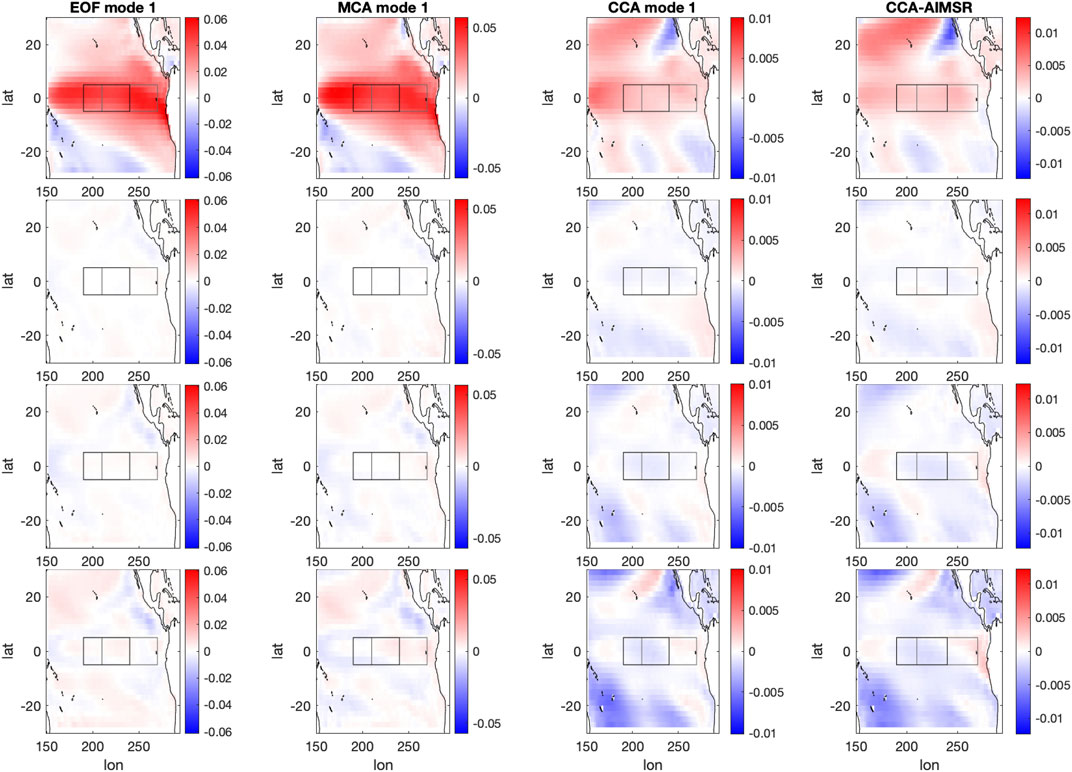
FIGURE 1. Forced change of the first modes of JJA-mean SST variability in the Equatorial Pacific. Temporal means are taken in four consecutive 50-year periods starting from 1900. The top row displays the temporal mean in the first period, and the subsequent rows display the difference with respect to that in the following periods. Leftmost column: EOF-, 2nd column: MCA-, third column: CCA first mode, last column: the only mode of CCA-AISMR. For the MCA and CCA analysis the domain on the side of the Indian monsoon is the area associated with the AISMR, as seen in Figure 2. The Niño3 and Niño3.4 boxes are marked in gray and black, respectively.

At the beginning of the simulations, EOF1, which is the most important pattern associated with ENSO variability, looks very similar to results in the literature, featuring its main “bump” in the central Pacific. Furthermore, hardly any forced change is visible in it even upon the strong RCP8.5 forcing. In comparison, Carréric et al. (2020) suggests that the maximum of the EOF1 mode shifts to the east in the CESM1-LE by showing that some center (C) mode (Takahashi et al., 2011) shifts to the east more in comparison with the westward shift of some east (E) mode¹⁴. This does not appear to be so here.

The first SST MCA mode looks practically the same when evaluated with respect to the full field and to the first three SST EOFs as seen in Supplementary Figure S2, and it is very similar to EOF1 in both cases. This suggests that MCA1 mainly reflects ENSO variability, which is further supported by the similarity in the forced changes of these patterns. We recall that these changes are minor.

In contrast to the MCA1 modes, the first CCA modes, evaluated with respect to the first 10 SST EOFs, once with the full Indian precipitation field and once with AISMR (in which case CCA1 is the only CCA mode), show considerable differences when compared to EOF1. Perhaps the main difference is a much weaker weight of the central Pacific (with more weight being concentrated to the west, perhaps because it is geographically close to India), and this might give even more importance to the observation that variability in some off-equatorial regions seems to have an opposite contribution to the teleconnection than to the main ENSO mode (EOF1). (Although, recall that the relative weights of EOFs in CCA-AISMR do not imply a similar relationship concerning the corresponding correlation coefficients.) One such region is next to South America, and another is to the east of Australia, at least at the beginning of the simulations.

The contrast in spatial features persists for the forced changes. The first CCA modes do undergo a considerable change by the late 21st century. It is even more interesting to observe this change to have a different sign in the middle of the ENSO domain (highlighted by the Niño3 and Niño3.4 boxes) compared to the sign of the minor change in the EOF1 and the MCA1 mode. On the other hand, the region to the east of Australia seems to revert its sign, finally conforming with that in EOF1.

Although each panel of Figure 1 blends 50 separate entities, the mostly monotonic emergence of the changes in consecutive rows suggests that we can see meaningful signals. Otherwise, the Supplementary Video https://youtu.be/2AVETrcfBVU shows ample year-to-year change in the form of a flickering. Given that the forcing is rather smooth and gradual (except for volcanic eruptions), this is likely just a fluctuation stemming from the error of sampling by a finite-size ensemble.

EOF2 for SST also exhibits a well-known pattern, which is practically a dipole or tripole, see Supplementary Figure S12. Its central part undergoes some degree of attenuation until 2100, except perhaps in the very middle, which can be regarded as a westward shift of one “pole” of the tripole. At the same time, areas in the north of the box gain importance. However, all changes are moderate.

CCA2, which is likely not orthogonal to CCA1, seems to be also shaped—beside EOF1—by higher-order EOFs other than EOF2 or even EOF3, which is prompted by Supplementary Figure S2. MCA2 is just in between EOF2 and CCA2, which is not surprising given that an association between MCAi and EOFi and also between MCAi and CCAi is expected. The strength of the association is determined by the regions’ own variances, on the one hand, and their interrelation, on the other.

We would like to remind though that the temporal means of the second modes are less reliable than those of the first modes, as discussed in Section 2.2, which can be seen in the Supplementary Videos https://youtu.be/EZQ7r2v7-zk and https://youtu.be/fahPv_fLgx0.

The Supplementary Figures S6, S14 suggest very similar conclusions for the first two modes in the SLP-based representations and characteristics as for SST on the side of the Pacific, except that the patterns look rather trivial for the EOFs and the MCA modes.

On the side of the IM, Figure 2 shows that the leading mode of precipitation variability (EOF1) is concentrated to the middle of the AISMR region. The MCA1 mode is somewhat different in putting more weight on the foothills of the Himalayas. This is consistent with the r map featuring the strongest correlations over land at this region; and it is epitomized by the CCA1 mode putting an overwhelming part of its weight here. CCA1 misses practically any similarity with EOF1. At the same time, the similarity of the patterns of the forced changes of the four fields shown (rows 2–4) is remarkable, even though these changes are minor over the land.

FIGURE 2

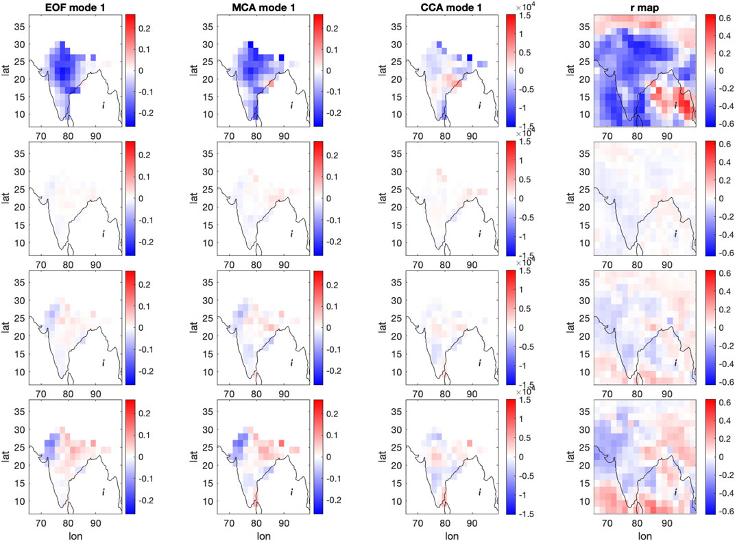
FIGURE 2. Same as Figure 1 wrt. the first three columns, but concerning the Indian summer monsoon. In the fourth column a correlation map and its changes are shown concerning the gridpoint-wise JJAS precipitation and the PC1 of the EOF1 of the SST in the box seen in Figure 1.

EOF2 for the precipitation is also very different from CCA2, see Supplementary Figure S16. EOF2 is a dipole, with an emphasis on the northeast of India but not yet at its edge. CCA2 also features important areas in the southern part of India, not coinciding with the peaks of EOF2 or EOF1. Interestingly, MCA2 is very similar to CCA2 and is thus very different from EOF2. The r map computed for the subleading mode, EOF2, of the Pacific SST field is also very different from any of these patterns. Surprisingly, it is quite similar to that computed for EOF1 (seen in Figure 2). Note that the second modes presented in Supplementary Figure S16 undergo moderate changes in time, which do not affect the conclusions of this paragraph.

Recognizing the importance of areas off the AISMR region, we repeat all computations of this section based on the precipitation field of the complete Indian box instead of the AISMR region. Surprisingly, there is hardly any alteration on the Pacific side (Supplementary Figures S5, S13). On the Indian side, as expected, CCA1 (Supplementary Figure S10) features peaks where the r maps also do, with a special emphasis on the Himalayas. Regions over the Indian Ocean lose importance with time. Interestingly, EOF1 and MCA1 (in the same figure) become similar to CCA1, although with the stronger peak appearing over the ocean (but also weakening with time).

The second modes of the complete Indian box (Supplementary Figure S18) are mainly concentrated on the sea. While CCA2 exhibits considerable similarity with the r map corresponding to EOF2 of the Pacific SST field, there are major differences with MCA2 and EOF2 in the same figure, not attenuated over time either.

So far, all joint modes presented in the analysis of the Indian patterns were based on SST on the Pacific side. Supplementary Figures S9, S11, S17, S19 illustrate that almost identical results are obtained with SLP. We thus conclude that the patterns on the Indian side are very much insensitive to the representation of variability on the Pacific side.

3.2 The Forced Evolution of Correlation Coefficients

The time evolution of the quantifiers defined in Section 2.2 is given in Figure 3 for the SST-based representations of the ENSO-side variability and applying the AISMR mask on the IM side. Concerning the affected representations involving MCA and CCA, the Mann–Kendall test statistics corresponding to the meaningful conservative r estimates are plotted for every subinterval in Figure 4, etc.

FIGURE 3

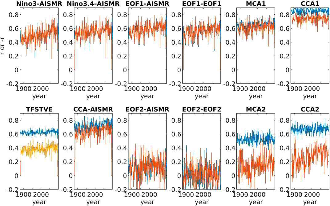
FIGURE 3. Time-evolution of the ensemble-wise correlation coefficients r associated with different representations of the ENSO-IM teleconnection or some relationship between the two domains seen in color in Figures 1, 2. In addition, in the bottom left corner we show the (square-root of the) total fraction of spatio-temporal IM variability explained, TFSTVE (Eq. 5), by PCs of the ENSO-side SMCA modes, as a further represenation of the ENSO-IM teleconnection. Blue curves show the straightforward naive estimates, and brown curves show the “conservative” estimates (see Section 2.2). In the case of TFSTVE, the yellow curve shows the estimate obtained by performing SMCA based on only 3 Equatorial Pacific SEOFs.

FIGURE 4

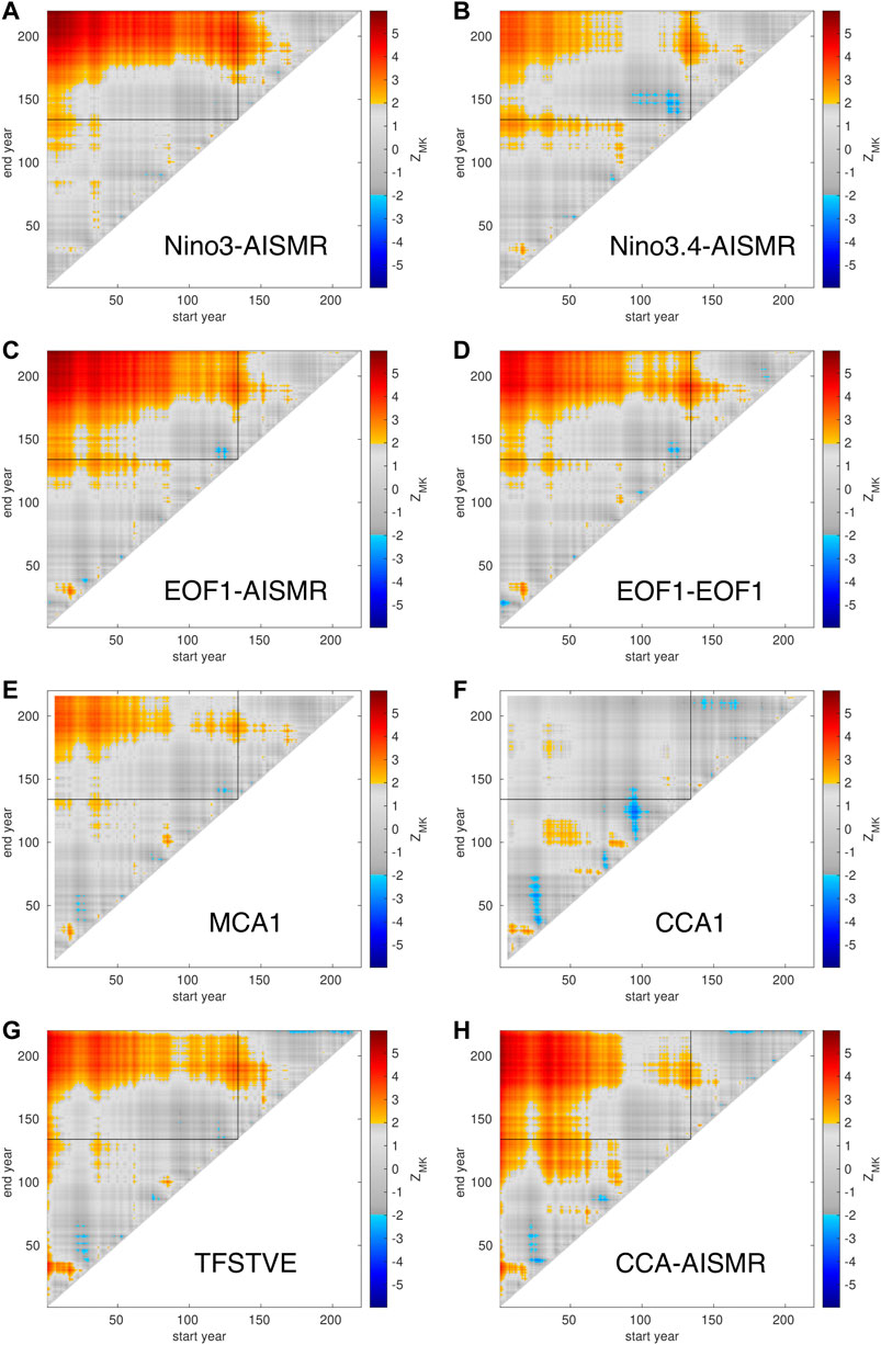
FIGURE 4. Test statistics of the Mann-Kendall test for the stationarity of (the “conservative estimates” of) $r\left(t\right)$ or $-r\left(t\right)$ (shown by the brown curves in Figure 3), depending on which of these gives an overall positive value. The diagrams correspond to panels of Figure 3 as: (A) Niño3-AISMR; (B) Niño3.4-AISMR; (C) EOF1-AISMR; (D) EOF1-EOF1; (E) MCA1; (F) CCA1; (G) TFSTVE; (H) CCA-AISMR. Red and blue shades correspond to p < 0.05, i.e., a detection of nonstationarity at that significance level.

From a technical point of view, the different estimates of r featuring a positive (blue curves) and a negative bias (brown curves) are further apart for the more erroneous MCA2 and CCA2 modes in Figure 3, as can be expected. Furthermore, even their nonstationarity is likely considerably corrupted by the positive biases. From the point of view of detectability, however, the positive bias goes with smaller statistical fluctuations. It is interesting to note that the result with positive bias does not feature much nonstationarity for either CCA1 or CCA2, while it does with CCA-AISMR. As for the result with negative bias, the nonstationarity for CCA-AISMR is in between those of CCA1 and CCA2.

A very distinct separation of the results with positive and negative bias is also seen for TFSTVE which quantifies the predictability of also the spatial variation. Furthermore, performing MCA using PC1-3 of the SST field (yellow line) is hardly different from using the full fields (brown line), which underlines that TFSTVE does represent an ENSO-IM variability. This result could perhaps be expected considering the rapid decay of the variance explained by higher-order Pacific EOFs as presented in Figure 5. Furthermore, in fact, TFSTVE is dominated overwhelmingly by MCA1, which latter on the Pacific side is in turn dominated by EOF1 (Figure 1). This is prompted by the decay of the variance explained by higher-order IM EOFs, on the one hand, and those of $r_i\left({\text{PC}}_i{\text{,PC}}_i\right)$ with the mode number i, on the other, seen also in Figure 5. In this regard we note that a further source of bias originates from taking the square of $R_m=r_m$ in Eq. 5 in conjunction with statistical errors of a near-zero $r_m$. This bias amounts to a systematic error of about 0.02, as will be indicated in Section 4.

FIGURE 5

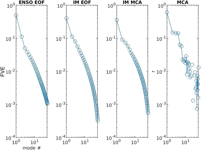
FIGURE 5. Fraction of variance explained FVE by (“raw”/“unsmoothed”) SEOF and SMCA modes. In addition, the rightmost diagram shows the “conservative” estimate of the correlation coefficients for the paired PCs of SMCA modes. Results of temporal averages for the full data span of 1880–2100 are shown in log-log diagrams.

Having said these, we conclude that TFSTVE is reasonably high to represent a strong teleconnection, and its time evolution is detected to be a long-term increase in Figure 4G. An increase is, however, not detected in shorter intervals around 1900, 2000, and in the very late 21st c.; instead, slight drops are suggested by the test statistics.

The PCs of MCA1, the leading contributor to TFSTVE, exhibit a relatively high r (MCA1 in Figure 3) with a time dependence very similar to that of TFSTVE, which carries over to the MK-test results in Figures 4E,G. r of the PCs of MCA2 is lower; in fact, it is relatively close to zero in the lower estimate (MCA2 in Figure 3). The dominant feature in its time dependence is also a long-term increase (Supplementary Figure S38C).

We recall here from the previous section that MCA modes have a similar pattern to EOFs, which may suggest that the relationship expressed by the MCA modes should be observable between the EOFs, characterizing variability of local importance, of either side. Indeed, r between the PCs of EOF1s (EOF1-EOF1 in Figure 3) is only slightly smaller than for MCA1. It undergoes a more pronounced long-term increase (Figure 4D). At the same time, r between the PCs of EOF2s (EOF2-EOF2 in Figure 3) is practically zero and is not detected to change at all (Supplementary Figure S38B). This suggests that the phenomena expressed by EOF1s are quite important for the teleconnection, but the same is not true for EOF2s.

Correlation is preserved for EOF1 and somewhat regained for EOF2 on the Pacific side when the IM side is chosen to be respresented by AISMR instead of EOFs, see EOF1-AISMR and EOF2-AISMR in Figure 3. AISMR is thus more strongly correlated with the Pacific variability than PCs of individual EOFs of the AISMR region. Temporal changes are generally also a bit more pronounced (Figure 4C; Supplementary Figure S38A).

One can then go further and take the coefficient of multiple correlation, R, of all Pacific EOFs with AISMR, which is the same as r corresponding to the single CCA-AISMR mode, a full representation of the ENSO-IM teleconnection. It is very high (see CCA-AISMR in Figure 3). It undergoes a relatively strong increase in the 20th c. with a more definite stop in the late 21st c. (Figure 4H), especially in comparison with the time evolution of TFSTVE (Figure 4G), but also with other MCA- or EOF-based characteristics (Figures 4C–E). Such differences may be related to the differences in the changes of the corresponding patterns as described in Section 3.1. Nevertheless, all main features are shared by these representations or charactersistics.

This is also true for the Niño3-AISMR and Niño3.4-AISMR representations (Figures 4A,B, both showing a high correlation in Figure 3). On the level of details, the increase of r of Niño3-AISMR extends very late to the 21st c. For r of Niño3.4-AISMR, the increase is more moderate, and a drop is undoubtedly detected after 2000, which is exceptional among the representations and characteristics discussed so far. The relative suppression of the overall increase for r of Niño3.4-AISMR may be related to the opposing changes of EOF1 and CCA-AISMR in the Niño3.4 region as discussed in Section 3.1.

CCA1 and CCA2 evaluated with the precipitation field within the AISMR region do not fit the picture outlined so far. Remember from Section 3.1 that their spatial patterns look very different from EOFs and MCA modes on the IM side and are concentrated on the very edges of the AISMR region, so that moderate importance should be associated with the corresponding results from the point of view of the teleconnection, in spite of the high correlations (CCA1 and CCA2 in Figure 3).

The shape of CCA1 and CCA2 on the IM side, together with the r maps, suggests that important areas for the teleconnection fall outside of the AISMR region and prompts to evaluate modes of spatiotemporal variability in the complete Indian box. As mentioned in Section 3.1, this brings modes of the same order similar to each other and to the r maps of the Pacific EOFs, reveals the importance of the bulk of the Himalayas and of oceanic areas, and a loss of this importance with time. This importance loss might imply that characteristics of the teleconnection might strengthen more when they are based solely on the AISMR region rather than the complete box.

We do observe in Supplementary Figures S26, S34 that results for TFSTVE, the MCA modes and the paired EOFs are very similar for the complete box as for the AISMR region except that the signal of strengthening is much weaker (and turns to a pronounced weakening for EOF2-EOF2). At the same time, CCA1 and CCA2 now exhibit strengthening (with the previously described intermittent periods), even stronger than the other characteristics. However, for characteristics for which AISMR is replaced by the mean box precipitation (BOXSR), the correlation becomes unreasonably low. These characteristics do not deserve further analysis and illustrate that applying appropriate techniques to select IM-related precipitation within the box is essential.

Using SLP instead of SST in a suitable subset of the Pacific box does not yield any difference that would be worth mentioning (Figure 6; Supplementary Figures S25, S27, S33, S35, S39, S41, except for SOI and box-SOI). This means that SLP reflects the same phenomenology as SST in the respective domains. The results with SOI and box-SOI are similar to the rest, and differences in the details are not possible to interpret without extending the currently used domain to the west.

FIGURE 6

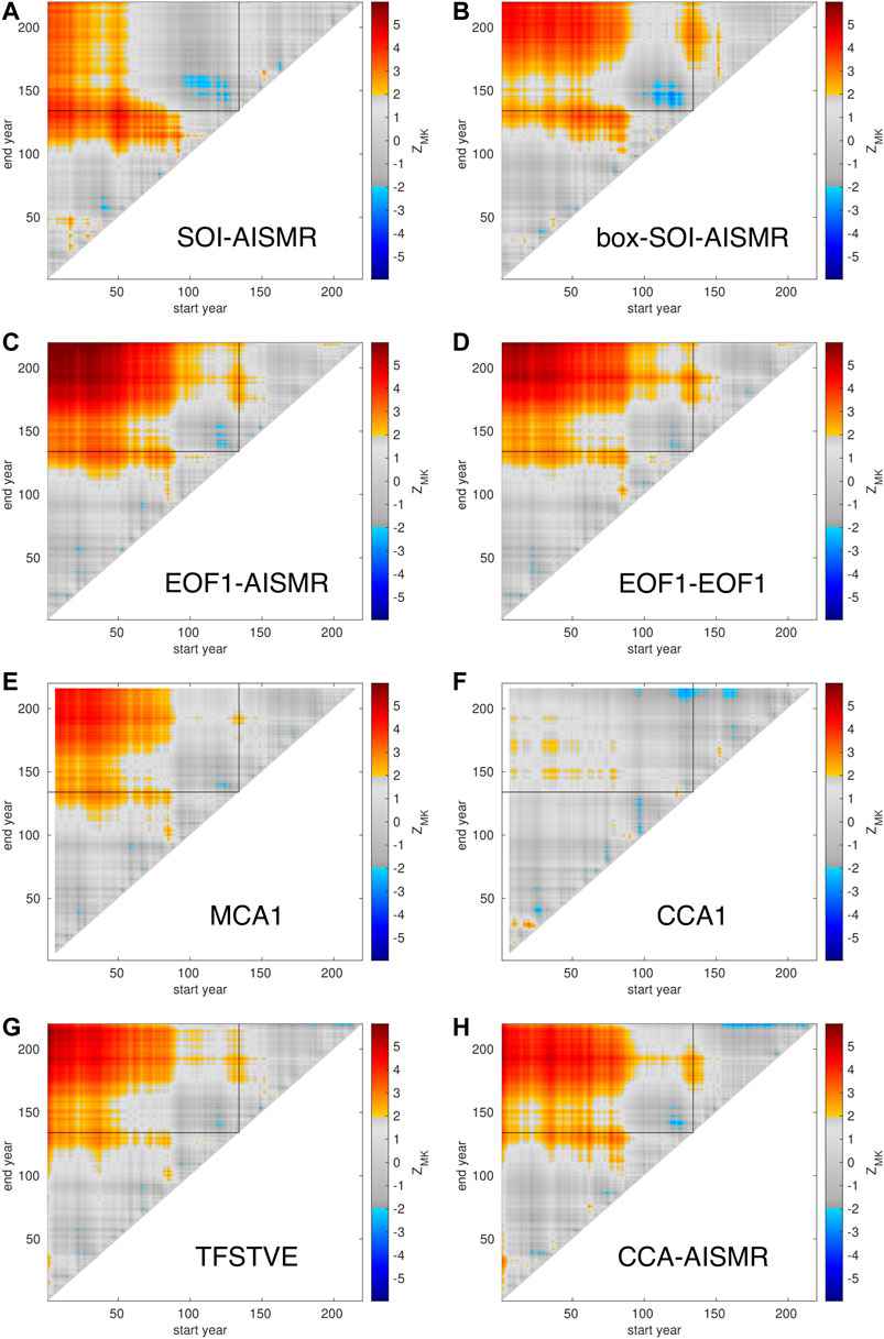
FIGURE 6. Same as Figure 4 but the ENSO side is characterized based on the SLP.

3.3 The Drivers of Changes in Correlation Coefficients

Having established the observable changes, we can now ask about their drivers in terms of the linear regression model as introduced in Section 2.3. We emphasize again that attribution in the case of characteristics involving MCA and CCA is in general not possible. Furthermore, we do not perform statistical tests here regarding these drivers. Therefore, the attribution of a change in r to different factors is not rigorous but rather tentative.

Figure 7 suggests that ENSO-side variability, ${\sigma }_{\text{Φ}}$, first stagnates then increases with time in the early 21st c. irrespective of which dominant mode is taken. This seems to be followed by an equally fast decrease starting from the mid 21st c., with seemingly all of the gain lost by the end of the century in view of Niño3 and PC1. The decrease is a bit more moderate with Niño3.4, which should contribute to the result that ENSO variability can dominate changes in the correlation coefficient by the late 21st c. as seen in Figure 8B. Although, no doubt another reason is that in this representation the coupling a increases less and ${\sigma }_{\xi }$ increases more than for other characteristics. Beside the decrease of ${\sigma }_{\text{Φ}}$ in the second half of the 21st c., a continued increase of $a/{\sigma }_{\xi }$ might still make r continue to increase. However, $a/{\sigma }_{\xi }$ might also experience a nonmonotonicity, although likely starting to decrease later than ${\sigma }_{\text{Φ}}$. If that happens, clearly $r\left(t\right)$ would be also nonmonotonic. However, this is not detected (Figure 6), perhaps because of the shortness of the time period when this happens. Another important nontriviality in the time evolution of $a/{\sigma }_{\xi }$ is a drop at the turn of the 20th–21st centuries. This drop is related to a drop in the time evolution of a and serves as a possible explanation for the drop in the correlation coefficient at the same time. It turns out from Figure 7 that both a and ${\sigma }_{\xi }$ typically undergo a considerable increase otherwise, with a “winning,” but only slightly.

FIGURE 7

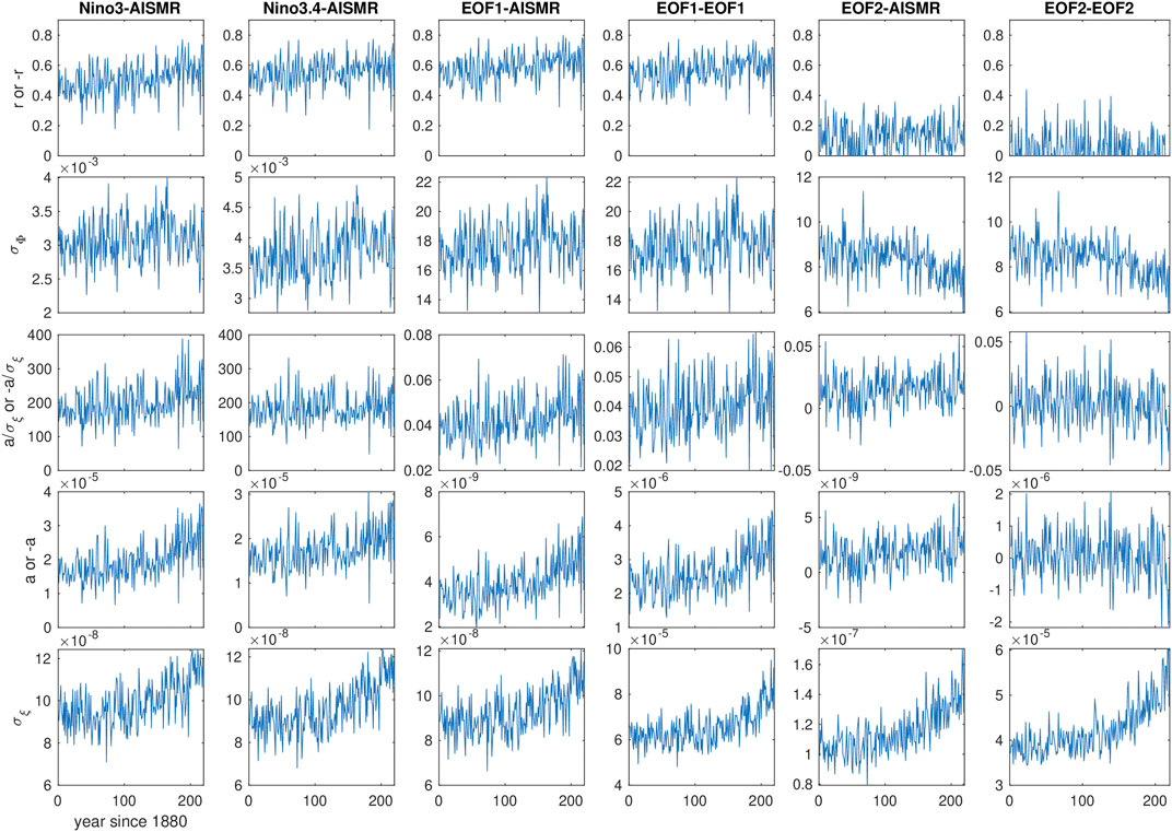
FIGURE 7. The forced evolution of correlation coefficients $r\left(t\right)$ and the drivers of change; see Section 2.3. The different columns correspond to different representations of the relationship between the variability in the regions of ENSO and the IM. For columns 1–3 and 5 the IM is represented by the average monsoon rain AISMR. Columns 1–4 concern the dominant modes of variability, and columns 5–6 concern the next-to-dominant modes of variability.

FIGURE 8

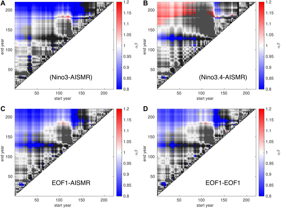
FIGURE 8. Relative importance of ${\sigma }_{\text{Φ}}$ versus $a/{\sigma }_{\xi }$ to the change of $r\left(t\right)$. The diagrams correspond to those of Figure 4 showing the Mann–Kendall test statistics for $r\left(t\right)$. Color is applied only where $r\left(t\right)$ changes significantly. The color saturates where $\alpha \beta$ is outside of the range indicated in the colorbars.

Making use of the SLP mostly agrees with the findings obtained with the SST, see Figures 6, 9. The only but important exception is a decreasing ENSO-side variability in view of PC1. We note that the same domain as used for the SST is not suited for the SLP: the corresponding principal modes (whether SEOFs, SMCA and SCCA modes) are unrelated to the essence of the ENSO phenomenon, as a concentration of the high-amplitude areas on the edges of the domain indicates (Bódai et al., 2020a).

FIGURE 9

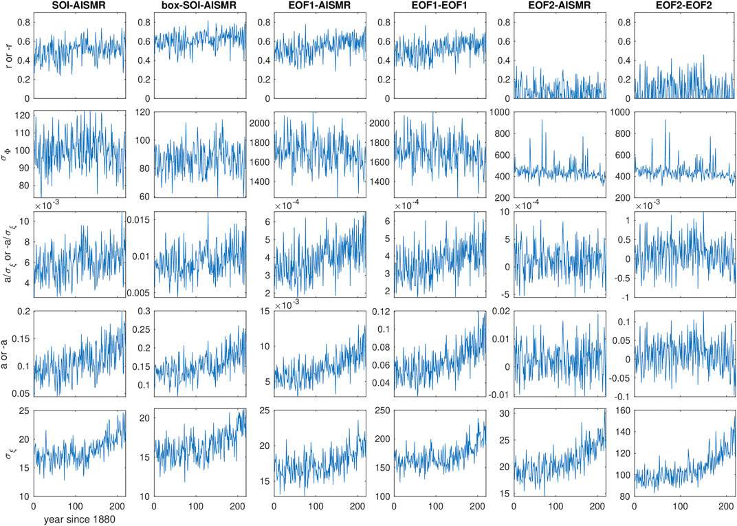
FIGURE 9. Same as Figure 7 but the ENSO side is characterized based on the SLP.

Although second modes were found to be relatively unimportant for the teleconnection, there seems to be considerable nonstationarity in ${\sigma }_{\text{Φ}}$ for EOF2, which might still have an impact on an other important teleconnection representation, CCA-AISMR.

4 Comparison of the MPI-GE to Observations and Reanalysis

Results and conclusion that derive from a large ensemble apply only to the model that generated the data. However, the ultimate enquiry pertains to the actual Earth system, and, in that regard, one should perform some comparison of the model with observations. Clearly, it has its limitations given that the observational record corresponds to a single realization, and, so, it provides proportionally less information about the system. In (Bódai et al., 2020b) we compared long-term means and trends of the SST fields and precipitation in South Asia, as well as temporal correlation coefficients pertaining to areal means like e.g. the AISMR and Niño3. Our conclusion was, however, that it is not possible to detect nonstationarity from single realisations. In terms of spatial modes of variability and associated correlations, it is likewise doubtful to be able to establish the forced response from observational data. What we can compare here are modes and correlations that are in a way overall “representative of a time period.”

Calculations are carried out with respect to temporal variability, not only for observations, but also for each member of the ensemble, so as to make a comparison meaningful. In turn, the different realisations for the model will provide some statistics for the finite-size temporal estimates. As proper anomalies cannot be obtained for observations, we instead feed the calculations with data that represent “high-frequency variability.” It is obtained by subtracting a low-frequency component from every data point, which is approximately a 21 years moving window mean. We use the same method as in (Bódai et al., 2020b), applying a Savitzky–Golay filter of order 3 to the running window means. We obtain conservative estimates e.g. for r associated with PCs belonging to modes by parting the data into two consecutive periods of equal length, computing the modes from the first part, and computing PCs by projecting the fields given by the second part onto those modes.

The data representing observations are obtained from the 20th century CERA 20C reanalysis product (Laloyaux et al., 2018) for Pacific SST, and the CRU PRE v4.03 gridded precipitation data (Harris, 2019a; Harris, 2019b) for the Indian summer monsoon rain. We analyze the time period of 1901–2010. Precipitation variables are not available for CERA 20C, hence, we can make a comparison with the model only with respect to the representation where the AISMR domain is used. This is not a problem from the point of view that only land areas have a practical relevance. The precipitation data of the 20th Century Reanalysis V2 data (Compo et al., 2011) is not so faithful to reality; it does not reproduce the AISMR time series (Parthasarathy et al., 1994) well, and yields only an r(Niño3, AISMR) = –0.2.

The results for the SST principal modes are displayed in Figure 10. The ensemble means of the temporal modes in the top row are hard to distinguish from the temporal means of the snapshot modes as seen in Figure 1. In the second row the ensemble standard deviations reveal that the sampling error is much bigger to do with the CCA compared to the MCA and EOF. The observational EOF1 is more concentrated on the Eastern Equatorial Pacific, or, at least, it does not feature a second peak in the Western Equatorial Pacific like the model does. The weight of the observational MCA1 mode is somewhat shifted to the west wrt. EOF1. The observational CCA1 and CCA-AISMR modes are similar to one another, just like those of the models, but the respective observational modes are much less similar to the model modes as compared to EOF1 and MCA1. The observational CCA1 and CCA-AISMR modes are concentrated to the middle of the Equatorial Pacific while the model modes on the westernmost of the Equatorial Pacific and even on off-equatorial areas. Yet, the associated correlation coefficients match very closely (Figure 11F).

FIGURE 10

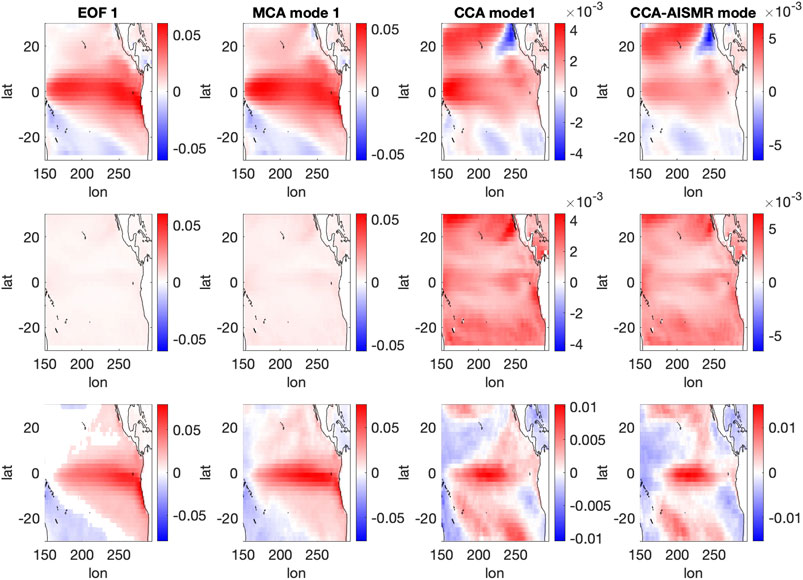
FIGURE 10. Comparison of principal SST modes obtained by temporal EOF analysis, MCA, CCA (the columns corresponding to those of Figure 1) between the MPI-ESM (top row) and observation (bottom row). In the middle row the ensemble-wise standard deviations are shown in the same color range as the modes themselves.

FIGURE 11

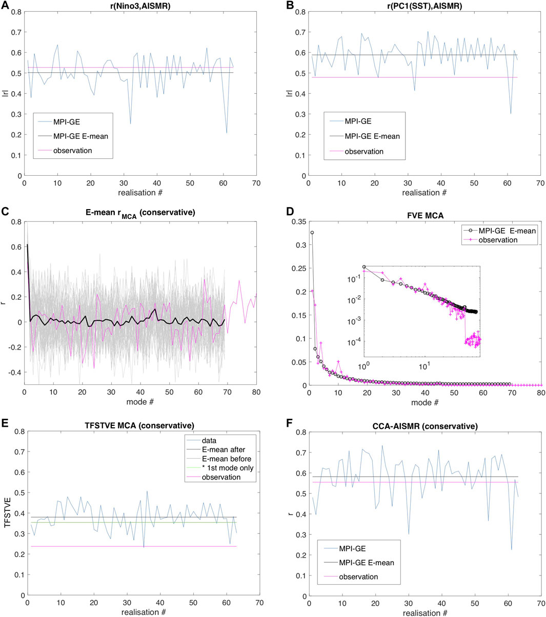
FIGURE 11. Comparison of temporal correlation coefficients r(A-C,F), FVE (D), TFSTVE (E), between the MPI-ESM (blue, black, gray, green curves) and observation (magenta curve) for various representations of the ENSO-IM teleconnection. Panel (E) indicates that the systematic error for the conservative estimate of TFSTVE (brown curve) in Figure 3 is about 0.02.

As for the IM side, the modes are shown in Figure 12. Again, regarding the model, the resemblance of the ensemble means of the temporal modes in the top row and the temporal means of the snapshot modes as seen in Figure 2 is uncanny. It is rather surprising that the CCA1 modes on the IM side match rather well between observation and model. Otherwise, so do the r maps and the MCA1 modes match rather well. The observational EOF1, however, does not appear to closely resemble the observational MCA1 mode, unlike for the model, which might have only to do with the fact that the model does not resolve the very wet climatology over the Western Ghats. The fact that the observational MCA1 mode does not have a strong weight over the Western Ghats despite the high resolution should have to do with the weak correlations with PC1 of the Equatorial Pacific SST in this area, as shown by the r maps.

FIGURE 12

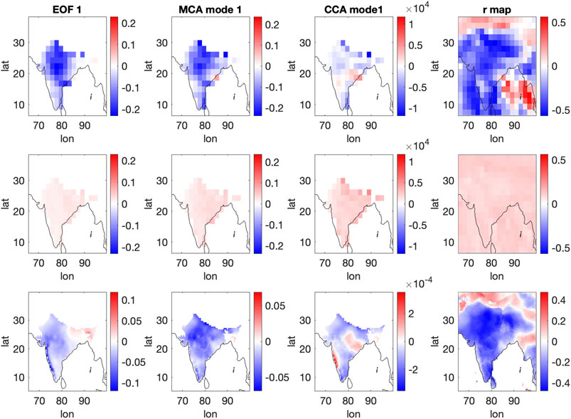
FIGURE 12. Same as Figure 10, but for the Indian summer monsoon precipitation (the columns corresponding to those of Figure 2).

Some of these observations apply also to the second modes. It is particularly surprising how the observational and model CCA2 modes both on the Pacific (Supplementary Figure S42) and IM side (Supplementary Figure S43) resemble one another, even despite the large sampling fluctuations as shown in the middle rows.

As for the correlation coefficients r and TFSTVE, seen in Figure 11, the estimate from observations is always smaller, except for the Ninõ3-AISMR representation [in panel (A)]. It is not clear how this exception could be explained by the restriction of the observational EOF1 to the east (Figure 10, bottom left), if it could be at all. It is the CCA-AISMR representation (F) that yields the largest (conservative estimate of) r also for observations, very slightly below the figure for the model. In contrast, the TFSTVE (E) is considerably smaller for observations, which is prompted by both r (C) and FVE (D) being smaller for the observational MCA1 mode. Nevertheless, these diagrams suggest that this can be just a statistical fluctuation of the single observational realization. Note also that r for the higher-order MCA modes is practically zero; that is, only MCA1 contributes to the TFSTVE.

We emphasize once again that the above comparison cannot confirm confidence that the MPI-GE correctly features a strengthening ENSO-IM teleconnection. Neither can it undermine the confidence thanks to the fairly close match in most aspects, the observational results falling seemingly within the ensemble-wise variation of the MPI-GE estimates.

5 Nonergodicity

Whenever the forced change is nonlinear, whether due to a nonlinear progression of the forcing or a nonlinear response characteristic, an estimation of the momentary ensemble-mean climatology by a temporal mean in a finite window should be biased (Drótos et al., 2016). That is, the ensemble mean of the temporal mean would not be equal to the ensemble mean itself (say, at the middle of the time window), which is termed nonergodicity. Higher-order statistics should be biased even in the unlikely case that the forced change of the ensemble mean is linear and the internal variability would not feature a forced change. The linear Pearson correlation coefficient is no exception, i.e., its time-based evaluation (the traditional choice) will be biased even if the ensemble means of the correlated quantities exhibit a temporally linear forced response. Notwithstanding, a linear time evolution of the Pearson correlation coefficient $r\left(t\right)$ itself may lead to a vanishing bias, and this is what we will elaborate on in this section.

In fact, $r\left(t\right)$ clearly features a nonlinear change in various representations and characteristics of the ENSO-IM teleconnection and related quantifiers in the MPI-GE, whether it is a monotonic but degressive change (represented by a concave graph) or a nonmonotonic one, as seen in Figures 4, 6, 7, 9. However, the evaluation of the bias or the degree of nonergodicity is not straightforward in this case since the “signal-to-noize ratio” is rather poor thanks to the relatively small ensemble size. Nevertheless, we can attempt to at least detect the presence of nonergodicity by performing a statistical test. The quantity of the so-called test statistics can in turn serve as some quantifier of the degree of nonergodicity.

To the end of constructing a suitable test, we observe that the Fisher transform $\widehat{z}=\text{arctanh}\left(\widehat{r}\right)$ ($\widehat{r}$ distinguishes the finite-N sample estimate of r) provides approximately normally distributed independent identically distributed random variables (wrt. the different years) with a standard deviation $\approx 1/\sqrt{N-3}$ for large enough N and any true value r of the correlation coefficient.¹⁵ The same applies, of course, to the finite-τ-window sample correlation coefficient $r_{\tau }$ when $\text{Φ}\left(t\right)$, $\text{Ψ}\left(t\right)$ are not auto-correlated and their ensemble means and standard deviations remain constant in time. In such a case, the only reason that the expectation

$\langle {\left({\widehat{z}}_{\tau }-z\right)}^2\rangle (7)$

at any time does not match the theoretical value ${\left(\tau -3\right)}^{-1}$ is the existence of a bias:

$\langle {\widehat{z}}_{\tau }\rangle \ne z\text{,}(8)$

i.e., nonergodicity.

We have four issues to consider. First, z is not available because of the finite N ensemble size. Therefore, we cannot evaluate nonergodicity at any time (every year). Instead, we can consider nonergodicity overall in an interval of length T calculating

$v={\displaystyle \sum _{t=1}^T{\displaystyle \sum _{n=1}^N{\left({\widehat{z}}_{\tau ,t,n}-{\widehat{z}}_t\right)}^2}}\text{.}(9)$

Second, had ${\widehat{z}}_{\tau }$ and $\widehat{z}$ in the above been computed from combinations from the same sample of size $T=N$ (without repetition), Cochran’s theorem (Cochran, 1934) would dictate that $cv$ (where c is an appropriate constant factor) would be distributed according to a ${\chi }^2$-distribution. This would allow for calculating the p-value in the usual way by evaluating the ${\chi }^2$-distribution at the level given by the calculated test statistics. However, our setting is somewhat different T = N, which might not be possible to tackle analytically. Nevertheless, one can sample the test statistics and, therefore, determine its quantiles to arbitrary precision. We have performed this sampling simply by generating sample correlation realisations by generating realisations of correlated random variables X and Y, where $Y=aX+\xi$, and X and $\xi$ are normally distributed independent random variables. This is a further assumption for the nature of our variables, from which deviations certainly exist but which are presumably moderate enough to have a secondary effect for the results. Note that the moving-window temporal correlation coefficient ${\widehat{r}}_{\tau ,t}$ is calculated upon pregenerating $x_t$ and $y_t$, $t=1,\dots ,T$. We have checked that $cv$ does seem to follow a ${\chi }^2$-distribution even in our setting, but we do not utilize it.

Third, $\text{Φ}$ is in fact auto-correlated, regardless of the choice to represent ENSO-related variability. As a simple test, we took X to be governed by an auto-regressive process of order 1, $X_{t+1}=\varphi X_t+{\xi }_t$, such that the lag-1 autocorrelation is 0.3, and we have found only little shift in the distribution of v wrt. its standard deviation. We also took this value of 0.3, and calculated the 0.95 quantile of v, obtaining about 670 using the parameters $T=220$, $\tau =31$, $N=63$; while it is 667 with a serially uncorrelated $X_t$.

As a fourth issue, there might be a low-frequency influence on the teleconnection, say, via a time-dependent a (Gershunov and Barnett, 1998; Torrence and Webster, 1999; Krishnamurthy and Goswami, 2000; Krishnamurthy and Krishnamurthy, 2014; Watanabe and Yamazaki, 2014). This should increase the width of the distribution of the sample temporal correlation coefficient, i.e., it should be larger than $1/\sqrt{N-3}$. We tested the effect of this by introducing an additive perturbation, $a_t=a_0+\delta a_t$, where $\delta a_t$ is modeled again as an AR(1) process, setting $\varphi =0.8$ and such a noise strength that $\text{std}\left[\delta a_t\right]=0.05$. With this the 0.95 quantile is 674; that is, the effect is rather small. This corroborates well with the findings of (Gershunov et al., 2001; Yun and Timmermann, 2018), namely, that even if there was a low-frequency modulation of the ENSO-IM teleconnection strength, it would be too weak to detect from century-long observations. The cancellation effect described by Krishnamurthy and Goswami (2000) may be an alternative view of this.

Turning to our application, the test statistics is found to be 756 for the ENSO-IM teleconnection representation given by the Niño3-AISMR pair. That is, it is well above the 0.95 quantile, corresponding to a minuscule p-value, so that the hypothesis of ergodicity can be rejected with extremely high confidence. We also evaluate the test statistics corresponding to the global correlation maps seen in Supplementary Figure S1. The result of this can be presented as a global map, too (Figure 13), in which a contour for the 0.95 quantile, 670, encloses regions where ergodicity can be rejected at the usual significance level of 0.05. We can see such regions not just in the tropics or in the Equatorial Pacific, but all over the world. Nevertheless, the highest levels of bias/nonergodicity is indeed found at the center of ENSO variability and elsewhere in the Equatorial Pacific.

FIGURE 13

FIGURE 13. Test statistics of our ad hoc test of nonergodicity regarding the Pearson correlation coefficient. The contours mark the 0.95 quantile. Here, ENSO is represented by PC1 of EOF1.

We note that even if $r\left(t\right)$ changes linearly, or not at all, there could be a trivial source of the bias, namely, a changing ensemble mean or standard deviation of $\text{Φ}$ or $\text{Ψ}$. We redo the calculation of the test statistics in order to exclude the former trivial source. In particular, we subtract the respective ensemble-mean time series from the $\text{Φ}$ and $\text{Ψ}$ time series, separately for each ensemble member, before calculating the temporal correlation coefficient ${\widehat{r}}_{\tau }$. The result (Supplementary Figure S44) is hardly distinguishable from the original one (Figure 13) with respect to the patterns, only the values of v are slightly off. That is, in this case the change of the mean state hardly contributes to the bias. As mentioned, the forced change of the standard deviation can also be a source of bias. We believe that, just as the ensemble-mean change, this is also a negligible effect, considering especially that in windows of $\tau =30$ yr the changes of the ${\sigma }_{\text{Φ}}$ time series seem unlikely to be detectable in Figures 7, 9. For this reason, nonergodicity should robustly imply the nonlinearity of $r\left(t\right)$.

6 Discussion and Conclusion

We have re-examined the forced response of the ENSO-Indian monsoon (IM) teleconnection as conveyed by the MPI-GE data. One main increment taken by the new analysis is the consideration of spatial aspects of any forced change. This was achieved by determining empirical orthogonal functions (EOFs) and modes of Maximum Covariance Analysis (MCA) and Canonical Correlation Analysis (CCA), and considering various characteristics and representations of the teleconnection defined through these tools. Beyond individual correlation coefficients, we defined the total fraction of the spatio-temporal IM variability explained (TFSTVE) by the Pacific variability, and interpreted results in the spirit of the coefficient of multiple correlation, R. We found that both TFSTVE and R are dominated by the first-order modes, both wrt. their magnitude and forced changes. Characterizing different aspects of the relationship between the variability of the two regions allowed us to build a robust picture of forced changes.

We have found almost all characteristics and representations to convey a picture of a strengthening teleconnection in terms of a statistical test, confirming earlier findings. One or two slight drops around the turn of the 20th–21st centuries have also been detected, and the increase in strength has been found to slow down in the late-21st c. The latter aspect is more prominent when spatial variability is taken into account on a wider region around India, including the Himalayas and surrounding oceanic areas. We have found indications that using such a region may be more suited to analyzing and understanding the teleconnection between ENSO and the IM, but aspects specific to the traditional observational product of all-Indian summer monsoon rainfall (AISMR) may be underrepresented and overlooked in this way.

The late-21st c. slowdown mostly has to do with a curious nonmonotonicity in the change of the ENSO variability: in most representations of ENSO variability, about midway in the 21st c. rather suddenly it starts to decline. In terms of a linear regression model that can be associated with evaluating the (linear) Pearson correlation coefficient, the typically increasing regression coefficient—which can be viewed as an ENSO-IM coupling strength—also plays a strong role. Although the model’s noise strength undergoes a similar increase, which has an opposing role, the change of the coupling is found to dominate. The latter turns out to be the central piece of the robust or consistent picture of the strengthening ENSO-IM teleconnection. We conjecture that the temporary drop or drops in the teleconnection strength at the turn of the 20th–21st centuries are also related to corresponding changes in the coupling strength.

We leave it for future work to attribute these features to physical effects. In any case, the change of both the coupling and noise strength should involve both thermodynamic and dynamic factors.

Some differences between different characterstics and representations are due to changes in the relevant spatial patterns. The most interesting finding is that the pattern of maximal ENSO variability and that of maximal correlation with the IM precipitation undergo opposing trends in the middle of the ENSO domain: the middle becomes more important for ENSO itself, while it loses importance for the teleconnection. On the side of the IM, the AISMR region gains relative importance for local variability and even more for the teleconnection with ENSO.

It is essential to note that based on observations the ENSO-IM teleconnection appears to have weakened since about 1980 (Kumar et al., 1999; Bódai et al., 2020b). In (Bódai et al., 2020b) we argued that several reasons could be responsible for this mismatch. Among them one is that the MPI-ESM associated with the MPI-GE is not consistent with the observations of the 20th c. Indian Ocean (IO) warming and IM precipitation decline: in terms of the long-term trend, the ranges of simulated realisations, wrt. both the IO temperature and ISMR, do not contain the observations as respective single realisations–by far [see Figures 12, 13 of (Bódai et al., 2020b)]. See (Aneesh and Sijikumar, 2018), for example, for the role of the IO warming regarding the decline of ISMR, concerning La Niña years, in particular. However, it is a question yet to be answered if the decline of precipitation does actually translate into a weakening of the ENSO-IM teleconnection in the precise sense of a forced change.

Another possibility for the reason for the said mismatch was posited in (Bódai et al., 2020b) to be the very considerable fluctuations of temporal correlation coefficients—the larger in magnitude the shorter the time window—even under stationary unforced conditions, and even without decadal variability of the correlated signals. Evaluating temporal correlations is troubled by further problems when there is a forced change, namely, that 1) when the forced change is nonlinear, the temporal correlations are biased (Section 5), and that 2) the forced signal is not known, and, therefore, the anomalies that are meant to be correlated cannot even be constructed. A detrending, say, removing a linear slope in a time window, does not seem to be a good fix, as even under stationary conditions one would find spurious trends due merely to internal variability, and, so, we would remove a signal that should not be removed.

When an ensemble is available, concerning a single model at least, the biases to do with point 1) above can be detected and, to a certain extent, quantified. We have developed an ad hoc statistical test to do just that, and applied it to the ENSO-IM teleconnection as well as the relationship of global precipitation and ENSO. We have found many regions of the world where a bias could be detected. The reasons for the nonlinearities that such biases imply can be manifold, not only driven by the nonlinearity of the change of ENSO variability, and it should be carefully examined in the future.

Our methodology indeed ensures that the detected biases imply nonlinearity (i.e., not only nonlinearity implies biases, but also the other way round). In our context of the historical and scenario change of ENSO-precipitation teleconnections, robust nonlinearity has been found. Given that nonlinearity implies (presupposes) a forced change, we turn out to have on hand a statistical test for the nonstationarity of teleconnections (linear correlations). This can be seen to complement the Mann-Kendall test (in the special case of the nonstationarity of the correlation coefficient), because the latter takes the alternative hypothesis of a monotonic change, while our test includes nonmonotonic changes too.

Data Availability Statement

The data generated and analysed for this study are available upon reasonable request. For reproducing purposes, one can make use of the MPI-GE data available at https://esgf-data.dkrz.de/projects/mpi-ge/, as suggested in Section 2. Observational/reanalysis data sets analysed in Section 4 are available at the webpages whose URL's are included in the bibliographic entries.

Author Contributions

TB developed any new code, including those implementing SMCA and SCCA, carried out all the numerical analyses and created all the figures for the paper. GD and subsequently TB originated the ideas of SMCA and SCCA, respectively. TB proved the equivalence of the correlation coefficient of CCA with a scalar target and the coefficient of multiple correlation. TB proposed the breaking down of the change of the correlation coefficients into three constituents according to the linear regression model. TB devised the statistical test for nonergodicity of correlations motivated by Axel Timmermann’s enquiry. GD, J-YL, E-SC suggested to calculate the differences as e.g., in Figure 1; and to evaluate the relative importance of ENSO variability as seen in Figure 8 developed and implemented by TB. TB and GD lead the interpretation of results and the writing of the manuscript. K-JH, J-YL, E-SC contributed to the manuscript.

Funding

TB was supported by the Institute for Basic Science (IBS), under IBS-R028-D1. G.D. acknowledges financial support from the Spanish State Research Agency through the María de Maeztu Program for Units of Excellence in R&D under grant no. MDM-2017-0711, from the National Research, Development and Innovation Office (NKFIH, Hungary) under grant nos. K125171 and FK-124256, and from the European Social Fund through the fellowship no. PD/020/2018 under the postdoctoral program of the Government of the Balearic Islands (CAIB, Spain). Support for the Twentieth Century Reanalysis Project dataset is provided by the U.S. Department of Energy, Office of Science Innovative and Novel Computational Impact on Theory and Experiment (DOE INCITE) program, and Office of Biological and Environmental Research (BER), by the National Oceanic and Atmospheric Administration Climate Program Office, and by the National Oceanic and Atmospheric Administration Climate Program Office, and by the NOAA Physical Sciences Laboratory.

Conflict of Interest

The authors declare that the research was conducted in the absence of any commercial or financial relationships that could be construed as a potential conflict of interest.

Acknowledgments

TB thanks Tímea Haszpra, Malte Stuecker, Kyung-Sook Yun for useful discussions regarding applying spatial weighting according to Baldwin et al. (2009), an appropriate domain for modal analysis using the SLP, using gridded observational precipitation data (CRU PRE) only but not unreliable reanalysis data, respectively, and Axel Timmermann for his interest in nonergodicity including a discussion on whether nonergodicity implies the nonlinear change of correlations and vice versa. GD thanks Claudia E. Wieners for useful discussions about the relationship between ENSO and the total variability of the Equatorial Pacific. TB thanks Keith Rodgers for informing him about the volume of Variations that includes (Haszpra et al., 2020b). GD is thankful to B. Stevens, T. Mauritsen, Y. Takano, and N. Maher for providing access to the output of the MPI-ESM ensembles. 20th Century Reanalysis V2 data provided by the NOAA/OAR/ESRL PSL, Boulder, Colorado, United States, from their Web site at https://psl.noaa.gov/. Free access to the CRU PRE data and the CERA 20C reanalysis product is gratefully acknowledged. The preprint of this paper (Bódai et al., 2020a) can be found at https://arxiv.org/abs/2009.02155. The authors acknowledge the constructive comments by the two reviewers, one of whom prompted the definition of TFSTVE.

Supplementary Material

The Supplementary Material for this article can be found online at: https://www.frontiersin.org/articles/10.3389/feart.2020.599785/full#supplementary-material.

Footnotes

¹It is, therefore, instructive to study a multimodel ensemble of SMILEs.

²We do not regard the co-evolution of the ensemble means of e.g., Niño3 and the Indian summer monsoon rain to be part of the teleconnection, unlike Pandey et al. (2020), as these responses could be largely unrelated. Yet, using an infinite ensemble, the rank correlation coefficient with respect to the temporal variability, i.e., evolution, of the ensemble means is trivially 1. The prediction or projection of the Indian summer monsoon rain does not even need to rely on the Equatorial Pacific SST, but could be just facilitated by e.g., some extrapolation of the observed response of its own. That is, if there was reason to believe that we have a reliable estimate of the forced response.

³We emphasize that the bias that defines “nonergodicity” is based on the ideal ensemble mean, not a sample mean for a finite-size ensemble.

⁴Such a feature is absent in the CESM1-LE (Haszpra et al., 2020a).

⁵The case of the standard deviation, a statistic of basic interest giving a primary representation of internal variability, is already nontrivial, as nonstationarity would imply heteroscedasticity, in which case the reliable detection of nonstationarity is not straightforward. Assuming homoscedasticity wrongly, the estimates of standard errors could be either negatively or positively biased, and, therefore, a type II error can be made: not rejecting stationarity at a certain confidence level when the process is actually nonstationary.

⁶The quotation marks are used because the concept of a “snapshot” makes the best sense concerning a time-continuous evolution, whereas here we consider the discrete-time annual progression of a seasonal mean.

⁷Ensemble-wise EOFs, SEOFs, were used earlier in the context of probabilistic ensemble forecasting in e.g., (Zheng et al., 2013; Zheng et al., 2017; Zheng et al., 2019), in which case the concern was certainly not the forced response.

⁸It is also common to redefine PCs to be normalized and EOFs to be multiplied by the corresponding standard deviations.

⁹Although, the rationale behind defining simple indices is such that we want to work with a simple-to-compute quantity (e.g., an areal average or difference between two locations) that correlates very strongly with the dominant variability in terms of EOFs, which latter can be seen to represent a more natural method of decomposing the variability of a field.

¹⁰If the same wider box is used with the SLP as with the SST, the “weight” of the EOF1 is concentrated on parts of the perimeter of the box. Despite the dissimilarity of the EOF1s with the SLP in the two different boxes, the time dependence of the corresponding correlation coefficients r(PC1,AISMR) are actually very similar.

¹¹Strictly speaking, each mode should be tested if it can be distinguished from noise and if it features characteristics associated with ENSO.

¹²As for the MCA, maximizing the unexplained covariance implies that the PCs are uncorrelated as reflected by the SVD decomposition.

¹³SST mask mode 1: https://youtu.be/2AVETrcfBVU

SST mask mode 2: https://youtu.be/EZQ7r2v7-zk

SST box mode 1: https://youtu.be/C62BKGVDQvQ

SST box mode 2: https://youtu.be/QgLQCbS3ZRU

SLP mask mode 1: https://youtu.be/HbxJjOz1RUA

SLP mask mode 2: https://youtu.be/fahPv_fLgx0

SLP box mode 1: https://youtu.be/PQHv7B8B2sw.

SLP box mode 2: https://youtu.be/74_ltkeOiqg.

¹⁴situation is not shown conclusively in (Haszpra et al., 2020a) because only three snapshots are shown belonging to single years, and it is not clear how much statistical error is associated with them, leaving an uncertainty about the locations of the peaks.

¹⁵This approximation assumes the correlated variables to follow a Gaussian distribution, but non-Gaussianity has been checked to have a farly negligible effect for some basic ENSO-quantifiers and AISMR in (Bódai et al., 2020b).

References

Aneesh, S., and Sijikumar, S. (2018). Changes in the La Niña teleconnection to the Indian summer monsoon during recent period. J. Atmos. Sol. Terr. Phys. 167, 74–79. doi:10.1016/j.jastp.2017.11.009

CrossRef Full Text | Google Scholar

Baldwin, M. P., Stephenson, D. B., and Jolliffe, I. T. (2009). Spatial weighting and iterative projection methods for EOFs. J. Clim. 22, 234–243. doi:10.1175/2008JCLI2147.1

CrossRef Full Text | Google Scholar

Björnsson, H., and Venegas, S. A. (1997). A manual for EOF and SVD analyses of climatic data. Tech. rep. 97 (1), 112–134.

Google Scholar

Bódai, T., Drótos, G., Ha, K.-J., Lee, J.-Y., Haszpra, T., and Chung, E.-S. (2020a). Nonlinear forced change and nonergodicity: the case of ENSO-Indian monsoon and global precipitation teleconnections arXiv.2009.02155. Atmos. Oceanic Phys. Available at: https://arxiv.org/abs/2009.02155

Google Scholar

Bódai, T., Drótos, G., Herein, M., Lunkeit, F., and Lucarini, V. (2020b). The forced response of the El niño–southern oscillation–Indian monsoon teleconnection in ensembles of earth system models. J. Clim. 33, 2163–2182. doi:10.1175/JCLI-D-19-0341.1

CrossRef Full Text | Google Scholar

Bódai, T., and Tél, T. (2012). Annual variability in a conceptual climate model: snapshot attractors, hysteresis in extreme events, and climate sensitivity. Chaos: An Interdisciplinary J. Nonlinear Sci. 22, 023110. doi:10.1063/1.3697984

CrossRef Full Text | Google Scholar

Carréric, A., Dewitte, B., Cai, W., Capotondi, A., Takahashi, K., Yeh, S.-W., et al. (2020). Change in strong Eastern Pacific El Niño events dynamics in the warming climate. Clim. Dynam. 54, 901–918. doi:10.1007/s00382-019-05036-0

CrossRef Full Text | Google Scholar

Cochran, W. G. (1934). The distribution of quadratic forms in a normal system, with applications to the analysis of covariance. Math. Proc. Camb. Phil. Soc. 30, 178–191. doi:10.1017/S0305004100016595

CrossRef Full Text | Google Scholar

Compo, G. P., Whitaker, J. S., Sardeshmukh, P. D., Matsui, N., Allan, R. J., Yin, X., et al. (2011). The Twentieth century reanalysis Project. Q. J. R. Meteorol. Soc. 137, 1–28. doi:10.1002/qj.776

CrossRef Full Text | Google Scholar

Drótos, G., Bódai, T., and Tél, T. (2015). Probabilistic concepts in a changing climate: a snapshot attractor picture. J. Clim. 28, 3275–3288. doi:10.1175/JCLI-D-14-00459.1

CrossRef Full Text | Google Scholar

Drótos, G., Bódai, T., and Tél, T. (2016). Quantifying nonergodicity in nonautonomous dissipative dynamical systems: an application to climate change. Phys. Rev. E 94, 022214. doi:10.1103/PhysRevE.94.022214

PubMed Abstract | CrossRef Full Text | Google Scholar

Drótos, G., Bódai, T., and Tél, T. (2017). On the importance of the convergence to climate attractors. Eur. Phys. J. Spec. Top. 226, 2031–2038. doi:10.1140/epjst/e2017-70045-7

CrossRef Full Text | Google Scholar

Fisher, R. A. (1915). Frequency distribution of the values of the correlation coefficient in samples from an indefinitely large population. Biometrika 10, 507–521.

CrossRef Full Text | Google Scholar

Franzke, C. L. E. (2014). Nonlinear climate change. Nat. Clim. Change 4, 423–424. doi:10.1038/nclimate2245

CrossRef Full Text | Google Scholar

Gershunov, A., and Barnett, T. P. (1998). Interdecadal modulation of ENSO teleconnections. Bull. Am. Meteorol. Soc. 79, 2715–2726. doi:10.1175/1520-0477(1998)079<2715:IMOET>2.0.CO;2

CrossRef Full Text | Google Scholar

Gershunov, A., Schneider, N., and Barnett, T. (2001). Low-frequency modulation of the ENSO–Indian monsoon rainfall relationship: signal or noise? J. Clim. 14, 2486–2492. doi:10.1175/1520-0442(2001)014<2486:LFMOTE>2.0.CO;2

CrossRef Full Text | Google Scholar

Ghil, M., and Lucarini, V. (2020). The physics of climate variability and climate change. Rev. Mod. Phys. 92, 035002. doi:10.1103/RevModPhys.92.035002

CrossRef Full Text | Google Scholar

Härdle, W., and Simar, L. (2007). Canonical correlation analysis. Berlin, Heidelberg: Springer Berlin Heidelberg, 321–330. doi:10.1007/978-3-540-72244-1_14

CrossRef Full Text

Harris, I. (2019a). [Dataset]: CRUTS v4.03 data variables: PRE. https://crudata.uea.ac.uk/cru/data/hrg/cru_ts_4.03/cruts.1905011326.Ωv4.03/pre/

Google Scholar

Harris, I. (2019b). [Dataset]: Release notes for CRU TS v4.03. https://crudata.uea.ac.uk/cru/data/Ωhrg/cru_ts_4.03/Release_Notes_CRU_TS4.03.txt

Google Scholar

Haszpra, T., Herein, M., and Bódai, T. (2020a). Investigating ENSO and its teleconnections under climate change in an ensemble view—a new perspective. Earth Syst Dyn. 11, 267–280. doi:10.5194/esd-11-267-2020

CrossRef Full Text | Google Scholar

Haszpra, T., Topál, D., and Herein, M. (2020b). “Detecting forced changes in internal variability using Large Ensembles: on the use of methods based on the “snapshot view.” New research on climate variability and change using initial-condition Large Ensembles. Variations. Editors C. Deser, and K. Rodgers (Washington: UCAR), Vol. 18, 36–43.

Google Scholar

Haszpra, T., Topál, D., and Herein, M. (2020c). On the time evolution of the arctic oscillation and related wintertime phenomena under different forcing scenarios in an ensemble approach. J. Clim. 33, 3107–3124. doi:10.1175/JCLI-D-19-0004.1

CrossRef Full Text | Google Scholar

Heffernan, P. M. (1997). Unbiased estimation of central moments by using U-statistics. J. Roy. Stat. Soc. B 59, 861–863.

CrossRef Full Text | Google Scholar

Herein, M., Márfy, J., Drótos, G., and Tél, T. (2016). Probabilistic concepts in intermediate-complexity climate models: a snapshot attractor picture. J. Clim. 29, 259–272. doi:10.1175/JCLI-D-15-0353.1

CrossRef Full Text | Google Scholar

Kay, J. E., Deser, C., Phillips, A., Mai, A., Hannay, C., Strand, G., et al. (2015). The community Earth system model (CESM) large ensemble project: a community resource for studying climate change in the presence of internal climate variability. Bull. Am. Meteorol. Soc. 96, 1333–1349. doi:10.1175/BAMS-D-13-00255.1

CrossRef Full Text | Google Scholar

Kim, B.-H., and Ha, K.-J. (2015). Observed changes of global and western Pacific precipitation associated with global warming SST mode and mega-ENSO SST mode. Clim. Dynam. 45, 3067–3075. doi:10.1007/s00382-015-2524-2

CrossRef Full Text | Google Scholar

Krishnamurthy, L., and Krishnamurthy, V. (2014). Influence of PDO on South Asian summer monsoon and monsoon–ENSO relation. Clim. Dynam. 42, 2397–2410. doi:10.1007/s00382-013-1856-z

CrossRef Full Text | Google Scholar

Krishnamurthy, V., and Goswami, B. N. (2000). Indian monsoon–ENSO relationship on interdecadal timescale. J. Clim. 13, 579–595. doi:10.1175/1520-0442(2000)013<0579:IMEROI>2.0.CO;2

CrossRef Full Text | Google Scholar

Kumar, K. K., Rajagopalan, B., and Cane, M. A. (1999). On the weakening relationship between the Indian monsoon and ENSO. Science 284, 2156–2159. doi:10.1126/science.284.5423.2156

PubMed Abstract | CrossRef Full Text | Google Scholar

Laloyaux, P., de Boisseson, E., Balmaseda, M., Bidlot, J. R., Broennimann, S., Buizza, R., et al. (2018). CERA-20C: a coupled reanalysis of the twentieth century. J. Adv. Model. Earth Sys. 10 (5), 1172–1195. doi:10.1029/2018MS001273

CrossRef Full Text | Google Scholar

Maher, N., Milinski, S., Suarez-Gutierrez, L., Botzet, M., Dobrynin, M., Kornblueh, L., et al. (2019). The Max Planck Institute Grand ensemble: enabling the exploration of climate system variability. J. Adv. Model. Earth Syst. 11, 2050–2069. doi:10.1029/2019MS001639

CrossRef Full Text | Google Scholar

Mann, H. B. (1945). Nonparametric tests against trend. Econometrica 13, 245–259.

CrossRef Full Text | Google Scholar

Meinshausen, M., Smith, S. J., Calvin, K., Daniel, J. S., Kainuma, M. L. T., Lamarque, J.-F., et al. (2011). The RCP greenhouse gas concentrations and their extensions from 1765 to 2300. Climatic Change 109, 213. doi:10.1007/s10584-011-0156-z

CrossRef Full Text | Google Scholar

Mishra, V., Smoliak, B. V., Lettenmaier, D. P., and Wallace, J. M. (2012). A prominent pattern of year-to-year variability in Indian Summer Monsoon Rainfall. Proc. Natl. Acad. Sci. Unit. States Am. 109, 7213–7217. doi:10.1073/pnas.1119150109

CrossRef Full Text | Google Scholar

North, G. R., Bell, T. L., Cahalan, R. F., and Moeng, F. J. (1982). Sampling errors in the estimation of empirical orthogonal functions. Mon. Weather Rev. 110, 699–706. doi:10.1175/1520-0493(1982)110<0699:SEITEO>2.0.CO;2

CrossRef Full Text | Google Scholar

Pandey, P., Dwivedi, S., Goswami, B. N., and Kucharski, F. (2020). A new perspective on ENSO-Indian summer monsoon rainfall relationship in a warming environment. Clim. Dynam. 55, 3307–3326. doi:10.1007/s00382-020-05452-7

CrossRef Full Text | Google Scholar

Parthasarathy, B., Munot, A. A., and Kothawale, D. R. (1994). All-India monthly and seasonal rainfall series: 1871–1993. Theor. Appl. Climatol. 49, 217–224. doi:10.1007/BF00867461

CrossRef Full Text | Google Scholar

Power, S. B., and Delage, F. P. D. (2018). El Niño–Southern Oscillation and associated climatic conditions around the world during the latter half of the twenty-first century. J. Clim. 31, 6189–6207. doi:10.1175/JCLI-D-18-0138.1

CrossRef Full Text | Google Scholar

Quadrelli, R., Bretherton, C. S., and Wallace, J. M. (2005). On sampling errors in empirical orthogonal functions. J. Clim. 18, 3704–3710. doi:10.1175/JCLI3500.1

CrossRef Full Text | Google Scholar

Santer, B. D., Fyfe, J. C., Solomon, S., Painter, J. F., Bonfils, C., Pallotta, G., et al. (2019). Quantifying stochastic uncertainty in detection time of human-caused climate signals. Proc. Natl. Acad. Sci. Unit. States Am. 116, 19821–19827. doi:10.1073/pnas.1904586116

CrossRef Full Text | Google Scholar

Storch, H. V., and Zwiers, F. W. (1999). Statistical analysis in climate research. Cambridge, United Kingdom: Cambridge University Press. doi:10.1017/CBO9780511612336

CrossRef Full Text

Takahashi, K., Montecinos, A., Goubanova, K., and Dewitte, B. (2011). ENSO regimes: reinterpreting the canonical and modoki El Niño. Geophys. Res. Lett. 38. doi:10.1029/2011GL047364

CrossRef Full Text | Google Scholar

Tél, T., Bódai, T., Drótos, G., Haszpra, T., Herein, M., Kaszás, B., et al. (2019). The theory of parallel climate realizations. J. Stat. Phys. 179 (5–6), 1496–1530. doi:10.1007/s10955-019-02445-7

CrossRef Full Text | Google Scholar

Timmermann, A. (1999). Detecting the nonstationary response of ENSO to greenhouse warming. J. Atmos. Sci. 56, 2313–2325. doi:10.1175/1520-0469(1999)056<2313:DTNROE>2.0.CO;2

CrossRef Full Text | Google Scholar

Topál, D., Ding, Q., Mitchell, J., Baxter, I., Herein, M., Haszpra, T., et al. (2020). An internal atmospheric process determining summertime arctic sea ice melting in the next three decades: lessons learned from five large ensembles and multiple CMIP5 climate simulations. J. Clim. 33, 7431–7454. doi:10.1175/JCLI-D-19-0803.1

CrossRef Full Text | Google Scholar

Torrence, C., and Webster, P. J. (1999). Interdecadal changes in the ENSO–monsoon system. J. Clim. 12, 2679–2690. doi:10.1175/1520-0442(1999)012<2679:ICITEM>2.0.CO;2

CrossRef Full Text | Google Scholar

Vega-Westhoff, B., and Sriver, R. L. (2017). Analysis of ENSO’s response to unforced variability and anthropogenic forcing using CESM. Sci. Rep. 7, 18047. doi:10.1038/s41598-017-18459-8

PubMed Abstract | CrossRef Full Text | Google Scholar

Wang, B. (2006). The Asian Monsoon. Berlin, Germany: Springer-Verlag. doi:10.1007/3-540-37722-0

CrossRef Full Text

Wang, B., Xiang, B., Li, J., Webster, P. J., Rajeevan, M. N., Liu, J., et al. (2015). Rethinking Indian monsoon rainfall prediction in the context of recent global warming. Nat. Commun. 6, 7154. doi:10.1038/ncomms8154

PubMed Abstract | CrossRef Full Text | Google Scholar

Watanabe, T., and Yamazaki, K. (2014). Decadal-scale variation of South Asian summer monsoon onset and its relationship with the pacific decadal oscillation. J. Clim. 27, 5163–5173. doi:10.1175/JCLI-D-13-00541.1

CrossRef Full Text | Google Scholar

Yettella, V., Weiss, J. B., Kay, J. E., and Pendergrass, A. G. (2018). An ensemble covariance framework for quantifying forced climate variability and its time of emergence. J. Clim. 31, 4117–4133. doi:10.1175/JCLI-D-17-0719.1

CrossRef Full Text | Google Scholar

Yun, K.-S., and Timmermann, A. (2018). Decadal monsoon-ENSO relationships reexamined. Geophys. Res. Lett. 45, 2014–2021. doi:10.1002/2017GL076912

CrossRef Full Text | Google Scholar

Zheng, M., Chang, E. K. M., and Colle, B. A. (2013). Ensemble sensitivity tools for assessing extratropical cyclone intensity and track predictability. Weather Forecast. 28, 1133–1156. doi:10.1175/WAF-D-12-00132.1

CrossRef Full Text | Google Scholar

Zheng, M., Chang, E. K. M., Colle, B. A., Luo, Y., and Zhu, Y. (2017). Applying fuzzy clustering to a multimodel ensemble for U.S. East coast winter storms: scenario identification and forecast verification. Weather Forecast. 32, 881–903. doi:10.1175/WAF-D-16-0112.1

CrossRef Full Text | Google Scholar

Zheng, M., Chang, E. K. M., and Colle, B. A. (2019). Evaluating U.S. East coast winter storms in a multimodel ensemble using EOF and clustering approaches. Mon. Weather Rev. 147, 1967–1987. doi:10.1175/MWR-D-18-0052.1

CrossRef Full Text | Google Scholar