South Atlantic Anomaly Areal Extent as a Possible Indicator of Geomagnetic Jerks in the Satellite Era

Introduction

The secular variation of the core geomagnetic field is generally characterized by smooth variations in time. However, since the end of the 1970s with the works of Courtillot et al. (1978) and Malin et al. (1983), the geomagnetic community has been interested in the occurrence of abrupt changes, not globally simultaneous (Brown et al., 2013), observed in the trend of the first derivative of the field elements, mostly Y (East) component, recorded at geomagnetic observatories, called geomagnetic jerks.

There exist many techniques to detect geomagnetic jerks, from spectral decomposition methods such as wavelet analysis (e.g., Alexandrescu et al., 1996) and Slepian functions expansions (Kim and von Frese, 2013) to nonlinear techniques such as nonlinear forecasting approach (Qamili et al., 2013). However, up to date, the most used technique to find out geomagnetic jerks is that based on the direct identification of V-shape in the secular variation of one geomagnetic field component (X, Y, Z) registered in ground geomagnetic observatories, mainly in the East component (Y) because it is the least affected by external fields at midlatitudes (Pinheiro et al., 2011; Torta et al., 2015). Following this approach, Pinheiro et al. (2011) used annual means of the geomagnetic components X, Y, and Z coming from geomagnetic observatories distributed around the world to estimate the occurrence time of the 1969, 1978, 1991, and 1999 geomagnetic jerks. Brown et al. (2013) improved the methodology applied by Pinheiro et al. (2011) using monthly means of the three geomagnetic components in more than 100 observatories, and then histograms with periods of most frequent jerk activity from 1957 to 2008 were estimated. Later, Torta et al. (2015) estimated the 2007, 2011, and 2014 jerks occurrence times following an analogous procedure to that described in Pinheiro et al. (2011) but using only the geomagnetic component Y. They used between six and four geomagnetic observatories to estimate the occurrence times of the most recent geomagnetic jerks.

In the last 2 decades, five well-defined geomagnetic jerks have been widely accepted by scientific community (see, e.g., Brown et al., 2013; Torta et al., 2015). These most recent geomagnetic jerks, reported in 1999 (Mandea and Macmillan, 2000), 2003 (Olsen and Mandea, 2008), 2007 (Olsen et al., 2009; Chulliat et al., 2010), 2011 (Chulliat and Maus, 2014), and 2014 (Torta et al., 2015), have been found to occur at a regular rate of one every 3–4 years. This suggests that they are caused by a quasi-oscillatory phenomenon within the outer core. New high-resolution satellite data provided by the last satellite missions, such as Swarm from European Space Agency (ESA) (Friis-Christensen et al., 2006), have improved the geomagnetic field models and, in turn, the knowledge of the dynamic processes occurring close to the outer core. As a result, one can obtain reliable estimations of the secular acceleration (SA) of the geomagnetic field and its time variations at the Core-Mantle Boundary (CMB). However, it is important to mention that the SA is less constrained for short wavelengths, which increases the difficulty to study rapid fluctuations at these scales (Gillet, 2019). Chulliat et al. (2010) and Chulliat and Maus (2014) observed that the geomagnetic jerks happened between two peaks of SA at the CMB and applied a Principal Component Analysis (Chulliat and Maus, 2014) to establish the principal modes of variability of the SA associated with the occurrence of the geomagnetic jerks. They found maxima and minima lobes of the SA located on the equatorial region in South Atlantic Ocean and South America and in the Indian Ocean. In a very recent work, Kloss and Finlay (2019) found that in these same sectors magnetic field acceleration pulses are produced by alternating prominent bursts of nonzonal azimuthal flow acceleration in the equatorial region beneath the CMB. Moreover, they found alternated sign of the acceleration at some regions that, when associated with large spatial scale structures, could cause geomagnetic jerks at the Earth’s surface.

By using global geomagnetic field models based on paleomagnetic data, Terra-Nova et al. (2016) observed that the reversed flux patches (RFPs) present at the CMB, that is, regions with an opposite polarity to that expected for an axial dipole, for the last three millennia, were mostly located in the Southern Hemisphere, especially in the South Atlantic and Indian regions.

In the last decades, the presence of two RFPs located beneath South America and South Africa from 1840 has been observed (Gubbins et al., 2006), although recent studies (Tarduno et al., 2015; Campuzano et al., 2019) point out that they could be even older (950 AD or earlier). These RFPs are commonly associated with the internal origin of the South Atlantic Anomaly (SAA) (e.g., Hulot et al., 2002; Olson and Amit, 2006; Laj and Kissel, 2015; Pavón-Carrasco and De Santis, 2016; Terra-Nova et al., 2017), a region with anomalously low values of geomagnetic field intensity at the Earth’s surface. In Figure 1, the present situation of the intensity and the radial component (Br) of the geomagnetic field at the surface and CMB, respectively, are shown. The SAA is also related to the continuous decreasing of the dipole moment of the geomagnetic field in the last 150 years (Finlay et al., 2016a; Terra-Nova et al., 2017). This has motivated some authors to study this feature as a possible precursor of a next geomagnetic transition, such as an excursion or a reversal (De Santis et al., 2013; Laj and Kissel, 2015; Pavón-Carrasco and De Santis, 2016).

FIGURE 1

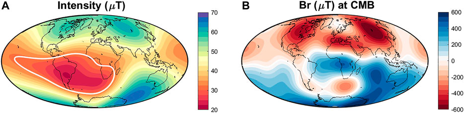
FIGURE 1. Geomagnetic field on January 1, 2020. (A) Intensity at the surface and (B) radial component (Br) of the geomagnetic field at the CMB on January 1, 2020, from CHAOS-7.2 model (Finlay et al., 2020). The white line in (A) marks the contour line of 32,000 nT to highlight the area of the SAA defined following De Santis et al. (2012). In (B) the two RFPs related to the presence of the SAA at the surface are observed in red colors in the Southern Hemisphere. We use CHAOS-7.2 model until degree 13 to calculate the intensity at the surface and until degree six for Br at the CMB.

In the search for understanding geomagnetic jerks, an important element is to investigate possible correlations between these events and some other geophysical phenomena (see Mandea et al., 2010 for a review on some of the up-to-date suggested links). In the present paper, we suggest that the minima of the acceleration of the areal extent of SAA could be a reliable indicator of the occurrence of geomagnetic jerks, being able to register all of the well-defined geomagnetic jerks for the last 2 decades.

In the next sections, we describe the methods, together with the most important results, and then provide a discussion about the dynamic processes at the CMB that could be involved in this link and the possible identification of future geomagnetic jerks occurrence from this result.

Methods and Results

This study has been carried out using the CHAOS-7.2 model, the release of the CHAOS-7 model (Finlay et al., 2020) that uses the Swarm preliminary baseline 0603 data up to the end of March 2020 and ground observatory data as available in February 2020. The Swarm satellite mission (Olsen and Haagmans, 2006 and references therein) was launched by ESA in November 2013. This mission, based on a constellation of three identical satellites (Alpha, Bravo, and Charlie), provides high quality measurements of the geomagnetic field in three different orbital planes, with Alpha and Charlie flying almost in parallel and Bravo orbiting alone at a higher altitude. These data, along with those given by other previous satellite missions (Cryosat-2, CHAMP, SAC-C, and Ørsted) and the global network of magnetic observatories at ground level, provide the possibility of obtaining high-resolution time-dependent geomagnetic field models such as the CHAOS-7 model and later releases.

According to Domingos et al. (2017), there are several ways to define the SAA position and, depending on the choice, the shape and evolution of the SAA could be slightly different. An operative and simple way to define the SAA in terms of its areal extent is to consider the area within the contour of 32,000 nT at the Earth’s surface following De Santis et al. (2012). We calculate its area (S) monthly from January 1998 to March 2020 using the CHAOS-7.2 model until maximum spherical harmonic degree 13 that corresponds to the main geomagnetic field. As can be observed in Figure 2A, the areal extent of the SAA has been continuously growing during the entire period, from 9.49 ∙ 10⁷ km² to 10.47 ∙ 10⁷ km². In order to evaluate in detail the evolution of this increase, we also study the rate of change of the areal extent of the SAA by applying the first and second derivatives to the previously calculated area (S) (Figures 2B–C). For the first derivative estimation, $\dot{S}$, we use the finite differences between successive times, t_i and t_i+1, from January 1998 to March 2020, centered in the mean time, using

${\dot{S}}_{t_{i+\frac{1}{2}}}=\frac{S_{t_{i+1}}-S_{t_i}}{\left(t_{i+1}-t_i\right)},(1)$

with t_i+1/2 = t_i + 3 months and t_i+1 = t_i + 6 months, in order to provide smooth changes.

FIGURE 2

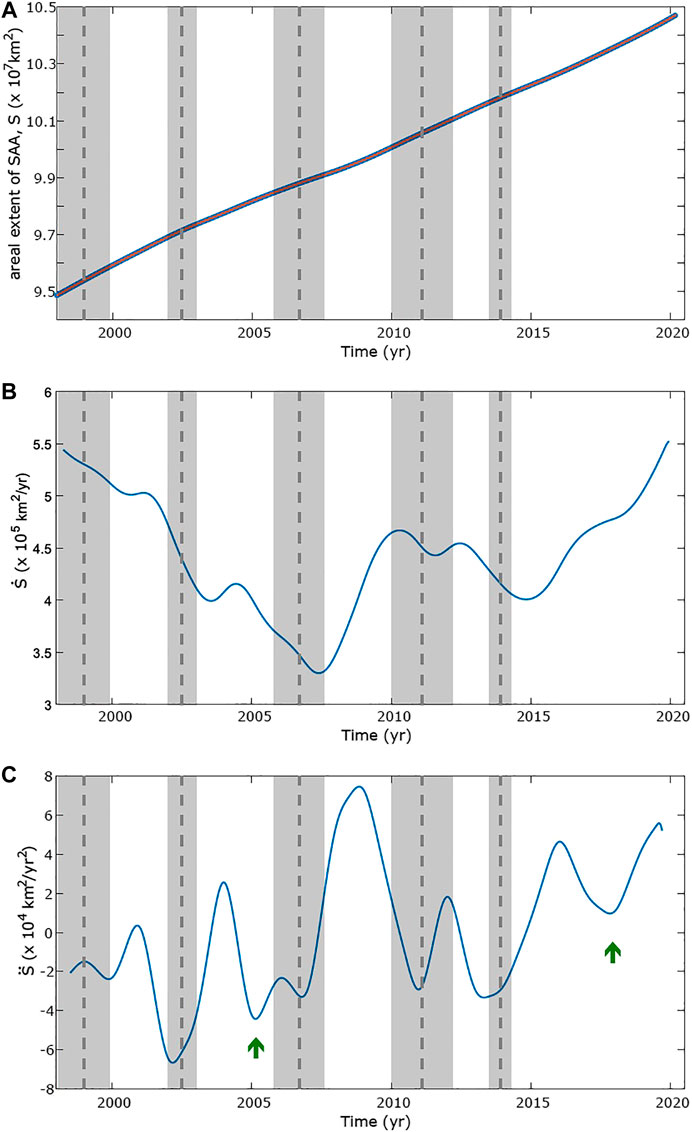
FIGURE 2. South Atlantic Anomaly evolution. (A) Evolution S, (B) first derivative S ̇, and (C) second derivative S ̈ of the areal extent of the SAA for the last 2 decades calculated from CHAOS-7.2 model monthly from January 1998 to March 2020. The fit of the areal extent of the SAA by using cubic splines is plotted in orange in (A). In dashed vertical gray lines, the mean occurrence times of the well-defined geomagnetic jerks for the last 2 decades are marked. Shaded bands mark the uncertainty of the occurrence times given by one standard deviation. With green arrows some interesting features are indicated (see Discussion in the main text for more details).

For the second derivative, $\stackrel{\cdot \cdot }{S}$, we use the finite differences method of second order following Tozzi et al. (2009), with t_i+1 = t_i + 6 months and t_i−1 = t_i−6 months for the same period.

Prior to the estimation of these derivatives, we smooth the areal extent of the SAA series by fitting the data using a cubic splines basis with knot points every year from 1998 to 2020.2 in order to avoid subsequent mathematical artifacts from the derivatives (orange line in Figure 2A).

As expected, the $\dot{S}$ values are positive (Figure 2B); that is, the areal extent of the SAA is increasing in the analyzed time interval with an average rate of 4.4 ∙ 10⁵ km²/yr. In Figure 2C it is observed that this increase of the SAA is not continuously accelerated (see also Pavón-Carrasco and De Santis, 2016), alternating periods of accelerations (beginning –1999.0, 1999.9–2000.9, 2002.2–2004.0, 2005.1–2006.1, 2006.8–2008.8, 2011.0–2012.0, 2013.3–2016.0, and 2017.8–2019.6) and decelerations (1999.0–1999.9, 2000.9–2002.2, 2004.0–2005.1, 2006.1–2006.8, 2008.8–2011.0, 2012.0–2013.3, 2016.0–2017.8, and 2019.6– end). The time intervals when the $\stackrel{\cdot \cdot }{S}$ reaches positive values (2000.7–2001.1, 2003.6–2004.4, 2007.4–2010.3, 2011.6–2012.5, 2014.8– end) are characterized by longer displacements of the areal extent of the SAA. These intervals present a duration from 1 to 3 years, being the longest period of positive $\stackrel{\cdot \cdot }{S}$, that is, the maximum increase of areal extent of the SAA for the last 2 decades, between 2007 and 2010. Actually, the longest period with positive $\stackrel{\cdot \cdot }{S}$ would be from 2014.8 up to now, but this result must be considered carefully because it could be affected by edge problems of the CHAOS-7.2 model. These edge problems could also be present at the beginning of the model, the borders being the periods most subject to change. On the other hand, in the minima of $\stackrel{\cdot \cdot }{S}$ (1999.9, 2002.2, 2005.1, 2006.8, 2011.0, 2013.3, and 2017.8) the areal extent of the SAA is slowing down its advancement.

The comparison between the occurrence of these minima and the well-defined geomagnetic jerks reported during the last 2 decades is shown in Figure 2C. Since the geomagnetic jerks are not registered simultaneously in all geomagnetic observatories, we can find differences between observations of the same jerk in two different observatories even of around two years (e.g., Mandea et al., 2010). The shaded bands in Figure 2 give information about this fact. For representation of shaded bands, we have taken the occurrence times from previously published works. In detail (the following occurrence times for the different jerks are summarized in Supplementary Table S1):

- The 1999 geomagnetic jerk occurrence time: occurrence dates of the 1999 geomagnetic jerk were given in Supplementary Table A4 by Pinheiro et al. (2011). They are 54 occurrence dates calculated from the annual means of the geomagnetic components X, Y, and Z in 42 observatories. The mean (and standard deviation) of these 54 occurrence dates provides the value of 1999.0 (±0.9) plotted in Figure 2C.

- The 2003 geomagnetic jerk occurrence time: the 2003 geomagnetic jerk is identified by a relative peak in number of global jerk identifications between 2002 and 2003 (see Figure 15 in Brown et al., 2013). This interval can be rewritten as 2002.5 (±0.5) and plotted in Figure 2C.

- The 2007, 2011, and 2014 geomagnetic jerks occurrence times: they were obtained by Torta et al. (2015) using the method proposed by Pinheiro et al. (2011) on Y component. The 2007 geomagnetic jerk occurrence time was calculated in five different geomagnetic observatories providing five occurrence dates. The 2011 geomagnetic jerk occurrence time was calculated from four different observatories and the 2014 one from six different observatories. The mean (and standard deviation) of the occurrence times are 2006.7 (±0.9), 2011.1 (±1.1), and 2013.9 (±0.4), respectively. These values are plotted in Figure 2C. It is important to note that these observatories are not evenly distributed geographically. More space and time extended studies of magnetic observatories could result in more accurate estimations of the occurrence times of these jerks.

As we can observe, the minima of the acceleration ($\stackrel{\cdot \cdot }{S}$) of the areal extent of the SAA (Figure 2C) coincide quite well with the geomagnetic jerks occurrence for the last 2 decades.

To reinforce the obtained link, we have performed several tests to verify the independence of the results with 1) the model used to calculate the SAA areal extent and 2) the SAA definition. For the first objective, we have compared our results with those given by a previous version of the CHAOS model, the CHAOS-6-x8 (Finlay et al., 2016b), that used a previous version of Swarm data (v.0505) up to the end of August 2018 and ground observatory data available at the same epoch, and with the GRIMM-3 model (Lesur et al., 2011). This last model is mainly an improvement of GRIMM-2 (Lesur et al., 2010), which was generated from CHAMP satellite data and observatory hourly means, and it is valid from January 2001 to July 2009. As we can see in Supplementary Figures S1–S2 of the Supplementary Material, the minima of the acceleration of the areal extent of SAA are detected in similar times as when the CHAOS-7.2 is used (Figure 2C). The main differences are found in the earlier times but within the uncertainty shown by shaded bands.

For the second objective, we have changed the definition of the SAA using 1) a different contour line of 28,000 nT, which corresponds to the lowest value of geomagnetic field intensity registered over the interest area in 1840 AD, computed using the historical geomagnetic field model GUFM1 (Jackson et al., 2000), and 2) the new measure to characterize the SAA area proposed by Amit et al. (2020). The results (Supplementary Figures S3–S4 in the Supplementary Material) are in agreement with those obtained previously. The most notable discrepancies are seen using the definition proposed by Amit et al. (2020) in the second derivative of the SAA areal extent, especially in the recent times, where the edge effects could be more significant by the effect of the smoothing of the splines basis used to represent the temporal variations during the modeling process.

Despite some discrepancies mainly due to edge effects, these tests confirm the results obtained with CHAOS-7.2.

Discussion

Reversed Flux Patches at the Core-Mantle Boundary and Their Relation With the South Atlantic Anomaly—Jerks Link

We have found that the occurrence of geomagnetic jerks seems to be related to the minima of the second derivative of the areal extent ($\stackrel{\cdot \cdot }{S}$) of the SAA, independent of SAA definition and the model used. To better understand the internal processes that could give rise to this link and, therefore, the origin of the geomagnetic jerks, we study the $\stackrel{\cdot \cdot }{S}$ of the RFPs related to the appearance of the SAA at surface, located beneath South America and South Africa at the CMB. We define the areal extent of each RFP as the area within the contour line of −32,000 nT of the radial component (Br) of the geomagnetic field at the CMB. This choice is based on the contour line that allows isolating both RFPs during the studied time interval (map in Figure 3) by avoiding spurious values from magnetic equator, where Br is close to 0 nT or lower (see also Terra-Nova et al., 2015).

FIGURE 3

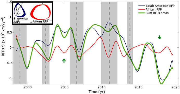
FIGURE 3. Secular acceleration of the areal extent of the RFPs at the CMB. Time evolution of the second derivative of the areal extent of the South American (blue line) and African (red line) RFPs and (green line) the sum of both areal extents at the CMB. The areal extent is calculated as the area within the contour line of −32,000 nT of Br (shown in the map in the figure) using CHAOS-7.2 model until degree 6, monthly from 1998.0 to 2020.2. In dashed vertical gray lines, the mean occurrence times of the well-defined geomagnetic jerks for the last 2 decades are marked. Shaded bands mark the uncertainty of the occurrence times given by one standard deviation. With green arrows other interesting features are indicated (see Discussion in the main text for more details).

We use the CHAOS-7.2 model to estimate the Br of the geomagnetic field, with maximum spherical harmonic degree equal to six in order to avoid the effect of shorter time scales of the higher degrees, which are the most poorly resolved and most affected by model parametrization (see, e.g., Chulliat and Maus, 2014), and be able to isolate both RFPs correctly. By applying the same methodology explained above, we obtain the evolution of $\stackrel{\cdot \cdot }{S}$ of the South American and African RFPs, together and separately, at the CMB as shown in Figure 3. We compare them with the occurrence times of the geomagnetic jerks and see that the minima of $\stackrel{\cdot \cdot }{S}$ of both RFPs together (green curve in Figure 3) are always close to a geomagnetic jerk. In the comparison with the minima of $\stackrel{\cdot \cdot }{S}$ of the SAA at surface (Figure 2C), one could expect that both measures were synchronous or that the minima in Figure 3 (at the CMB) occur before those in Figure 2C (at surface). However, this is not always so. One of the possible explanations of this discrepancy could be related to the fact that not all the minima registered at surface seem to be associated with the same RFP. For instance, the 2013.3 minimum at surface seems to be more likely due to the South American RFP (even if it is interesting to note that it is preceded by a low in the African RFP, which could correlate with 2014 geomagnetic jerk observations from southern African magnetic observatories, Kotzé, 2017). This lack of synchronization between RFPs makes it difficult to provide an accurate estimation of the time occurrence of the minima when both RFPs are considered together, and it reveals the complexity of the mechanisms involved.

According to Terra-Nova et al. (2016), the presence of RFPs at the CMB is due to upwelling of toroidal field from the core, related to temperature anomalies associated with lower mantle lateral heterogeneities (Tarduno et al., 2015; Terra-Nova et al., 2016). In order to interpret our results correctly, we have to take into account that 1) the South American RFP is vanishing while the African RFP is reinforcing (Supplementary Figure S5), 2) the smaller the area of the RFP is, the lower the absolute value of Br minimum in the RFP is (Supplementary Figure S6). This means that in the minima of the second derivative of the areal extent of the RFPs, which seem to be associated with the occurrence of the geomagnetic jerks, there is a decrease in the rate of evolution of the areal extent of the RFPs: the African RFP slows down its extent (slow reinforcement of Br) and the South American RFP vanishes slower (slow weakening of Br). This behavior could be due to a weakening and later reinforcing of the upwelling of toroidal field from the core in the case of the African RFP and vice versa for the South American RFP.

The 2005.0 Minimum and the New Geomagnetic Jerk

In Figures 2C, 3, green arrows have been plotted to highlight two interesting features. The first one is a minimum observed in 2005.1. A geomagnetic jerk in 2005 was already reported by Olsen and Mandea (2008). It had not been well observed in other works (e.g., Brown et al., 2013) but recently some interesting features have been observed around this time (Chulliat and Maus, 2014; Soloviev et al., 2017). Our findings would confirm the existence of an impulse of the geomagnetic field during this epoch. According to previous works (Chulliat et al., 2010; Chulliat and Maus, 2014; Kloss and Finlay, 2019) a geomagnetic jerk is characterized by acceleration changes rapidly before or after a pulse of the secular acceleration (SA) of the geomagnetic field at the CMB. Next, we study the second derivative (i.e., SA) of the Br calculated on regular grid of 10,239 points at the CMB. To be consistent, we apply the same methodology used in the determination of $\stackrel{\cdot \cdot }{S}$ of the SAA and RFPs, but with t_i+1 = t_i + 12 months and t_i−1 = t_i−12 months to provide smoother changes. To estimate the Br of the geomagnetic field, we use the CHAOS-7.2 model with maximum spherical harmonic degree equal to 6 as previously. Then, we calculate the global averaged squared SA of the Br at the CMB monthly during the last 2 decades. We also estimate the global averaged squared SA of Br considering only the positive values (SA of Br+) and negative values (SA of Br−) of the SA of Br in order to evaluate if lobes of some particular sign affect more the occurrence of geomagnetic jerks. Moreover, we also estimate the SA of Br by averaging for a region between 20°S and 70°S in latitude and between 90°W and 70°E in longitude, where the RFPs associated with the SAA at surface are located. The comparison of these estimations with the occurrence of geomagnetic jerks in the last 2 decades (Figure 4) confirms that those occur at the beginning or end of the SA pulses (Chulliat et al., 2010; Chulliat and Maus, 2014). This is also observed when the average is calculated on the region where the RFPs associated with the SAA are located, which reinforces the link between SAA and jerks. In this point, it is worth to mention that observed SA might be a time average of the true instantaneous SA, especially when using geomagnetic field models with temporal damping, such as CHAOS. This could be a limitation to correlate on a very accurate way some features of the SA in time.

FIGURE 4

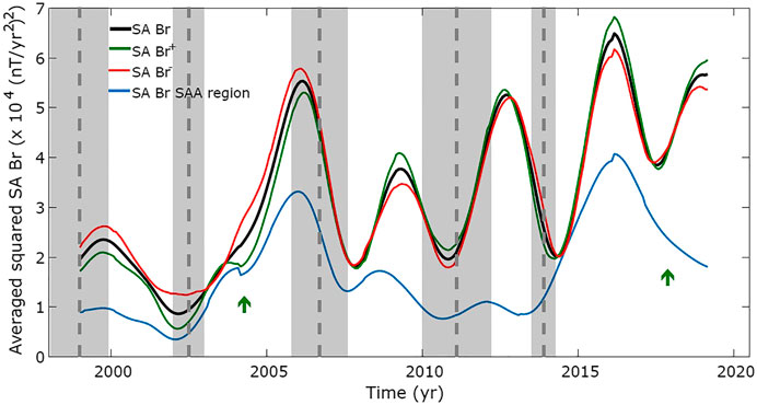
FIGURE 4. Averaged secular acceleration of the geomagnetic field at the CMB. Time variation of the averaged squared secular acceleration of the Br calculated using maximum spherical harmonic degree six at the CMB. In black, the average is calculated globally. In green, we consider only positive lobes of the SA of Br for average. In red, we consider only negative lobes of the SA of Br. In blue, we consider the SA of Br in the region where the RFPs associated with the SAA at surface are located at the CMB (between 20°S and 70°S in latitude and between 90°W and 70°E in longitude). In dashed vertical gray lines, the mean occurrence times of the well-defined geomagnetic jerks for the last 2 decades are marked. Shaded bands mark the uncertainty of the occurrence times given by one standard deviation. With green arrows other interesting features are indicated (see Discussion in the main text for more details).

It seems that there is no clear relation between lobes of a particular sign and the origin of the geomagnetic jerks. However, the asymmetry of the contribution of the negative and positive lobes of SA of Br around 2004.0 is worth noting, registering a slight minimum in the SA of Br+ (also observed when only the region associated with SAA is considered). This means that the contribution of the positive lobes to the SA of the Br decreases in this epoch, which anticipates by some months the minima of acceleration of the areal extent of SAA in 2005.1 (Figure 2C) and of the areal extent of the African RFP (Figure 3). After that, a slight reinforcement of the African RFP is observed around 2006 (black arrow in Supplementary Figure S6).

However, a clear pulse of the SA of the geomagnetic field is not observed around 2005, as would be expected for a geomagnetic jerk. This could mean that the minimum detected in 2005.1 would not correspond with a “typical” geomagnetic jerk (i.e., related to the beginning or end of a pulse of the SA at the CMB). Therefore, this minimum could correspond with a new feature of the geomagnetic field, that is, an impulse related to the asymmetry between positive and negative SA lobes at the CMB. Other possibility is that it is a poor-defined geomagnetic jerk because it is too close to other jerks to clearly identify both with usual tools. Chulliat and Maus (2014) proposed that jerks observed near 2003 and 2005 were related to the same SA pulse, which presents a maximum in 2006. Soloviev et al. (2017) also showed SA pulses around this time. In any case, the analysis of the second derivative of the areal extent of SAA demonstrates to be a promising instrument to identify this kind of poor-defined jerks. Further investigations will be needed in order to confirm these possibilities.

The second interesting feature that is marked with a green arrow in Figures 2C, 3 is the minimum in 2017.8. This corresponds with a new pulse observed in recent times in the SA of Br (Figure 4), with a maximum in 2016.2 and a minimum detected in 2017.5. Both observations could indicate the occurrence of a new geomagnetic jerk as suggested by Brown and Macmillan (2018) and observed by Hammer (2018) and Whaler et al. (2020). Hammer (2018) analyzed the secular variation (SV) and secular acceleration (SA) over ground and virtual observatories calculated from Swarm data and found the characteristic V-shape in the SV and the steep change in the SA in the observatory of Hawaii in the Pacific region in 2017 and in the French Guyana, where the SAA is situated, at the beginning of 2016. Recent studies about the variations in the length of day (LOD) and its relation with the occurrence of geomagnetic jerks support the presence of a geomagnetic jerk in 2017, as well (Duan and Huang, 2020).

Whether the trend of the SAA areal extent does not change, the detection of a relative maximum of $\stackrel{\cdot \cdot }{S}$ of the SAA could indicate coming geomagnetic jerks with around 1.5 years in advance, according to Figure 2C. This is within the mean time of 6–7 years after which no reliable prediction for the field can be made following Qamili et al. (2013).

Finally, a spectral analysis using continuous wavelets applied on the global averaged squared SA of Br and the $\ddot{S}$ of SAA and RFPs series reinforces the found link (Figure 5), by providing a common periodicity of around 2.5–4 years. This not only reinforces the obtained result but also links the SAA with the dynamic of the core associated with the origin of the geomagnetic jerks because the pulses of the SA of Br are related to their occurrence. These results are confirmed by applying the Empirical Mode Decomposition (EMD) following Flandrin (2009) and by estimating the power spectrum in function of the frequency (Supplementary Figure S7 in the Supplementary Material), where a longer period of around 5–10 years is also identified.

FIGURE 5

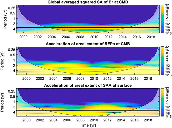
FIGURE 5. Frequency analysis. Wavelet analysis with Morlet basis functions of (upper panel) the global averaged squared secular acceleration of the radial component (Br) of the geomagnetic field at the CMB, (middle panel) second derivative (acceleration) of the areal extent of the South American and African RFPs, and (bottom panel) the second derivative (acceleration) of the areal extent of SAA for the last 2 decades. The shaded plot indicates the nonsignificant part of the analysis and the black lines mark the common period found.

Dynamic Processes at the Core-Mantle Boundary

The relation between geomagnetic jerks and pulses of the global averaged squared SA of the Br at the CMB seems clear from Figure 4 (see also Chulliat et al., 2010; Chulliat and Maus, 2014; Kloss and Finlay, 2019) but also with the SAA (even if with lower amplitudes between 2006 and 2014) as shown by the blue curve of the same figure. This means that possibly the particular core dynamics associated with the SAA, that is, the presence of RFPs at the CMB, is related to the detection of jerks at surface; that is, the SAA area is a region especially sensitive for the identification of geomagnetic jerks.

Chulliat and Maus (2014) carried out a Principal Component Analysis to determine the variability modes (Empirical Orthogonal Functions, EOF) of the SA of the geomagnetic field at the CMB associated with the occurrence of geomagnetic jerks. Three principal modes were obtained: EOF #1 and EOF #2 presented maxima and minima lobes of the SA located in low and middle latitudes of the Atlantic sector (where the SAA is located nowadays); EOF #3 was characterized by maxima and minima of the SA in the Indian sector.

We have estimated the SA of the Br at the CMB during the last 2 decades (see Supplementary Movie S1 in the Supplementary Material) following the methodology mentioned in the previous section. The SA maps of Br corresponding to January 1 for each year are shown in Figure 6. As can be observed, the geomagnetic jerks that occurred in 1999.0 and 2003.0 are dominated by the EOF #3, while the geomagnetic jerks of 2007.0, 2011.0, and 2014.0 are clearly dominated by EOFs #1 and #2. The lowest values of the SA of Br are associated with the 2003.0 geomagnetic jerk. We observe that the lobes over Atlantic sector change their sign after the unfolding of a geomagnetic jerk. Chulliat and Maus (2014) yet noted this feature for 2007.0 and 2011.0 jerks and suggested the presence of a standing magnetohydrodynamic wave with a period of about 6 years at the core surface, described by the sum of the first two EOFs. Torta et al. (2015) also reported on the change of sign in the SA of the geomagnetic field for 2014.0 jerk. More recently, Kloss and Finlay (2019) carried out a detailed analysis of the time-dependent low latitude core flow and geomagnetic field acceleration pulses at the CMB and found an alternated sign of the nonzonal azimuthal flow acceleration at particular longitudinal areas (South Atlantic sector and Indian region). They observed that the rapid acceleration sign changes are related to the occurrence of geomagnetic jerks, focusing their analysis on the 2014 geomagnetic jerk. Here, we note that a new configuration of lobes with opposite sign compared with those observed from 2012.0 to 2014.0 (when the last geomagnetic jerk occurred) is clearly observed in 2016.0 (see also Kloss and Finlay, 2019). This situation (Figures 6R–S) along with the new pulse of SA that was registered in 2016.2 (Figure 4) and the minimum observed in 2017.8 in $\stackrel{\cdot \cdot }{S}$ of the SAA (Figure 2C) and of the RFPs (Figure 3) could indicate the occurrence of a new geomagnetic jerk during these years. In fact, Whaler et al. (2020) found changes in the azimuthal flow acceleration beneath the Pacific region in 2017, which they linked to the occurrence of the geomagnetic jerk that was registered by Hammer (2018) particularly well in observatories in the Pacific. These changes in the flow were accentuated in the west side of the Pacific region, closer to the Indian sector considered as the EOF #3 by Chulliat and Maus (2014). Thus, the new jerk could be dominated by this region, even if it is difficult to identify clearly from Figures 6R–S.

FIGURE 6

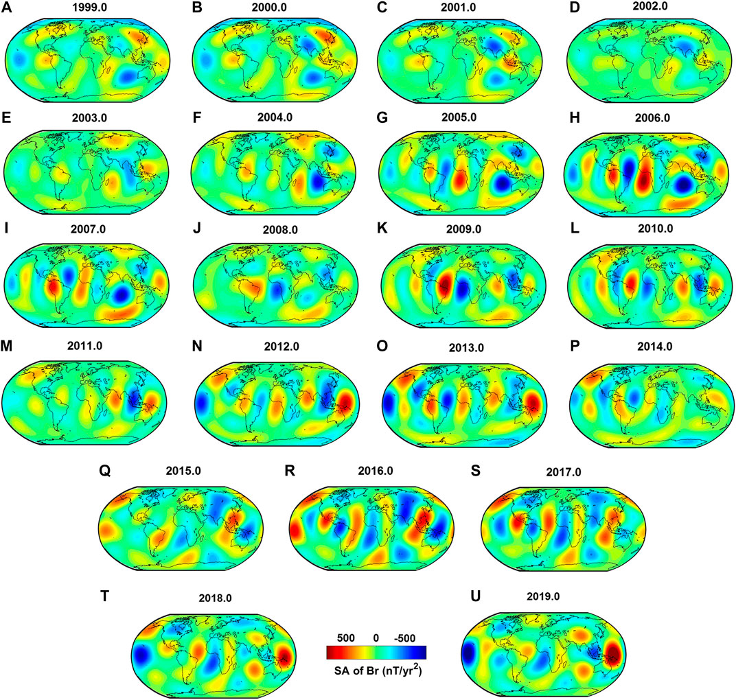
FIGURE 6. Secular acceleration of the Br of the geomagnetic field at the CMB. Maps of the secular acceleration of the Br at CMB for January 1 for every year during the last 2 decades. We use CHAOS-7.2 model until degree six to calculate the Br.

Aubert (2018) proposed that the arrival of quasi-geostrophic Alfvén waves coming from the deep core to the CMB could produce this alternating sign with a period subdecadal. The periods found from the frequency analysis in this work (Figure 5; Supplementary Figure S7) agree with that scenario. Moreover, the flow accelerations are found mainly in the Atlantic and Indian sectors, the same positions where Terra-Nova et al. (2016) observed the presence of RFPs in the last three millennia and the locations of the RFPs associated with the presence of the SAA at surface. The RFPs are related to upwelling of toroidal field from the core, associated with temperature anomalies linked to lower mantle lateral heterogeneities (Tarduno et al., 2015; Terra-Nova et al., 2016). Regarding our work, this could mean that when the upwelling of toroidal field presents a change associated with a minimum in the second derivative of the areal extent of the RFPs and, in turn the SAA, a geomagnetic jerk is observed.

According to Kloss and Finlay (2019), under the Atlantic region a westward motion of azimuthal flow acceleration features is observed. They proposed that it could be due to a quasi-geostrophic Alfvén wavefront that arrives first under western Africa and then moves westwards. This could also agree with part of our results because we observe that the minimum in the second derivative associated with the 2014.0 geomagnetic jerk is observed previously on the areal extent of the African RFP and next on the South American RFP (Figure 3).

The physical mechanism that explains the link between jerks and SAA is not still completely clear, but it seems that the found link between these two apparently different phenomena of the geomagnetic field is an indication that the physical processes that produce the RFPs at the CMB and the SAA at surface involve also the internal dynamics associated with the origin of the geomagnetic jerks. It is possible that the arrival of quasi-geostrophic Alfvén waves at the CMB produces not only nonzonal azimuthal flow accelerations of alternating sign but also effects on the upwelling of toroidal field present at higher latitudes. When a rapid change of the sign of these flow accelerations is produced (Figure 6), this would coincide with a change of the upwelling regime. This could be observed as a pulse of the SA of Br over the RFPs region (Figure 4) and a minimum in the $\stackrel{\cdot \cdot }{S}$ of the RFPs at the CMB (Figure 3) and of the SAA at surface (Figure 2C), and the unfolding of a geomagnetic jerk.

Conclusion

We suggest a previously unreported link between the minima of the second derivative of the areal extent of SAA at surface and the occurrence of geomagnetic jerks for the last 2 decades. This result has been confirmed at the CMB, by studying the areal extent of the RFPs associated with the presence of the SAA at surface.

We have seen that global SA pulses at the CMB related to the occurrence of the geomagnetic jerks are also detected locally on the area at the CMB affected by the RFPs associated with the presence of the SAA at surface.

A new change of sign in the lobes of the SA of Br at the CMB over the Atlantic sector in 2016.0 epoch seems to reinforce the hypothesis proposed by Chulliat and Maus (2014) on the presence of a standing magnetohydrodynamic wave with a 6-year periodicity that is of the order of the periodicities reported in this work. This was also noted by other authors in more recent works (e.g., Aubert, 2018; Kloss and Finlay, 2019). A new pulse has also been observed in the global averaged squared SA of the Br, which has reached a maximum in 2016.2 and a minimum in 2017.5. This fact, along with the change of sign of the lobes of the SA of Br, the analysis of periodicities, and the minima registered in the second derivative of the areal extent of SAA and RFPs in 2017.8, would point to a new geomagnetic jerk. This argument is supported by recent observatory data analyzed by Hammer (2018) where the characteristic V-shape in the secular variation and the steep change in the secular acceleration are found in observatories in the French Guyana in 2016 and Hawaii in 2017.

We have seen that the areal extent of SAA is able to detect through its relative minima all impulses of the geomagnetic field at surface (and, therefore, observed in magnetic observatories). This fact is of particular interest because it could shed light on geomagnetic jerks identified in some, but not all, studies. In this work, the occurrence of the 2005.0 geomagnetic jerk is discussed. We propose that this event, detected as a minimum of the second derivative of the areal extent of SAA, could be an impulse of the geomagnetic field associated with the asymmetry of the positive and negative lobes of the SA of the geomagnetic field at the CMB. It could be considered as a new kind of impulse of the geomagnetic field but also as a poor-defined jerk. It is also important to take into account that the jerks can be poorly defined particularly when we have to distinguish between successive events in disparate regions of the globe that overlap in time. From this point of view, this work is encouraging because it aims to give links to effects at the CMB that help to simplify the view of the surface expressions.

Finally, we have observed that the RFPs at the CMB are mostly observed in the same sectors related to the geomagnetic jerks occurrence (i.e., Atlantic and Indian sectors). The fact of detecting jerks globally (outside of these regions) does not exclude the fact that singular situations of the core dynamics like the presence of RFPs can favor the detection of jerks. These regions seem to be characterized by upwelling of toroidal field from the core, related to temperature anomalies associated with lower mantle lateral heterogeneities (Terra-Nova et al., 2016). Following Kloss and Finlay (2019), it could be possible that the relation between the arrival of quasi-geostrophic Alfvén waves at the CMB and the presence of nonzonal azimuthal flow accelerations of alternating sign could affect the upwelling of toroidal field present in higher latitudes. When a rapid change of the sign of these flow accelerations is produced, this would coincide with a change of the upwelling regime, observed as a minimum in the second derivative of the areal extent of the RFPs at CMB and of the SAA at surface, and the unfolding of a geomagnetic jerk. This could provide an important hint about the dynamic processes that link the RFPs and, therefore, the evolution of the SAA nowadays, with the geomagnetic jerks at the interior of the Earth.

Data Availability Statement

The original contributions presented in the study are included in the article/Supplementary Material, further inquiries can be directed to the corresponding author.

Author Contributions

SAC developed the project and performed the calculations with the help of FJPC. The interpretation of the results and writing were led by SAC with the help of FJPC, ADS, AGL, and EQ; SAC, FJPC, ADS, AGL, and EQ discussed the results and commented on the manuscript.

Funding

The Living Planet Fellowship (TEMPO project) from ESA, Contract No. 4000112784/14/I-Sbo, is the main financial support to this research. ASI Limadou-Science Project has supported this work partially. Grant FPU17/03635 from the Spanish Ministry of Education was funding AGL PhD thesis. FJPC was partially supported by the Spanish research project PGC2018-099103-A-I00.

Conflict of Interest

EQ was employed by the company Serco. The remaining authors declare that the research was conducted in the absence of any commercial or financial relationships that could be construed as a potential conflict of interest.

Acknowledgments

SAC acknowledges The Living Planet Fellowship (TEMPO project) from ESA for providing financial support to this research. SAC and ADS also acknowledge ASI Limadou-Science Project for supporting this work partially. AGL acknowledges the grant FPU17/03635 from the Spanish Ministry of Education. FJPC is grateful to the Spanish research project PGC2018-099103-A-I00. All data and models used to carry out this work can be found in the associated references and in the repository of DTU Space (http://www.space.dtu.dk/english/Research/Scientific_data_and_models/Magnetic_Field_Models). The authors are very grateful to Editor and two reviewers for their useful comments that have helped to improve the quality of this manuscript.

Supplementary Material

The Supplementary Material for this article can be found online at: https://www.frontiersin.org/articles/10.3389/feart.2020.607049/full#supplementary-material.

References

Alexandrescu, M., Gibert, D., Hulot, G., Le Mouël, J.-L., and Saracco, G. (1996). Worldwide wavelet analysis of geomagnetic jerks. J. Geophys. Res. 101, 21975–21994. doi:10.1029/96JB01648

CrossRef Full Text | Google Scholar

Amit, H., Terra-Nova, F., Lézinm, M., and Trindade, R. (2020). Non-monotonous growth and motion of the South Atlantic anomaly. [Preprint]. Available at: https://europepmc.org/article/ppr/ppr156103 (Accessed April 28, 2020).

Google Scholar

Aubert, J. (2018). Geomagnetic acceleration and rapid hydromagnetic wave dynamics in advanced numerical simulations of the geodynamo. Geophys. J. Int. 214, 531–547. doi:10.1093/gji/ggy161

CrossRef Full Text | Google Scholar

Brown, W. J., Mound, J. E., and Livermore, P. W. (2013). Jerks abound: an analysis of geomagnetic observatory data from 1957 to 2008. Phys. Earth Planet. In. 223, 62–76. doi:10.1016/j.pepi.2013.06.001

CrossRef Full Text | Google Scholar

Brown, W. J., and Macmillan, S. (2018). “Geomagnetic jerks during the Swarm era and impact on IGRF-12,” in EGU General Assembly Conference Abstracts, Vienna, Austria, April 8–13, 2018, 20, 7999. Available at: http://nora.nerc.ac.uk/id/eprint/520098 (Accessed May 17, 2018).

Google Scholar

Campuzano, S. A., Gómez-Paccard, M., Pavón-Carrasco, F. J., and Osete, M. L. (2019). Emergence and evolution of the south Atlantic anomaly revealed by the new paleomagnetic reconstruction SHAWQ2k. Earth Planet. Sci. Lett. 512, 17–26. doi:10.1016/j.epsl.2019.01.050

CrossRef Full Text | Google Scholar

Chulliat, A., Thébault, E., and Hulot, G. (2010). Core field acceleration pulse as a common cause of the 2003 and 2007 geomagnetic jerks. Geophys. Res. Lett. 37, L07301. doi:10.1029/2009GL042019

CrossRef Full Text | Google Scholar

Chulliat, A., and Maus, S. (2014). Geomagnetic secular acceleration, jerks, and a localized standing wave at the core surface from 2000 to 2010. J. Geophys. Res. Solid Earth. 119, 1531–1543. doi:10.1002/2013JB010604

CrossRef Full Text | Google Scholar

Courtillot, V., Ducruix, L., and Le Mouel, J. L. (1978). Sur une accélération récente de la variation séculaire du champ magnétique terrestre. C. R. Acad. Sci. Paris. 287, 1095–1098. https://www.ipgp.fr/fr/une-acceleration-recente-de-variation-seculaire-champ-magnetique-terrestre

Google Scholar

De Santis, A., Qamili, E., Spada, G., and Gasperini, P. (2012). Geomagnetic South Atlantic Anomaly and global sea level rise: a direct connection? J. Atmos. Sol. Terr. Phys. 74, 129–135. doi:10.1016/j.jastp.2011.10.015

CrossRef Full Text | Google Scholar

De Santis, A., Qamili, E., and Wu, L. X. (2013). Toward a possible next geomagnetic transition? Nat. Hazards Earth Syst. Sci. 13, 3395–3403. doi:10.5194/nhess-13-3395-2013

CrossRef Full Text | Google Scholar

Domingos, J., Jault, D., Pais, M. A., and Mandea, M. (2017). The South Atlantic anomaly throughout the solar cycle, Earth Planet Sci. Lett. 473, 154–163. doi:10.1016/j.epsl.2017.06.004

CrossRef Full Text | Google Scholar

Duan, P., and Huang, C. (2020). Intradecadal variations in length of day and their correspondence with geomagnetic jerks. Nat. Commun. 11, 2273. doi:10.1038/s41467-020-16109-8

PubMed Abstract | CrossRef Full Text | Google Scholar

Finlay, C. C., Aubert, J., and Gillet, N. (2016a). Gyre-driven decay of the Earth’s magnetic dipole. Nat. Commun. 7, 10422. doi:10.1038/ncomms10422

PubMed Abstract | CrossRef Full Text | Google Scholar

Finlay, C. C., Kloss, C., Olsen, N., Hammer, M., Toeffner-Clausen, L., Grayver, A., et al. (2020). The CHAOS-7 geomagnetic field model and observed changes in the South Atlantic Anomaly. Earth Planets Space. 72. doi:10.1186/s40623-020-01252-9

Google Scholar

Finlay, C. C., Olsen, N., Kotsiaros, S., Gillet, N., and Tøffner-Clausen, L. (2016b). Recent geomagnetic secular variation from Swarm and ground observatories as estimated in the CHAOS-6 geomagnetic field model. Earth Planets Space. 68, 112. doi:10.1186/s40623-016-0486-1

CrossRef Full Text | Google Scholar

Flandrin, P. (2009). Matlab toolbox: empirical mode decomposition. Available at: http://perso.ens-lyon.fr/patrick.flandrin/software2.html (Accessed February 26, 2009).

Google Scholar

Friis-Christensen, E., Lühr, H., and Hulot, G. (2006). Swarm: a constellation to study the Earth’s magnetic field. Earth Planets Space. 58, 351–358. doi:10.1186/bf03351933

CrossRef Full Text | Google Scholar

Gillet, N. (2019). “Spatial and temporal changes of the geomagnetic field: insights from forward and inverse core field models,” in Geomagnetism, aeronomy and space weather: a journey from the Earth's core to the sun. Editors M. Mandea, M. Korte, A. Yau, and E. Petrovsky (Cambridge, England: Cambridge University Press), 115–132.

CrossRef Full Text | Google Scholar

Gubbins, D., Jones, A. L., and Finlay, C. C. (2006). Fall in Earth's magnetic field is erratic, in Science. 312 (5775), 900–902. doi:10.1126/science.1124855

CrossRef Full Text | Google Scholar

Hammer, M. D. (2018). Local estimation of the Earth’s core magnetic field. PhD thesis. Kongens Lyngby (Denmark): Technical University of Denmark (DTU).

Google Scholar

Hulot, G., Eymin, C., Langlais, B., Mandea, M., and Olsen, N. (2002). Small scale structure of the geodynamo inferred from Oersted and Magsat satellite data. Nature. 416, 620–623. doi:10.1038/416620a

PubMed Abstract | CrossRef Full Text | Google Scholar

Jackson, A., Jonkers, A. R. T., and Walker, M. R. (2000). Four centuries of geomagnetic secular variation from historical records, Philos. Trans. Roy. Soc. London Ser. A. 358 (1768), 957–990. doi:10.1098/rsta.2000.0569

CrossRef Full Text | Google Scholar

Kim, H. R., and von Frese, R. R. B. (2013). Localized analysis of polar geomagnetic jerks. Tectonophysics. 585, 26–33. doi:10.1016/j.tecto.2012.06.038

CrossRef Full Text | Google Scholar

Kloss, C., and Finlay, C. C. (2019). Time-dependent low-latitude core flow and geomagnetic field acceleration pulses. Geophys. J. Int. 217 (1), 140–168. doi:10.1093/gji/ggy545

CrossRef Full Text | Google Scholar

Kotzé, P. B. (2017). The 2014 geomagnetic jerk as observed by southern African magnetic observatories. Earth Planets Space. 69, 17. doi:10.1186/s40623-017-0605-7

CrossRef Full Text | Google Scholar

Laj, C., and Kissel, C. (2015). An impending geomagnetic transition? Hints from the past. Front. Earth Sci. 3, 10. doi:10.3389/feart.2015.00061

CrossRef Full Text | Google Scholar

Lesur, V., Wardinski, I., Hamoudi, M., Rother, M., and Kunagu, P. (2011). “Third version of the GFZ reference internal magnetic model: GRIMM-3, IUGG2011, MR207,” in 25th IUGG General Assembly, Melbourne, Australia, June 27–July 8, 2011, 1356 (4), 1345–1378. Available at: https://gfzpublic.gfz-potsdam.de/pubman/item/item_243756 (Accessed July 7, 2011).

Google Scholar

Lesur, V., Wardinski, I., Hamoudi, M., and Rother, M. (2010). The second generation of the GFZ reference internal magnetic model: GRIMM-2. Earth Planets Space. 62 (6), 765–773. doi:10.5047/eps.2010.07.007

CrossRef Full Text | Google Scholar

Malin, S. R. C., Hodder, B. M., and Barraclough, D. R. (1983). “Geomagnetic secular variation: a jerk in 1970,” in Publicaciones del Observatorio del Ebro. Memoria. Roquetes, Spain: Observatori de l’Ebre, Vol. 14, 239–256.

Google Scholar

Mandea, M., Holme, R., Pais, A., Pinheiro, K., Jackson, A., and Verbanac, G. (2010). Geomagnetic jerks: rapid core field variations and core dynamics. Space Sci. Rev. 155, 147–175. doi:10.1007/s11214-010-9663-x

CrossRef Full Text | Google Scholar

Mandea, M., and Macmillan, S. (2000). International geomagnetic reference field—the eighth generation. Earth Planets Space. 52, 1119–1124. doi:10.1186/bf03352342

CrossRef Full Text | Google Scholar

Olsen, N., and Haagmans, R. (2006). Swarm—the Earth’s magnetic field and environment explorers. special issue. Earth Planets Space. 58, 349–496. doi:10.1186/bf03351932

CrossRef Full Text | Google Scholar

Olsen, N., and Mandea, M. (2008). Rapidly changing flows in the Earth’s core. Nat. Geosci. 1 (6), 390–394. doi:10.1038/ngeo203

CrossRef Full Text | Google Scholar

Olsen, N., Mandea, M., Sabaka, T. J., and Tøffner-Clausen, L. (2009). CHAOS-2–A geomagnetic field model derived from one decade of continuous satellite data. Geophys. J. Int. 179, 1477–1487. doi:10.1111/j.1365-246X.2009.04386.x

CrossRef Full Text | Google Scholar

Olson, P., and Amit, H. (2006). Changes in Earth’s dipole. Naturwissenschaften. 93, 519–542. doi:10.1007/s00114-006-0138-6

PubMed Abstract | CrossRef Full Text | Google Scholar

Pavón-Carrasco, F. J., and De Santis, A. (2016). The South Atlantic anomaly: the key for a possible geomagnetic reversal. Front. Earth Sci. 4, 40. doi:10.3389/feart.2016.00040

CrossRef Full Text | Google Scholar

Pinheiro, K. J., Jackson, A., and Finlay, C. C. (2011). Measurements and uncertainties of the occurrence time of the 1969, 1978, 1991, and 1999 geomagnetic jerks. Geochem. Geophys. Geosyst. 12, Q10015. doi:10.1029/2011GC003706

CrossRef Full Text | Google Scholar

Qamili, E., De Santis, A., Isac, A., Mandea, M., Duka, B., and Simonyan, A. (2013). Geomagnetic jerks as chaotic fluctuations of the Earth’s magnetic field. Geochem. Geophys. Geosyst. 14, 839–850. doi:10.1029/2012GC004398

CrossRef Full Text | Google Scholar

Soloviev, A., Chulliat, A., and Bogoutdinov, S. (2017). Detection of secular acceleration pulses from magnetic observatory data. Phys. Earth Planet. In. 270, 128–142. doi:10.1016/j.pepi.2017.07.005

CrossRef Full Text | Google Scholar

Tarduno, J. A., Watkeys, M. K., Huffman, T. N., Cottrell, R. D., Blackman, E. G., Wendt, A., et al. (2015). Antiquity of the South Atlantic Anomaly and evidence for top-down control on the geodynamo. Nat. Commun. 6, doi:10.1038/ncomms8865

CrossRef Full Text | Google Scholar

Terra-Nova, F., Amit, H., Hartmann, G. A., Trindade, R. I. F., and Pinheiro, K. J. (2017). Relating the South Atlantic anomaly and geomagnetic flux patches. Phys. Earth Planet. In. 266, 39–53. doi:10.1016/j.pepi.2017.03.002

CrossRef Full Text | Google Scholar

Terra-Nova, F., Amit, H., Hartmann, G. A., and Trindade, R. I. F. (2015). The time dependence of reversed archeomagnetic flux patches. J. Geophys. Res. Solid Earth. 120, 691–704. doi:10.1002/2014JB011742

CrossRef Full Text | Google Scholar

Terra-Nova, F., Amit, H., Hartmann, G. A., and Trindade, R. I. F. (2016). Using archaeomagnetic field models to constrain the physics of the core: robustness and preferred locations of reversed flux patches. Geophys. J. Int. 206 (3), 1890–1913. doi:10.1093/gji/ggw248

CrossRef Full Text | Google Scholar

Torta, J. M., Pavón‐Carrasco, F. J., Marsal, S., and Finlay, C. C. (2015). Evidence for a new geomagnetic jerk in 2014. Geophys. Res. Lett. 42, 7933–7940. doi:10.1002/2015GL065501

CrossRef Full Text | Google Scholar

Tozzi, R., De Michelis, P., and Meloni, A. (2009). Geomagnetic jerks in the polar regions. Geophys. Res. Lett. 36, L15304. doi:10.1029/2009GL039359

CrossRef Full Text | Google Scholar

Whaler, K., Hammer, M., Finlay, C., and Olsen, N. (2020). “Core-mantle boundary flows obtained purely from Swarm secular variation gradient information,” in 22nd EGU General Assembly, Vienna, Austria, May 4–8, 2020. Available at: https://doi.org/10.5194/egusphere-egu2020-9616 (Accessed April 30, 2020).

Google Scholar