Near-Field Body-Wave Extraction From Ambient Seafloor Noise in the Nankai Subduction Zone

Introduction

Ambient noise analysis applied to land-based seismic records has retrieved various wavefields propagating between two receivers (Wapenaar, 2004). Retrieved waves are mainly surface waves (e.g., Sabra, 2005; Shapiro et al., 2005), but body wave retrievals by correlating ambient noises from land-based observations have also been reported (Roux et al., 2005; Draganov et al., 2007; Zhan et al., 2010; Poli et al., 2011; Ryberg, 2011; Takagi et al., 2014). In particular, reflections from the 410 and 660 km discontinuities in the upper mantle could be detected from ambient noise records observed in Finland (Poli et al., 2012). Body waves propagating through the deep interior of the Earth, including core phases, have been extracted using globally distributed broadband seismometers (Nishida, 2013). Near the coastline, direct and refracted P waves could be detected by a dense array of seismometers deployed at Long Beach, California, and those waves can be used to estimate the three-dimensional (3D) velocity structure at shallow depth (Nakata et al., 2015).

The difficulty of extracting body waves is primarily caused by large amplitudes of surface waves observed at land stations, which correspond to microseisms excited by ocean swells in the ocean areas (Longuet-Higgins, 1950; Hasselmann, 1963). Retrievals of body waves may be owing to either large amplitudes of body waves excited by ocean swells near the coastline (Nakata et al., 2015) or low amplitude of surface waves in quiet regions that are away from the coastlines. On the other hand, for seafloor observations, if wave-wave interactions of ocean swell persistently excites microseisms including body and surface waves, seafloor sensors may capture such signals because they are close to excitation regions of the microseisms. Waves extracted from seafloor observations are primarily surface waves, including Rayleigh waves, Love waves, their higher modes (e.g., Takeo et al., 2013; Lin et al., 2016; Isse et al., 2019; Kawano et al., 2020), Scholte waves (Mordret et al., 2014), and ocean acoustically-coupled Rayleigh (ACR) waves (Ewing et al., 1957; Sugioka et al., 2001; Butler and Lomnitz, 2002; Butler, 2006). Here, ACR waves (or seismoacoustic modes) can be observed at frequencies of 0.5–5.0 Hz, which include higher modes of Rayleigh waves whose energies are distributed in the ocean and marine sediment, and have a propagation velocity slightly less than 1.5 km/s (Tonegawa et al., 2015). However, teleseismic body waves excited in the ocean areas can be observed at land stations (Gerstoft et al., 2006; Koper et al., 2010; Landès et al., 2010; Gualtieri et al., 2014; Farra et al., 2016; Nishida and Takagi, 2016). Although this means that most of the body wave energy is transmitted to the interior of the Earth and can be observed at distant stations, near-field body waves are also possibly observed under the conditions of dense seismic sensors deployed at the seafloor.

In the Nankai subduction zone, south of Japan, the Philippine Sea Plate (PHS) subducts northwestwards from the Nankai Trough, historically leading to megathrust earthquakes along the plate boundary. To investigate the seismic structure of the subduction zone, seismic exploration surveys have been conducted with dense survey lines, in which temporary ocean bottom seismometers (OBSs), each equipped with a hydrophone, have been deployed for refraction surveys (e.g., Nakanishi et al., 2018). Moreover, to monitor seismic activity in this region, a permanent cabled-network of seismometers and pressure gauges (Dense Oceanfloor Network System for Earthquakes and Tsunamis: DONET) (Kaneda et al., 2015; Kawaguchi et al., 2015) has been installed on the accretionary prism where the bathymetry from the trough gradually becomes shallower landwards to a distance of 30–40 km, after which it is almost flat until 20–30 km before the coastline.

To explore the retrieval of body waves propagating between two seafloor receivers, we employed ambient noise records acquired by seismometers and pressure sensors of DONET and temporary OBSs. Such retrievals have potential for investigating the 3D seismic structure beneath the seafloor without natural and artificial seismic sources. In this study, we show near-field P-wave extractions at frequencies of 0.2–0.5 Hz from seafloor pressure gauges, mainly deployed at the slope bathymetry region, and those at frequencies of 1–3 Hz from seafloor seismometers, mainly deployed at the flat bathymetry region. Those extractions are further examined by 2D numerical simulations.

Materials and Methods

Station Data

The continuous records used in this study consist of three-component seafloor motions and pressure fluctuation and were acquired by broadband seismometers and differential pressure gauges (DPGs) at each station of DONET and 4.5 Hz short-period sensors and hydrophones at each temporary station. The broadband seismometers (Guralp CMG-3T) of DONET were buried 1 m below the seafloor, and have a flat velocity response from 100 Hz to 360 s (e.g., Nakano et al., 2013). The response of the hydrophone decreases from 2 Hz to lower frequencies (e.g., Tonegawa et al., 2015). Also used were the three components of a broadband seismometer deployed in a borehole at a depth of 900 m from the seafloor (Kopf et al., 2011; 2016), at which lower noise levels than those at the seafloor are observed due to the amplitude decay of persistently propagating surface waves. The sampling rates of all sensors are decimated to 40 Hz. The stations in DONET are installed in the eastern (DONET1) and western (DONET2) part of the Nankai subduction zone with a station spacing of 15–20 km, whereas the temporary stations are distributed along five lines that cover the central to eastern part of the subduction zone with a station spacing of 5 km (Figure 1). The observation periods of DONET and temporary stations are 2011∼present and September–December of 2011, respectively. We prepared two datasets of the continuous records to retrieve wavefields of lower (0.2–0.5 Hz) and higher frequency (1–3 Hz) components using an ambient noise analysis. Dataset 1 for the lower frequency range includes all four components of 49 stations of DONET and the three components of the borehole sensor, connected to the DONET cable, for February–March of 2016 (Figure 1). Dataset 2 for the higher frequency range includes all four components of 20 DONET stations and 150 temporary stations for October–November of 2011 (Figure 1). Moreover, an additional dataset was prepared covering the middle frequency range (0.5–1.0 Hz) from DONET records for February–March of 2016. We did not use records of DONET2 in Dataset 2 because it had not yet been installed in 2011.

FIGURE 1

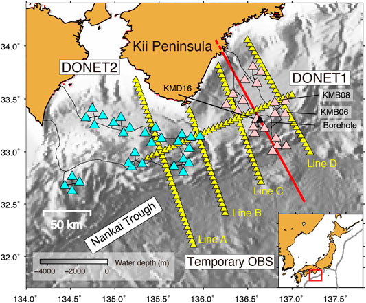
FIGURE 1. Map showing the stations used in this study. Yellow, pink, and light-blue triangles represent temporary, DONET1, and DONET2 stations, respectively. The black triangle indicates the borehole location. The red line show the location of Vp structure (Nakanishi et al., 2008) used in the numerical simulation. The dashed red line represents the region where the one-dimensional profile at the northern edge of the Vp structure is extended.

Cross-Correlation Function Calculation

Cross-correlation functions (CCFs) were calculated with ambient noise records in which energetic signals including earthquakes were suppressed by the following log-normal shaped function.

$F\left(t\right)=\frac{1}{\sqrt{2\pi \sigma \left(t/T\right)}}\text{exp}\left\{-\frac{{\left(\log \left(\frac{t}{T}\right)\right)}^2}{2{\sigma }^2}\right\}(1)$

where σ = 2 and the time length, T = 400 s. When σ > 1 in Equation 1, the peak of the function is located forward and its tail amplitude is still preserved at the end of the time length (Supplementary Figure S1). The time length, T, was determined from the durations of relatively large earthquake signals at 0.2–0.5 Hz observed by DONET. Supplementary Figure S1A shows a waveform example for a deep earthquake with a magnitude of 5.7, a depth of 410 km (earthquake catalog from United States Geological Survey), and an epicentral distance of 3.67°. The coda amplitudes can be observed for a duration of ∼400 s. If the coda portions of earthquakes are longer than 400 s and still have large amplitudes (see Equations 2, 3 for amplitude criteria), Equation 1 is repetitively applied to the rest of the coda. A cosine taper with a time window of 20 s was also applied to both the edges of the function. The root-mean-squared (RMS_1hour) amplitudes were calculated with 1-h continuous records at a frequency of 0.2–0.5 Hz. When amplitudes in the 1-h record at 0.2–0.5 Hz, A_max, exceed five times the RMS_1hour, the raw records were divided by the following function with a time shift of 80 s from the time of A_max:

$S\left(t\right)=C\cdot F\left(t\right)(2)$

where

$C=3A_{max}/RM{S}_{1hour}(3)$

The reason of the time shift is that the maximum amplitude of the log-normal shaped function (Equation 1) is approximately 80 s from the starting time. In addition, when moderate-sized earthquakes occur in Japan, the large and small amplitudes of the S and P waves within an S–P time of <80 s are observed, and the S wave amplitude often corresponds to A_max. Equation 2 with a time shift of 80 s and Equation 3 can effectively suppress the large amplitudes of such earthquake signals. An example of the suppression of the deep earthquake signals is shown in Supplementary Figure S1D. The CCFs were calculated using a time window of 200 s with spectral whitening (Brenguier et al., 2007). The CCFs were stacked over 2 months. When the RMS of one segment (200 s) in the processed records was less than 0.3 times the RMS_1hour, the CCFs of those segments were discarded.

Previous studies calculated CCFs using continuous records with one-bit normalization where amplitudes are equalized while preserving their polarities. Using the continuous records acquired by a borehole sensor and a nearby seafloor sensor (KMD16, Figure 1) with a horizontal separation distance of 3.7 km, we compared the resulting CCFs (Figure 2). Without one-bit normalization they show P waves and ACR waves at lag times of ±2 s and +4 s, respectively, while with one-bit normalization the CCFs do not show any clear signals. The reasons for the absence of clear signals remains elusive, but we suppose that larger and smaller amplitudes in the ambient seafloor noise are dominated by different wavefields, as will be discussed in Discussion. In this study, we preserved amplitude information in the continuous records with suppressing energetic signals when calculating CCFs. Because CCFs calculated with spectral whitening measure the phase difference between two time series (e.g., Prieto et al., 2009; Tonegawa et al., 2009), the phase difference obtained in the CCFs reflects portions of the time series with relatively large amplitudes.

FIGURE 2

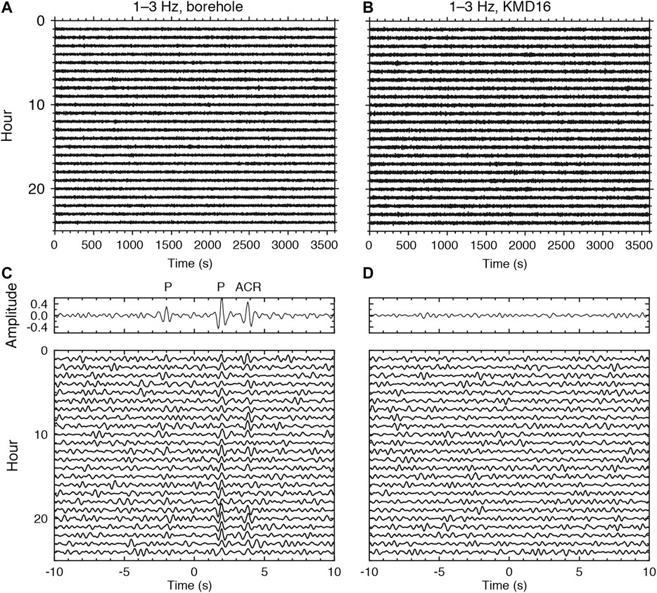
FIGURE 2. Waveform examples recorded with borehole and seafloor sensors. (A) One-hour records of the vertical component at 1–3 Hz observed at the borehole sensor on February 9, 2016. (B) Same as (A), but for KMD16. (C) One-hour CCFs using the waveforms in (A,B), with the borehole as the reference site. The top panel represents the CCF stacked over the CCFs in the bottom panel. (D) Same as (C), but for applying a one-bit normalization to the waveforms in (A,B).

Results

Supplementary Figure S2 shows CCFs for 4 × 4 components at 0.2–0.5 Hz. Most of the component combinations only show ACR wave propagations with a propagation velocity of 1.5 km s⁻¹ or surface waves with slower velocities, whereas pressure-pressure (P-P) CCFs show body wave propagations. In Figure 3, the reference station is located at a lower latitude, so that signals in the positive lag time represent waves propagating northwards. P wave propagations are observed up to a separation distance of 17 km in the positive lag time along the travel time curve of the P waves estimated from the velocity structure (Tonegawa et al., 2017). Here, we constructed a one-dimensional (1D) velocity model averaged over all of the 1D velocity profiles obtained from the DONET stations below the seafloor (Tonegawa et al., 2017). The P wave can be observed in the positive lag time of the CCF for the station pair of KMB06 and KMB08 (Figure 3D). The turning depth of P waves reaches up to 6 km from the seafloor (Figure 3), which samples the plate boundary in the shallow subduction zone.

FIGURE 3

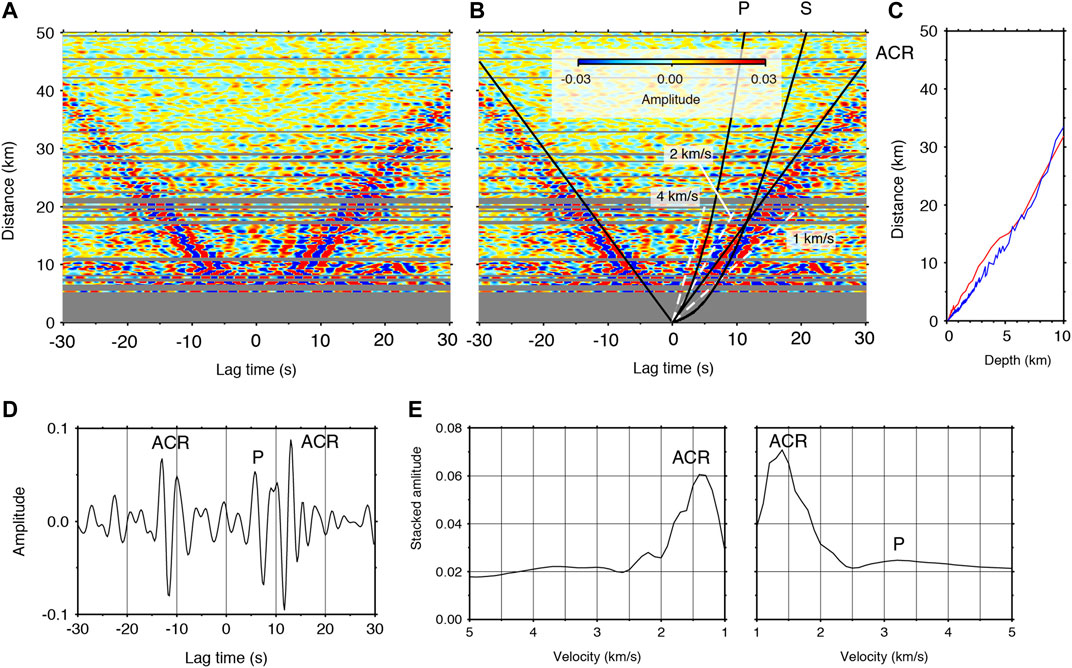
FIGURE 3. CCFs aligned as a function of the separation distance of two stations. (A) P-P CCFs at 0.2–0.5 Hz using DPG records. (B) Same as (A), but with travel time curves of P and S waves calculated with a velocity model (Tonegawa et al., 2017), and a solid line with a propagation velocity of 1.5 km/s. White dashed lines represent apparent velocities of 1, 2, and 4 km/s. (C) The bottoming depth of (red) P and (blue) S waves calculated using the velocity model (Tonegawa et al., 2017). (D) A stacked P-P CCF at 0.2–0.5 Hz for the KMB06–KMB08 station pair, with a separation distance of 14.0 km. (E) Slant stack results for (left) negative and (right) positive lag times of the CCFs in (A).

Figure 4 shows P-P and vertical-vertical (Z-Z) CCFs at 1.0–3.0 Hz. Although P waves were observed in the P-P CCFs at 0.2–0.5 Hz, in the P-P CCFs at 1.0–3.0 Hz only ACR waves were observed. Instead, P waves were retrieved in the positive and negative lag times of the Z-Z CCFs at 1.0–3.0 Hz, and they reach up to 11 km in separation distance of two stations. At the middle frequency range of 0.5–1.0 Hz, we did not extract body waves (Supplementary Figure S3), and hence focus on body wave retrieval at the frequency bands of 0.2–0.5 Hz and 1.0–3.0 Hz in the subsequent sections.

FIGURE 4

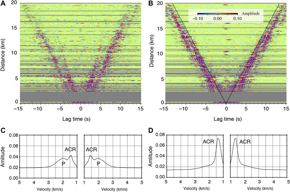
FIGURE 4. CCFs aligned as a function of the separation distance of two stations. (A) Z-Z CCFs at 1–3 Hz using short-period sensor. (B) Same as (A), but for P-P CCFs using hydrophone. Solid line indicates a wave propagation with a velocity of 1.5 km/s. (C) Slant stack results for (left) negative and (right) positive lag times of the CCFs in (A). (D) Same as (C), but for the CCFs in (B).

To confirm the stability of the obtained CCFs, we compared them for stacking periods of 3 months, 1 month, and 2 weeks in the low frequency band (Supplementary Figure S4). Because the observation period of Dataset 2 was almost 2 months, we did not confirm the stability of Dataset 2. The CCFs were almost stable over all of the stacking periods; hence, we discuss the characteristics of the retrieved waves based on a 2 months stacking period.

Discussion

P Wave Retrieval

We measured the apparent velocities of P waves in high and low frequency bands using a slant stack technique. Given apparent velocities, the theoretical travel times can be calculated using the distances between two stations. The apparent velocity was varied between 1 km/s and 5 km/s, with an increment of 0.1 km/s. We averaged the absolute amplitudes of the CCFs within a 0.5 s time window from the theoretical travel time. The averaged values were stacked for the separation distances between two stations: less than 10 and 17 km for the high and low frequency bands, respectively, because large amplitudes were obtained in the distance ranges (Figures 3, 4). This process was performed for positive and negative lag times.

We obtained velocities of 2.0 km/s in the high frequency band (Figure 4) and 3.2 km/s for positive lag times in the low frequency band (Figure 3). This velocity difference and the fact that P waves in the low frequency band propagate over relatively long distances indicate that the turning depths of these P waves were relatively shallow and deep, respectively, and the apparent velocities reflect the P-wave velocity structure (Vp) at these depths. Indeed, the travel time curve gradient of the P waves gradually increased as a function of distance (Figure 3B), which reflects the vertical velocity gradient of the accretionary prism. Seismic exploration surveys of the entire Nankai accretionary prism have also reported a Vp of 2.0–4.0 km/s in the marine sediments and a gradual increases with depth of the Vp structure at shallower depths in the accretionary prism (e.g., Kodaira et al., 2002; Takahashi et al., 2002; Nakanishi et al., 2008). In the higher frequency band, because the turning depth is relatively shallow, the turning P waves are simply observed at stations with separation distances less than 11 km. For the low frequency band, because the turning depth is close to the plate boundary, if seismic velocity discontinuities are present near the bottom of the prism, refracted and head waves can be generated. Indeed, the presence of a low velocity layer has been reported at the bottom of the accretionary prism in the southern DONET1 region (Park et al., 2010; Kamei et al., 2012; Akuhara et al., 2020). In this study, for the low frequency observations from DONET1, the retrieved P waves may contain such multiple P phases.

In order to investigate the region where P waves were retrieved at 0.2–0.5 Hz, we selected P-P CCFs that contain P waves by cross-correlating between the reference CCF and individual P-P CCFs, which is a similar approach to that of a previous study (Nakata et al., 2015). The reference CCF was calculated by stacking the P-P CCFs of all station pairs within separation distances of 10–17 km along the travel time curve of the P waves shown in Figure 3B (Tonegawa et al., 2017). We calculated the cross-correlation coefficients (CC) between the reference CCF and individual P-P CCFs with a time window of ±2 s from the travel time curve. If CC > 0.6, we consider that the CCF possibly contains P waves, and plot the pair in the map (red lines in Figure 5A). As a result, pairs showing P waves are primarily concentrated at the southern part of DONET, where the seafloor slope to the trough is formed.

FIGURE 5

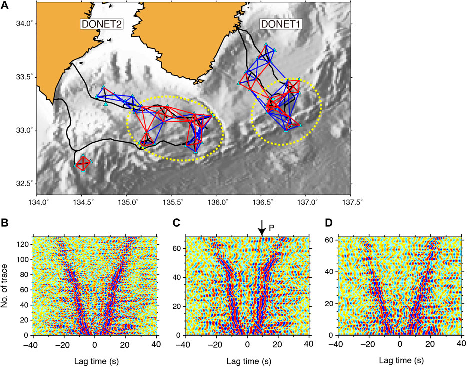
FIGURE 5. Screening of CCFs that show P wave extractions. (A) Map showing pairs that (red line) shows P wave extractions and those that (blue line) do not show P extractions. Dotted yellow ellipses represent the regions where P waves are extracted. (B) P-P CCFs at 0.2–0.5 Hz ordered by separation distance of two stations (C) P-P CCFs that contain P waves are selected from CCFs in (B). (D) P-P CCFs that do not contain P waves are selected from CCFs in (B).

To explore the regions where P waves are observed at 1.0–3.0 Hz, we aligned Z-Z CCFs with the separation distance of two stations of 5 km along Lines A-D (Figure 1). Because the separation distances in the temporary OBS array were equal, aligning the CCFs with 5 km separation distances along lines allowed us to compare the retrieved waves with the geological setting. The result shows that P waves were primarily retrieved at the flat bathymetry region, while signals were weak at the slope bathymetry region (Figure 6). This contrasts with the retrieval of P wave at 0.2–0.5 Hz. Note that the retrieved P waves in the Z-Z CCFs are different from the ACR waves detected in the P-P CCFs using hydrophone records in a previous study (Supplementary Figure S5) (Tonegawa et al., 2015), in which the P waves in the Z-Z CCFs were faster.

FIGURE 6

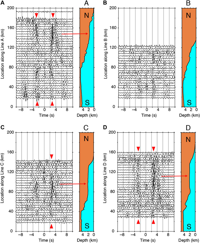
FIGURE 6. P wave retrieval at 1–3 Hz. (A) Z-Z CCFs for pairs whose separation distance is 5 km are aligned along line A (Figure 1). Red triangles represent P wave retrievals, and red arrow indicates the location where the P wave is retrieved, which corresponds to the flat bathymetry region. Right panel shows the bathymetry along the line A. (B) Same as (A), but for line B. (C) Same as (A), but for line C. (D) Same as (A), but for line D.

Previous studies that retrieved body waves at land stations speculated that body waves are converted from the Rayleigh waves due to the heterogeneous structure of the Earth’s upper crust (Roux et al., 2005), and that there are specific structures where body wave energy is trapped and scattered, such as low velocity layers, basins, topography, and heterogeneity (Zhan et al., 2010). Although the retrieved P waves retrieved in our observations may have included contributions from the correlation of P waves trapped and scattered by heterogeneities within the accretionary prism toe, in which the original P waves were generated by wave-wave interactions at the sea surface, the wavelength of the P wave at low frequency was 15 km, for a frequency of 0.2 Hz and a propagation velocity of 3.0 km/s. This wavelength appears to be long for sufficient seismic wave scattering. Therefore, we conducted numerical simulations to evaluate the contribution of the original P waves associated with wave-wave interactions to the P waves extracted from our observations.

Wave Propagation From Numerical Simulation

In this section, we confirm whether the characteristics of the waves retrieved from ambient seafloor noises can be reproduced by a simple 2D numerical simulation for the ocean-solid Earth system. Since it appears that P retrieval is related to the slope and flat regions in the bathymetry, we compare wave propagations depending on frequency (0.2–0.5 Hz and 1–3 Hz), source locations (slope and flat), and component (vertical velocity and stress τ_zz). We used a 2D finite difference method with a rotated-staggered grid for second order approximations in time and space (Saenger et al., 2000). The calculation has been performed in the displacement-stress scheme with an absorbing boundary condition (Clayton and Engquist, 1977), and converted the vertical displacement to vertical velocity seismograms to compare with the τ_zz component. We applied vertical single forces with Ricker wavelets for central (maximum) frequencies of 2.0 Hz (2.9 Hz) and 0.35 Hz (0.5 Hz), respectively, to produce wavefields at high and low frequencies. The grid size is 10 × 10 m and 20 × 20 m for high and low frequencies, respectively. Stations are set at the seafloor within a distance ranging between 0 and 200 km with an interval of 1 km.

The seismic velocity structure at the subseafloor is based on a Vp structure resulting from a seismic exploration survey (Figures 1, 7A) (Nakanishi et al., 2008). The 1D Vp profile at the northern edge of the model is extended landward (Figure 1). The Vs and density were derived from Vp using empirical relations (Brocher, 2005). A 1D profile (depth dependent) of the Vp is applied to the sea water (Munk, 1974), while Vs and density are 0 and 1.02 g/cm³, respectively. The calculation was unstable in the cases where Vp/Vs of the accretionary prism at shallow depths was large and the small horizontal-scale bathymetry was complex. To avoid these problems, we set Vp/Vs = 2.5 when Vp/Vs > 2.5 and applied a horizontal distance moving average of 10 km to the seafloor. The minimum Vs is 0.56 km/s because the minimum Vp in the sea water is approximately 1.4 km/s (Munk, 1974). The source locations were set to horizontal distances of 80 and 110 km at the sea surface, which correspond to the slope and flat bathymetry regions, respectively (Figure 7A).

FIGURE 7

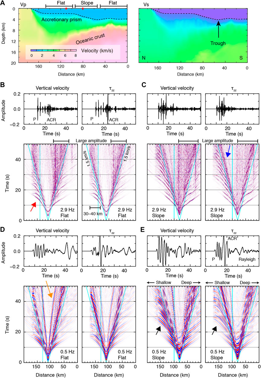
FIGURE 7. Two-dimensional numerical simulation for wave propagation. (A)Vp model used in the numerical simulation. The dotted line shows the bathymetry. Red stars at 80 and 110 km in horizontal distance show the source locations at the sea surface. (B) Left panels show (top) a waveform example of the vertical velocity observed at 140 km in distance and (bottom) record section. The maximum frequency is 2.9 Hz. The source is located above the flat bathymetry region. Oblique and vertical light-blue lines represent 1.5 km/s and the waveform that corresponds to the top panel, respectively. The red arrow indicates direct and subsequent P waves. Right panels are the same as left panels, but for τ_zz. The amplitudes of the record sections (bottom) are normalized by the maximum amplitude in each record section. (C) Same as (B), but the source is located above the slope bathymetry region. The blue arrow indicates the ACR wave propagation. (D) Same as (A), but the maximum frequency is 0.5 Hz. The orange arrow represents the Rayleigh wave propagation. (E) Same as (C), but the maximum frequency is 0.5 Hz. The black arrows indicate the asymmetric radiation pattern of P wave amplitudes.

The numerical simulation results at high frequency shows that direct and subsequent P waves are propagating within the subseafloor structure, and were produced by multiple reflections of P waves in the sea water (e.g., red arrow in Figure 7B). ACR waves can also be observed after the apparent velocity of 1.5 km/s (e.g., blue arrow in Figure 7C). At low frequency, in addition to P waves, subsequent P waves, and ACR waves, the propagation of Rayleigh waves with an apparent velocity of ∼0.5 km/s was also extracted (e.g., orange arrow in Figure 7D). After the direct and subsequent P waves propagate to a horizontal distance of 30–40 km (Figure 7B), their amplitudes at both frequency bands are decayed at greater distances. Although our observations only show P wave propagations of 10–15 km in horizontal distance, such an amplitude decay as was obtained in the numerical simulation is one of the reasons for the absence of P wave propagations at farther distances.

We consider that the retrieved waves in our observation can be linked to the relative amplitudes of the waves that emerged in the numerical simulation. In our observation, P waves could be retrieved at a frequency of 1–3 Hz at the stations on the flat bathymetry. In the numerical simulation for the flat bathymetry, the amplitudes of direct and subsequent P waves in the vertical velocity component are larger than those in τ_zz, and the amplitudes of the ACR waves are large in τ_zz (Figure 7B). Because we preserved the amplitude information when calculating CCFs, large amplitudes of those P and ACR waves may be correlated and emphasized in the Z-Z CCFs and P-P CCFs, respectively. Moreover, the amplitudes at the coda part of the ACR waves are large in the slope region (Figures 7B,C). This may hinder the retrieval of P wave at the slope region in our observation.

For the low frequency wavefields in our observation, P waves could be extracted at the slope region and mainly propagate northwards. In the numerical simulation for the bathymetric slope, direct and subsequent P waves propagating to shallow water depths have larger amplitudes than those propagating to deep water depths (arrow in Figure 7E), while the amplitudes to both directions are comparable in the flat bathymetry region (Figure 7D). This asymmetric radiation pattern of the P amplitudes may cause the azimuthally-asymmetric extraction of the retrieved P waves in our observation. Another important issue of the low-frequency P retrieval is that P waves could not be extracted in the observed Z-Z CCFs, although they have large amplitudes in the vertical velocity component in the numerical simulation (Figure 7E). This is because Rayleigh wave amplitudes significantly emerged in the vertical velocity component, compared with τ_zz (Figure 7E), and ACR and Rayleigh waves propagate long distance with relatively little attenuation, compared with P waves. Thus, it is considered that cross-correlating the vertical velocity components at the seafloor tends to result in the retrieval of Rayleigh and ACR waves. For the flat region in the simulation, because the Rayleigh waves have large amplitudes (Figure 7D) and propagate from the flat to slope regions, this effect also supports the idea that ACR and Rayleigh waves dominated the observed Z-Z CCFs at this frequency.

The ambient noise wavefield at the seafloor contains body waves and multiple modes of surface waves. Since their amplitudes vary with the geological setting, including subseafloor velocity structure, seafloor topography, and water depth, the summed amplitudes of the waves contribute to seafloor motions below the seafloor and pressure variations above the seafloor. This may result in wavefield differences across the seafloor in terms of amplitude and propagation velocity. We therefore considered that the wavefield differences in the solid Earth and ocean controls the extracted wavefield in the CCFs obtained from seismometers and pressure sensors in this study.

Cross-Correlation Functions With and Without One-Bit Normalization

The one-bit normalization is capable of equalizing the energies of incoming waves from heterogeneously distributed sources, and useful for cross-correlating ambient noise records (Brenguier et al., 2007). We here compared the obtained CCFs with and without one-bit normalization at higher and lower frequencies in more details. Supplementary Figure S6A shows the P-P CCFs at 0.2–0.5 Hz with one-bit normalization. The propagations of the P and ACR waves are almost comparable to those in the P-P CCFs without one-bit normalization (Figure 3). On the other hand, the signal-to-noize ratios (S/Ns) of the P and ACR waves in the Z-Z CCFs at 1–3 Hz with one-bit normalization (Supplementary Figure S6B) are significantly lower than those without one-bit normalization (Figure 4A). This feature is consistent with the example shown in Figure 2, in which P and ACR waves can be constructed in 1-h CCFs without one-bit normalization.

Although the reason for such low S/Ns in the retrieved waves remains elusive, one possible reason may be related to the relative amplitudes between the wavefield right after excitation by wave-wave interaction and the wavefield where the excitation occurred some time ago. The wavefield associated with wave-wave interaction contains primary waves due to the wave-wave interaction with relatively large amplitudes and secondary waves that contain multiply scattered waves of the primary waves. For example, the primary waves include direct and subsequent P waves and ACR waves, and the secondary waves are dominated by ACR waves, particularly at higher frequencies, scattered by both small-scale heterogeneous structures below the seafloor and complicated seafloor topography. If we calculate CCFs without one-bit normalization, the CCFs possibly contain the effects of the primary waves. However, if we calculate CCFs with one-bit normalization, because the amplitudes of primary and secondary waves are equalized, correlating those waves presumably requires a larger amount of ambient noise records. This may also be related to the rapid convergence to a robust CCF when non one-bit normalization was applied (Seats et al., 2012), although the time window used for calculating the CCFs did not overlap in the present study, as in the case of Seats et al. (2012).

To evaluate this, CCF constructions from ambient noise in various marine geological settings are required. In particular, because the relative amplitudes of the ambient noise wavefields at the seafloor may be controlled by the subseafloor velocity structure, seafloor topography, and water depth, it is necessary that the retrieval of body waves and the convergence from multivariate components is analyzed with and without one-bit normalization in various marine settings. Such experiments may also be applicable to body-wave extractions from land-based three-component seismometer records.

Acoustically-Coupled Rayleigh or S Wave?

At 0.2–0.5 Hz, clear signals can be traced in the positive and negative lag times along the travel time curve of the S wave up to a separation distance of two stations of 23 km (Figure 3). At separation distances greater than 23 km, the apparent velocity of the relatively weak signals is close to 1.5 km/s and slower than the travel time curve of the S wave, which corresponds to ACR waves. If the waves observed at distances up to 23 km corresponds to S waves, the pressure gauges observe the pressure response associated with the seafloor displacement corresponding to S waves from the subseafloor structure, including incident S, reflected P, and reflected S waves.

However, it appears that these waves also correspond to ACR waves. Our numerical simulation indicates that ACR waves have higher phase velocities than the group velocity of ∼1.5 km/s (arrow in Supplementary Figure S7), which reflect the shear wave velocity at the deeper part of the accretionary prism. It is therefore considered that the observed waves corresponding to the S-wave travel time curve are the results of cross-correlating the ACR waves with high phase velocities. The reason for the apparent velocity change at a distance of 23 km may be that the wave propagations at distances greater than 23 km primarily reflect the seismic structure beneath the flat region because relatively longer separation distances of two stations can be used in this region.

Conclusion

We present the retrieval of near-field P waves from ambient noise records observed at the seafloor, using data from a permanent cabled network (DONET) and temporary stations. The following are the major findings on the characteristics of P retrievals.

(1) P waves could be extracted in the P-P CCFs at 0.2–0.5 Hz in the slope bathymetry region, and they propagate to shallow water depths.

(2) P waves could be extracted in the Z-Z CCFs at 1–3 Hz in the flat bathymetry region.

(3) Our numerical simulations indicate that the relative amplitudes among the P, ACR, and Rayleigh waves and their attenuations are important for the extraction of the waves.

(4) The relative amplitudes of these waves are controlled by the marine geological setting, including the subseafloor seismic velocity structure, seafloor topography, and water depth.

The propagation distance of P wave is only up to 15–20 km, but their bottoming depth reaches up to 5–6 km below the seafloor. This indicates that the P wave can reach the plate boundary in the shallow Nankai subduction zone. If such retrievals can be realized in various shallow subduction zones, the retrieved P waves can be used to investigate seismic structures by, e.g., tomographic approaches. It is expected that more details on near-field body wave extractions from ambient seafloor records will be investigated under various conditions in seismic seafloor experiments.

Data Availability Statement

The data analyzed in this study is subject to the following licenses/restrictions: Seafloor seismometer data are available from JAMSTEC upon request. The data that support the findings of this study are available from the corresponding author upon reasonable request. Requests to access these datasets should be directed to Takashi TONEGAWA, tonegawa@jamstec.go.jp.

Author Contributions

TT processed the data, and drafted the manuscript. TK and EA acquired the data underlying this study. All authors contributed to interpretation and the final manuscript.

Funding

This work was supported by JSPS KAKENHI Grant Number 19H04632 in Scientific Research on Innovative Areas “Science of Slow Earthquakes.”

Conflict of Interest

The authors declare that the research was conducted in the absence of any commercial or financial relationships that could be construed as a potential conflict of interest.

Acknowledgments

We thank A. Nakanishi for providing us the Vp model. This study used records obtained at an array deployed by Japan Agency for Marine-Earth Science and Technology (JAMSTEC) as a part of “Research concerning Interaction Between the Tokai, Tonankai and Nankai Earthquakes” funded by the MEXT of Japan, and also used the seismic data of Dense Oceanfloor Network system for Earthquakes and Tsunamis (DONET) from the National Research Institute for Earth Science and Disaster Resilience: https://doi.org/10.17598/NIED.0008. Earthquake catalog information was obtained from the U.S. Geological Survey.

Supplementary Material

The Supplementary Material for this article can be found online at: https://www.frontiersin.org/articles/10.3389/feart.2020.610993/full#supplementary-material.

References

Akuhara, T., Tsuji, T., and Tonegawa, T. (2020). Overpressured underthrust sediment in the nankai trough forearc inferred from transdimensional inversion of high‐frequency teleseismic waveforms. Geophys. Res. Lett. 47 (15), e2020GL088280. doi:10.1029/2020GL088280

CrossRef Full Text | Google Scholar

Brenguier, F., Shapiro, N. M., Campillo, M., Nercessian, A., and Ferrazzini, V. (2007). 3-D surface wave tomography of the Piton de la Fournaise volcano using seismic noise correlations. Geophys. Res. Lett. 34, L02305. doi:10.1029/2006GL028586

CrossRef Full Text | Google Scholar

Brocher, T. M. (2005). Empirical relations between elastic wavespeeds and density in the earth's crust. Bull. Seismol. Soc. Am. 95, 2081–2092. doi:10.1785/0120050077

CrossRef Full Text | Google Scholar

Butler, R., and Lomnitz, C. (2002). Coupled seismoacoustic modes on the seafloor. Geophys. Res. Lett. 29, 57–61. doi:10.1029/2002GL014722

CrossRef Full Text | Google Scholar

Butler, R. (2006). Observations of polarized seismoacoustic T waves at and beneath the seafloor in the abyssal Pacific ocean. J. Acoust. Soc. Am. 120, 3599–3606. doi:10.1121/1.2354066

PubMed Abstract | CrossRef Full Text | Google Scholar

Clayton, R., and Engquist, B. (1977). Absorbing boundary condition for acoustic and elastic wave equations. Bull. Seismol. Soc. Am. 67, 1529–1540

Google Scholar

Draganov, D., Wapenaar, K., Mulder, W., Singer, J., and Verdel, A. (2007). Retrieval of reflections from seismic background-noise measurements. Geophys. Res. Lett. 34, 158–164. doi:10.1029/2006GL028735

CrossRef Full Text | Google Scholar

Farra, V., Stutzmann, E., Gualtieri, L., Schimmel, M., and Ardhuin, F. (2016). Ray-theoretical modeling of secondary microseism Pwaves. Geophys. J. Int. 206, 1730–1739. doi:10.1093/gji/ggw242

CrossRef Full Text | Google Scholar

Gerstoft, P., Fehler, M. C., and Sabra, K. G. (2006). When Katrina hit California. Geophys. Res. Lett. 33, 040099–Q4016. doi:10.1029/2006GL027270

CrossRef Full Text | Google Scholar

Gualtieri, L., Stutzmann, E., Farra, V., Capdeville, Y., Schimmel, M., Ardhuin, F., et al. (2014). Modelling the ocean site effect on seismic noise body waves. Geophys. J. Int. 197, 1096–1106. doi:10.1093/gji/ggu042

CrossRef Full Text | Google Scholar

Hasselmann, K. (1963). A statistical analysis of the generation of microseisms. Rev. Geophys. 1, 177–210

CrossRef Full Text | Google Scholar

Isse, T., Kawakatsu, H., Yoshizawa, K., Takeo, A., Shiobara, H., Sugioka, H., et al. (2019). Surface wave tomography for the Pacific Ocean incorporating seafloor seismic observations and plate thermal evolution. Earth Planet. Sci. Lett. 510, 116–130. doi:10.1016/j.epsl.2018.12.033

CrossRef Full Text | Google Scholar

Kamei, R., Pratt, R. G., and Tsuji, T. (2012). Waveform tomography imaging of a megasplay fault system in the seismogenic Nankai subduction zone. Earth Planet. Sci. Lett. 317-318, 343–353. doi:10.1016/j.epsl.2011.10.042

CrossRef Full Text | Google Scholar

Kaneda, Y., Kawaguchi, K., Araki, E., Matsumoto, H., Nakamura, T., Kamiya, S., et al. (2015). “Development and application of an advanced ocean floor network system for megathrust earthquakes and tsunamis,” in Seafloor Observatories. Editors P. Favali, L. Beranzoli, and A. De Santis (Berlin, Heidelberg: Springer Berlin Heidelberg), 643–662.

CrossRef Full Text | Google Scholar

Kawaguchi, K., Kaneko, S., Nishida, T., and Komine, T. (2015). “Construction of the DONET real-time seafloor observatory for earthquakes and tsunami monitoring,” in Seafloor Observatories. Editors P. Favali, L. Beranzoli, and A. De Santis (Berlin, Heidelberg: Springer Berlin Heidelberg), 211–228.

CrossRef Full Text | Google Scholar

Kawano, Y., Isse, T., Takeo, A., Kawakatsu, H., Suetsugu, D., Shiobara, H., et al. (2020). Persistent long‐period signals recorded by an OBS array in the western‐central pacific: activity of ambrym volcano in vanuatu. Geophys. Res. Lett. 47, 1–8. doi:10.1029/2020GL089108

CrossRef Full Text | Google Scholar

Kodaira, S., Kurashimo, E., Park, J.-O., Takahashi, N., Nakanishi, A., Miura, S., et al. (2002). Structural factors controlling the rupture process of a megathrust earthquake at the Nankai trough seismogenic zone. Geophys. J. Int. 149, 815–835. doi:10.1046/j.1365-246x.2002.01691.x

CrossRef Full Text | Google Scholar

Koper, K. D., Seats, K., and Benz, H. (2010). On the composition of earth's short-period seismic noise field. Bull. Seismol. Soc. Am. 100, 606–617. doi:10.1785/0120090120

CrossRef Full Text | Google Scholar

Kopf, A., Araki, E., and Toczko, S. (2011). Expedition 332 scientists integrated ocean drilling program. Proc. IODP [Epub ahead of print. doi:10.2204/iodp.proc.332.2011

CrossRef Full Text | Google Scholar

Kopf, A., Saffer, D., and Toczko, S. (2016). Expedition 365 preliminary report: NanTroSEIZE stage 3: shallow megasplay long-term borehole monitoring system (LTBMS) (international ocean discovery program). Int.Ocean Discovery Program [Epub ahead of print]. doi:10.14379/iodp.pr.365.2016

CrossRef Full Text | Google Scholar

Landès, M., Hubans, F., Shapiro, N. M., Paul, A., and Campillo, M. (2010). Origin of deep ocean microseisms by using teleseismic body waves. J. Geophys. Res. 115, 672–714. doi:10.1029/2009JB006918

CrossRef Full Text | Google Scholar

Lin, P.-Y. P., Gaherty, J. B., Jin, G., Collins, J. A., Lizarralde, D., Evans, R. L., et al. (2016). High-resolution seismic constraints on flow dynamics in the oceanic asthenosphere. Nature Publishing Group 535, 538–541. doi:10.1038/nature18012

CrossRef Full Text | Google Scholar

Longuet-Higgins, M. S. (1950). A theory OF the origin OF microseisms. Phil. Trans. Roy. Soc. Lond. Math. Phys. Sci. 243, 1–35. doi:10.1098/rsta.1950.0012

CrossRef Full Text | Google Scholar

M. Ewing, W. S. Jardetzky, and F. Press (1957). Elastic waves in layered media. New York, NY: McGraw-Hill.

Google Scholar

Mordret, A., Landès, M., Shapiro, N. M., Singh, S. C., and Roux, P. (2014). Ambient noise surface wave tomography to determine the shallow shear velocity structure at Valhall: depth inversion with a neighbourhood algorithm. Geophys. J. Int. 198, 1514–1525. doi:10.1093/gji/ggu217

CrossRef Full Text | Google Scholar

Munk, W. H. (1974). Sound channel in an exponentially stratified ocean, with application to SOFAR. J. Acoust. Soc. Am. 55, 220–226. doi:10.1121/1.1914492#

CrossRef Full Text | Google Scholar

Nakanishi, A., Kodaira, S., Miura, S., Ito, A., Sato, T., Park, J.-O., et al. (2008). Detailed structural image around splay-fault branching in the Nankai subduction seismogenic zone: results from a high-density ocean bottom seismic survey. J. Geophys. Res. 113, 119–214. doi:10.1029/2007JB004974

CrossRef Full Text | Google Scholar

Nakanishi, A., Takahashi, N., Yamamoto, Y., Takahashi, T., Ozgur Citak, S., Nakamura, T., et al. (2018). “Three-dimensional plate geometry and P-wave velocity models of the subduction zone in SW Japan: implications for seismogenesis,” in Geology and Tectonics of subduction zones: a Tribute to gaku kimura. Editors T. Byrne, M. B. Underwood, D. Fisher, L. McNeill, D. Saffer, K. Ujiieet al. (Boulder, CO: Geological Society of America), 69–86.

Google Scholar

Nakano, M., Nakamura, T., Kamiya, S., Ohori, M., and Kaneda, Y. (2013). Intensive seismic activity around the Nankai trough revealed by DONET ocean-floor seismic observations. Earth Planets Space 65, 5–15. doi:10.5047/eps.2012.05.013

CrossRef Full Text | Google Scholar

Nakata, N., Chang, J. P., Lawrence, J. F., and Boué, P. (2015). Body wave extraction and tomography at Long Beach, California, with ambient‐noise interferometry. J. Geophys. Res. Solid Earth 120, 1159–1173. doi:10.1002/2015JB011870

CrossRef Full Text | Google Scholar

Nishida, K. (2013). Global propagation of body waves revealed by cross-correlation analysis of seismic hum. Geophys. Res. Lett. 40, 1691–1696. doi:10.1002/grl.50269

CrossRef Full Text | Google Scholar

Nishida, K., and Takagi, R. (2016). Teleseismic S wave microseisms. Science 353, 919–921. doi:10.1038/nphys3711

PubMed Abstract | CrossRef Full Text | Google Scholar

Park, J.-O., Fujie, G., Wijerathne, L., Hori, T., Kodaira, S., Fukao, Y., et al. (2010). A low-velocity zone with weak reflectivity along the Nankai subduction zone. Geology 38, 283–286. doi:10.1130/G30205.1

CrossRef Full Text | Google Scholar

Poli, P., Campillo, M., and Pedersen, H.LAPNET Working Group (2012). Body-wave imaging of earth's mantle discontinuities from ambient seismic noise. Science 338, 1063–1065. doi:10.1126/science.1228194

PubMed Abstract | CrossRef Full Text | Google Scholar

Poli, P., Pedersen, H. A., and Campillo, M. (2011). The POLENET/LAPNET Working GroupEmergence of body waves from cross-correlation of short period seismic noise. Geophys. J. Int. 188, 549–558. doi:10.1111/j.1365-246X.2011.05271.x

CrossRef Full Text | Google Scholar

Prieto, G. A., Lawrence, J. F., and Beroza, G. C. (2009). Anelastic Earth structure from the coherency of the ambient seismic field. J. Geophys. Res. 114, B07303. doi:10.1029/2008JB006067

CrossRef Full Text | Google Scholar

Roux, P., Sabra, K. G., Gerstoft, P., Kuperman, W. A., and Fehler, M. C. (2005). P-waves from cross-correlation of seismic noise. Geophys. Res. Lett. 32 , L19303. doi:10.1029/2005GL023803

CrossRef Full Text | Google Scholar

Ryberg, T. (2011). Body wave observations from cross-correlations of ambient seismic noise: a case study from the Karoo. RSA. Geophys. Res. Lett. 38, L13311. doi:10.1029/2011GL047665

CrossRef Full Text | Google Scholar

Sabra, K. G. (2005). Extracting time-domain Green’s function estimates from ambient seismic noise. Geophys. Res. Lett. 32, 547–555. doi:10.1029/2004GL021862

CrossRef Full Text | Google Scholar

Saenger, E. H., Gold, N., and Shapiro, S. A. (2000). Modeling the propagation of elastic waves using a modified finite-difference grid. Wave Motion. 31, 77–92. doi:10.1016/s0165-2125(99)00023-2

CrossRef Full Text | Google Scholar

Seats, K. J., Lawrence, J. F., and Prieto, G. A. (2012). Improved ambient noise correlation functions using Welch's method. Geophys. J. Int. 188, 513–523. doi:10.1111/j.1365-246X.2011.05263.x

CrossRef Full Text | Google Scholar

Shapiro, N. M., Campillo, M., Stehly, L., and Ritzwoller, M. H. (2005). High-Resolution surface-wave tomography from ambient seismic noise. Science 307, 1615–1618. doi:10.1126/science.1108339

PubMed Abstract | CrossRef Full Text | Google Scholar

Sugioka, H., Fukao, Y., Okamoto, T., and Kanjo, K. (2001). Detection of shallowest submarine seismicity by acoustic coupled shear waves. J. Geophys. Res. 106, 13485–13499. doi:10.1029/2000jb900476

CrossRef Full Text | Google Scholar

Takagi, R., Nakahara, H., Kono, T., and Okada, T. (2014). Separating body and Rayleigh waves with cross terms of the cross-correlation tensor of ambient noise. J. Geophys. Res. Solid Earth 119, 2005–2018. doi:10.1002/2013JB010824

CrossRef Full Text | Google Scholar

Takahashi, N., Kodaira, S., Nakanishi, A., Park, J.-O., Miura, S., Tsuru, T., et al. (2002). Seismic structure of western end of the Nankai trough seismogenic zone. J. Geophys. Res. Solid Earth 107, 2212. doi:10.1029/2000JB000121

CrossRef Full Text | Google Scholar

Takeo, A., Nishida, K., Isse, T., Kawakatsu, H., Shiobara, H., Sugioka, H., et al. (2013). Radially anisotropic structure beneath the Shikoku Basin from broadband surface wave analysis of ocean bottom seismometer records. J. Geophys. Res. Solid Earth 118, 2878–2892. doi:10.1002/jgrb.50219

CrossRef Full Text | Google Scholar

Tonegawa, T., Araki, E., Kimura, T., Nakamura, T., Nakano, M., and Suzuki, K. (2017). Sporadic low-velocity volumes spatially correlate with shallow very low frequency earthquake clusters. Nat. Commun. 8, 2048. doi:10.1038/s41467-017-02276-8

PubMed Abstract | CrossRef Full Text | Google Scholar

Tonegawa, T., Fukao, Y., Takahashi, T., Obana, K., Kodaira, S., and Kaneda, Y. (2015). Ambient seafloor noise excited by earthquakes in the Nankai subduction zone. Nat. Commun. 6, 6132. doi:10.1038/ncomms7132

PubMed Abstract | CrossRef Full Text | Google Scholar

Tonegawa, T., Nishida, K., Watanabe, T., and Shiomi, K. (2009). Seismic interferometry of teleseicmic S-wave coda for retrieval of body waves: an application to the Philippine Sea slab underneath the Japanese Islands. Geophys. J. Int. 178, 1574–1586. doi:10.1111/j.1365-246X.2009.04249.x

CrossRef Full Text | Google Scholar

Wapenaar, K. (2004). Retrieving the elastodynamic green’s function of an arbitrary inhomogeneous medium by cross correlation. Phys. Rev. Lett. 93, 254301. doi:10.1103/PhysRevLett.93.254301

PubMed Abstract | CrossRef Full Text | Google Scholar

Zhan, Z., Ni, S., Helmberger, D. V., and Clayton, R. W. (2010). Retrieval of Moho-reflected shear wave arrivals from ambient seismic noise. Geophys. J. Int. 169 408–420. doi:10.1111/j.1365-246X.2010.04625.x

CrossRef Full Text | Google Scholar