Magnetic Properties of a Holocene Sediment Core from the Yeongsan Estuary, Southwest Korea: Implications for Diagenetic Effects and Availability as Paleoenvironmental Proxies

Introduction

Magnetic minerals are common constituents of a wide range of sediments and are sensitive to the physicochemical conditions of their surrounding environment (Thompson and Oldfield, 1986; Verosub and Roberts, 1995; Dekkers, 1997; Maher and Thompson, 1999; Evans and Heller, 2003; Torii, 2005; Liu et al., 2012). Magnetic measurements facilitate characterization of the mineralogy, concentration, and grain size distribution of magnetic minerals contained in sediments, providing information about sediment provenance, transportation, and deposition, as well as post-depositional diagenesis and input of urban and industrial sources into sediments (Karlin and Levi, 1983; Bloemendal et al., 1992; Robinson et al., 2000; Emirog̃lu et al., 2004; Rey et al., 2005; Kim et al., 2009; Liu et al., 2010; Szuszkiewicz et al., 2015; Tauxe et al., 2015; Pan et al., 2017).

It is generally thought that sedimentation during Holocene at estuaries and coastal lines are sensitive to not only their catchment (terrestrial) environmental changes and extreme hydrologic events such as heavy rainfalls and storms, which are closely associated with regional and global climate changes, but also regional sea-level change (e.g., Lim et al., 2017, Lim et al., 2019). Hence, such estuarine‒coastal sediments are of potential use for reconstructing records of paleoenvironmental changes during Holocene. Along the west coast of South Korea, facing the eastern Yellow Sea, estuaries of large rivers such as the Han, Geum, and Yeongsan Rivers are widely distributed from north to south; these are tide-dominated depositional environments (Chough et al., 2004) forming a variety of deposits during the Late Pleistocene and Holocene (Park et al., 1998; Choi et al., 2003; Lim and Park, 2003; Nahm et al., 2008; Nahm and Hong, 2014; Moon et al., 2018). During the Holocene, these western coastal areas would have experienced dramatic environmental changes due to e.g., sea-level changes such as the Holocene transgression (Stanley and Warne, 1994; Kim and Kennett, 1998), the El Niño Southern Oscillation (ENSO) activity (e.g., Lim et al., 2017; Lu et al., 2018; Lim et al., 2019), the eastern Asian Monsoon (EAM; e.g., Chang, 2004; Dykoski et al., 2005; Selvaraj et al., 2007), and the Holocene climate optimum (HCO; e.g., An et al., 2000; Zhou et al., 2016; Park et al., 2019).

Bulk low-field magnetic susceptibility has been widely applied to interpret such sediment environments in South Korea (Park et al., 1998; Moon et al., 2018; Lim et al., 2004; Lim et al., 2014; Lim et al., 2015), yet comprehensive studies using other magnetic properties have been rare. Further studies are needed to comprehensively explore magnetic minerals in terms of their supply into the accommodation space, dissolution or alteration or generation by early diagenesis, abundance, and response to environmental changes. Additionally, characterization of such magnetic properties among fine materials (muds) in the estuaries of the western Korean Peninsula may provide fundamental information on the provenance and hydrodynamic transport of mud deposits in the Yellow Sea and East China Sea, which remain poorly constrained (Yang et al., 2003; Liu et al., 2010; Wang et al., 2010; Koo et al., 2018).

The objective of this study was to characterize variations in magnetic properties from a sediment core retrieved from an estuarine system in the Yeongsan Estuary on the west coast of South Korea and to identify diagenetic effects that can cause down-core variation of magnetic properties. We then tested the availability of such magnetic properties as proxies of paleoenvironmental changes during the Holocene.

Study Area, Materials, and Radiocarbon Ages

The Yeongsan Estuary is located within the city of Mokpo (population, ∼250,000) on the southwestern coast of South Korea; from land to sea, it is divided into Yeongsan Lake (fresh water lake), the inner and outer estuaries, and the coastal zone (Figure 1; Williams et al., 2014). The estuary is under a macrotidal regime, with primarily semidiurnal tides of about 4.5 m tidal range (Byun et al., 2004). Across the estuary, the Yeongsan River (total length, 115 km; drainage basin area, 3,371 km²) flows into the Yellow Sea through the relatively shallow (mostly <50 m water depth) ria coastline. The average depth and width of the Yeongsan River ranges from ∼10 to 19 m and from 0.6 to 1.3 km, respectively, in its lower reaches (Lee et al., 2009; Williams et al., 2014). The climate of the Korean Peninsula, including the study area, is dominated by seasonal monsoons: during winter, cold and dry north-northwesterly winds are accompanied by less precipitation; during summer, warmer and wetter south-southeasterly winds are accompanied by heavy precipitation and occasional typhoons (e.g., Chang, 2004). Due to the seasonality in precipitation, freshwater discharge of the Yeongsan River occurs mainly during summer (>80% of the annual mean; Ryu et al., 2004). The geology in and around the Yeongsan River basin is composed mainly of Precambrian gneiss, Paleozoic sedimentary rocks such as shale and mudstone, and Mesozoic granites, volcanic extrusive rocks, and tuffs (Choi et al., 2002).

FIGURE 1

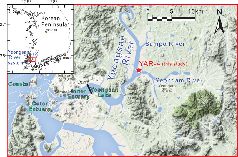
FIGURE 1. Topographic map of the Yeongsan Estuary showing the location of the YAR-4 core site (red star). Inset: location of the Yeongsan River system (blue lines). Maps were obtained from Google Maps. The location of the Yeongsan Estuarine dam is also shown by black bar.

The Yeongsan Estuary has experienced substantial coastal construction within the last 100 years, a dam construction (the Yeongsan Estuarine Dam, drawing boundary between the Inner Estuary and the Yeongsan Lake at present) by 1981, and land reclamation projects during the 1980s, which led to reduction of the estuarine area (e.g., Williams et al., 2014). Prior to the dam construction, tidally influenced environments spanned about 63 km upstream from the dam (Lee et al., 2009). During the land reclamation projects, seawalls/embankments were constructed within the area.

YAR-4 (34.82167 °N, 126.55357 °E; 0.5 m below mean sea level at the top) is a 20-m-long sediment core (inner diameter, ∼74 mm) that was recovered adjacent to the junction of the Yeongam River (also called the Yeongam tributary) and the main channel of the Yeongsan River (Figure 1). Prior to the dam construction the core site would have been below mean sea level and the dam construction actually exposed the core location. The YAR-4 core site has had no tidal influence since the dam construction. The average accumulation rate of sediments around the site is presently estimated at ∼20 mm/yr (Williams et al., 2014). Weathered granite (basement rock) is apparent at the bottom 0.20 m of this core; from a core depth of 19.80 m to the top, various facies of sediments are visible (Figure 2). The sediment descriptions, interpretation of the sedimentary environments, and accelerator–mass spectrometer (AMS) radiocarbon (¹⁴C) age data for this core have been previously documented (Nakanishi et al., 2013), and are briefly described as follows.

FIGURE 2

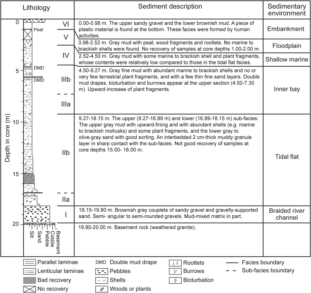
FIGURE 2. Summary of sedimentary characteristics of the YAR04 core documented by Nakanishi et al. (2013), showing columnar lithology, sediment descriptions and inferred sedimentary environments.

Nakanishi et al. (2013) divided the YAR-4 core sediment stratigraphy into six different sedimentary facies units (I, II, III, IV, V, and VI, in Figure 2) based on their analyses, including grain size, color, sedimentary features, and AMS ¹⁴C age data. Units II and III are further subdivided into two subfacies units each, as IIa, IIb, IIIa, and IIIb. Figure 2 presents a summary of the core’s sedimentary characteristics and the interpretation of associated sedimentary environments. Nakanishi et al. (2013) also estimated a number of AMS ¹⁴C ages (i.e., only conventional age estimates, without ¹⁴C calibration) from materials of terrestrial (plants) and marine (shells) origins to evaluate the marine reservoir effects on the sediments. Their results revealed that the shell ¹⁴C ages were older by 0–500 years (i.e., the marine reservoir effects) than the plant ¹⁴C ages.

In the present study, we selected part of the plant ¹⁴C age data from the published age dataset to represent appropriate sediment ages (Table 1; Figure 3) to build up an age–depth relationship for this core and to estimate the sedimentation rates. These ages ranged from 8,130 (±70, 1σ) to 3,760 (±50, 1σ) yr BP in conventional age for units II to V, being converted into calibrated ages from 9,088 (±310, 2σ) to 4,114 (±179, 2σ) cal. yr BP by using the OxCal (version 4.4) calibration program (https://c14.arch.ox.ac.uk/oxcal.html) with the IntCal20 (Reimer et al., 2020). Unit I had no ¹⁴C age determination due to the absence of samples suitable for ¹⁴C dating. Based on these selected data points, we constructed an age-depth model (Figure 3) by using the software “Undatable” (Lougheed and Obrochta, 2019), which ran 100,000 Monte Carlo iterations with setting parameters of xfactor = 0.1 and bootpc = 10 in treating uncertainty (for details about the xfactor, the bootpc, and the modeling, see Lougheed and Obrochta, 2019). This YAR-4 age–depth model indicated several drastic changes in the sedimentation rate, which ranged apparently between 0.4 and >25 mm/yr.

TABLE 1

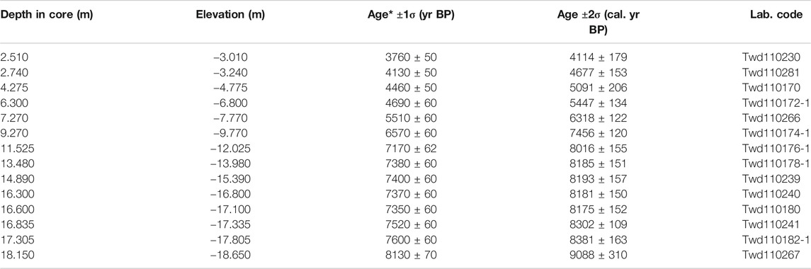
TABLE 1. Accelerator mass spectrometry (AMS) ¹⁴C age data for materials of terrestrial origin (plant fragments) of the YAR-4 core, selected from the dataset of Nakanishi et al. (2013). Age* denotes a conventional age estimate before ¹⁴C calibration reported in Nakanishi et al. (2013). Age (±2σ) in cal. yr BP denotes the calibrated age estimate using the OxCal (version 4.4; https://c14.arch.ox.ac.uk/oxcal.html) and the IntCal20 (Reimer et al., 2020) by this study.

FIGURE 3

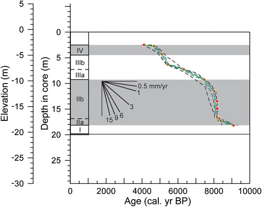
FIGURE 3. Plot of the calibrated ¹⁴C age data that are used for this study (also given in Table 1) with depth in core and elevation, and an age–depth model reconstructed by using the “Undatable” (Lougheed and Obrochta, 2019), with xfactor = 0.1, bootpc = 10, and 10⁵ Monte Carlo iteration runs (see Supplementary Table S6). Each age data point is given by red-filled circle. The age-depth model median is denoted by green line. The 1σ and 2σ uncertainties of the age-depth model are denoted by dashed blues and black lines, respectively. The sedimentary unit divisions (I to VI) are supplementarily shown near the y-axis.

Methods

All of the following subsample preparations and procedures for analyses of sediment particle size, total organic carbon (TOC), and a suite of magnetic properties were conducted at the laboratories of the Korea Institute of Geoscience and Mineral Resources (KIGAM, Republic of Korea). Only microscopic observations were conducted at the Central Research Facilities of Gyeongsang National University (Republic of Korea).

For the split half-core, subsamples for analyses were collected using cylindrical plastic tubes generally at ∼0.04-m intervals and a subsampling thickness of ∼0.02 m from the core depth interval of 3.20–20.00 m. The subsamples were oven-dried at 40 °C for approximately 24 h prior to analyses.

Particle Size and Total Organic Carbon Measurements

The particle size distribution of bulk sediment was analyzed at ∼0.5-m intervals using a Mastersizer 2000 laser analyzer (Malvern Instrument Ltd., United Kingdom) using approximately 300 mg of each dried subsample, after treatment with 35% H₂O₂ and 1 N HCl to dissolve organic matter and biogenic carbonates, respectively, and then with ultrasonic dispersion to facilitate complete disaggregation.

To measure the TOC content of bulk sediment, each subsample was treated with 1 N HCl at approximately 100°C for 1 h and then transferred to a tin combustion cup after rinsing with distilled water. The TOC content was analyzed at ∼0.2-m intervals using a CNS elemental analyzer (vario Micro cube; Elementar, Germany).

Measurements of Magnetic Properties

Magnetic properties were measured using three types of dried subsamples: bulk sediment sealed in a non-magnetic plastic box (volume, 7 cm³), several tens of mg of bulk sediment sealed in a gelatin capsule and capped with glass wool, and several tens of mg of magnetic mineral extracts sealed in a gelatin capsule and capped with glass wool. Each extraction of magnetic minerals was obtained using a hand magnet. The numbers of each type of the subsample prepared were 153, 41, and 31, respectively. The “packed-in-plastic box” bulk subsamples were used in measurements with a MS2B magnetic susceptibility meter (Bartington Instruments Ltd., United Kingdom). Both of the bulk and extracts “packed-in-gelatin capsule” subsamples were used in measurements with a MicroMag Model 3,900 vibrating sample magnetometer (VSM; Princeton Measurements Corp., United States). By using the MS2B magnetic susceptibility meter, volume-specific magnetic susceptibilities with low-frequency (0.47 kHz) and high-frequency (4.7 kHz) (k_LFQ and k_HFQ, respectively) were obtained. By using the VSM, magnetic hysteresis loop measurement, progressive alternating field (AF) demagnetization of isothermal remanent magnetization (IRM), progressive IRM acquisition, and first-order reversal curves (FORCs) measurement were conducted. The MS2B measurements were applied on subsamples at about 0.04–0.10-m intervals, and the VSM measurements were applied on subsamples that were from a limited number of different horizons of the sediment core.

The k_LFQ and k_HFQ of subsample were established by the average of double measurements with the correction for diamagnetic contribution of the plastic box to magnetic susceptibility, which was made by subtracting the average value of measurements of five empty boxes. These allowed us to calculate frequency-dependent susceptibility (k_FD in %) using the following formula: k_FD = (k_LFQ − k_HFQ)/k_LFQ × 100.

Prior to the VSM measurements, the “packed-in-gelatin capsule” subsamples to be measured were weighed to permit calculation of mass-specific values. Each hysteresis loop was measured up to maximum fields of ±0.5 T, and then, after correction for paramagnetic contribution within the loop, saturation magnetization (M_s), saturation remanence (M_rs), and magnetic coercivity (B_c) were calculated. From each hysteresis loop, low-field magnetic susceptibility (χ_lf; total magnetic susceptibility) was calculated from the initial slope and high-field magnetic susceptibility (χ_hf), as a susceptibility estimate of paramagnetic (plus diamagnetic) minerals, was calculated from the high-field slope of the hysteresis loop. Note that for magnetic susceptibilities, k denotes volume-specific susceptibility in SI units (dimensionless), and χ denotes mass-specific susceptibility (m³/kg in SI units). From each progressive AF demagnetization of IRM, the remanence coercivity (B_cr) was determined as the applied field at which the remanence becomes zero. Each progressive IRM acquisition was made until 1 T was reached. Among the IRM acquisition data, IRM obtained at 1 T (IRM_1T; roughly considered as SIRM) was used as a magnetic property in this study. To unmix the magnetic mineral components contributing to the total remanent magnetization, each progressive IRM acquisition dataset was processed using the Max Unmix software (Maxbauer et al., 2016), which obtains the best fit for the total IRM acquisition using the fewest possible components that are characterized by the SIRM, the median field (Bh) at which half of the SIRM is reached, and dispersion (Dp) of its corresponding cumulative lognormal distribution. For each FORC analysis, 232 or 266 FORCs were measured; these FORC data were processed to create a FORC diagram using the FORCinel software (Harrison and Feinberg, 2008) with a smoothing factor of 9 or 10.

Magnetic susceptibility and IRM_1T generally reflect the abundance of the total of magnetic mineral types and ferromagnetic mineral types (refer to ferrimagnetic and antiferromagnetic, in this study), respectively. χ_hf/χ_lf reflects the contribution of paramagnetic components to the total susceptibility. k_FD indicates the contribution to total susceptibility made by viscous superparamagnetic (SP; < ∼30 nm) grains. B_c and B_cr may be used as measures of the relative proportions between low- and high-coercivity ferromagnetic mineral components, with higher values corresponding to higher proportions of high-coercivity minerals. B_cr/B_c, M_rs/M_s and FORC diagram provide information related to grain size distribution, mainly for ferromagnetic minerals.

Electron Microscope Observations

Electron microscopic observations were conducted selectively on bulk sediment subsamples from four horizons of 7.84, 8.70, 13.40, and 15.25 m depth in core, in order to identify existing magnetic minerals, especially low- and intermediate-coercivity minerals. Polished surfaces of the bulk sediment subsamples were observed using a JSM-7610 F field emission scanning electron microscope (FE-SEM, JEOL, Japan) equipped with an energy-dispersive X-ray spectroscopy (EDS). From the observations, back scattered electron images and EDS spectra of magnetic minerals were obtained.

Results and Discussion

Particle Size and Total Organic Carbon for Bulk Sediments

Table 2 and Figure 4 present the results of particle size and TOC analyses of bulk sediment subsamples, and statistics including minimum, maximum, mean and standard deviation values for sedimentary units, and their downcore variation. The mean particle sizes from depths of 3.2–∼14 m was fairly constant at ∼10 μm (fine silt); below a depth of 14 m, the mean size tended to increase with depth, with fluctuations reaching 104 μm (very fine sand) at a depth of 18.70 m. The TOC content was mainly very low (<0.9%); its variation was minor to a depth of ∼14 m, except at 12.50 m, and appeared to be negatively correlated with the mean size variation throughout the entire sediment core.

TABLE 2

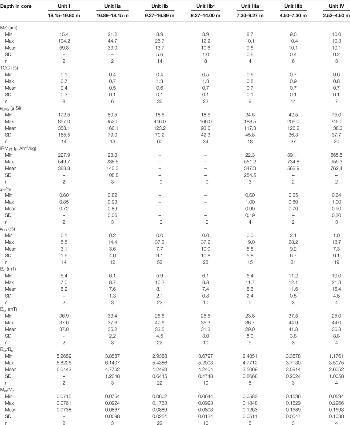
TABLE 2. Summary statistics of mean grain size (MZ), total organic carbon (TOC) content, and various bulk magnetic properties from the YAR04 core sediments (the Yeongsan Estuary). Note that calculations of k_FD statistics were made using only the k_FD values of no less than zero, for convenience with a consideration of the exclusion of unrealistic values presumably due to measurement errors.

FIGURE 4

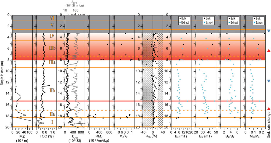
FIGURE 4. Downcore variations in mean grain size (MZ), total organic carbon (TOC) content and various magnetic properties for bulk sediment samples of the YAR-4 core. The magnetic properties shown include bulk magnetic susceptibility (k_LFQ, in both linear and log scale), isothermal remanent magnetization (IRM) intensity imparted at 1 T (IRM_1T), high-field to low-field magnetic susceptibility ratio (χ_hf/χ_lf), frequency-dependent magnetic susceptibility (k_FD), coercive force (B_c), coercivity of remanence (B_cr), ratio of B_cr to B_c (B_cr/B_c), and ratio of saturation remanence to saturation magnetization (M_rs/M_s). In B_c, B_cr, B_cr/B_c, and M_rs/M_s plots, exceptionally, the respective values for magnetic extracts were also shown (assuming their values for the extracts having no significant differences with those for bulk sediments). In the k_FD–depth diagram, the hatched area denotes lack of meaningful k_FD values due to weak signals. Sedimentary unit divisions (I to VI) are shown by orange lines. On the right edge of the figure, the depths at which significant change in sedimentation rate appeared based on the age-depth model (Figure 3) are shown: red triangle denotes increase in sedimentation rate at above the depth, and blue inverse triangle denotes its decrease at above the depth. Gray-shaded area denotes lack of analyzed data.

Downcore Variation in Magnetic Properties

Table 2 and Figure 4 summarize the results of major magnetic property analyses. Table 2 provides summary statistics of the individual magnetic properties including k_LFQ, IRM_1T, χ_hf/χ_lf, k_FD, B_c, B_cr, B_cr/B_c and M_rs/M_s, for the sedimentary units. Examples of the measured and high-field slope corrected hysteresis loops are illustrated in Figure 5. VSM-derived magnetic properties for bulk subsamples were barely detectable due to the weak and quite noisy signals during measurements, such that most of these bulk samples did not produce meaningful values in IRM_1T, χ_hf/χ_lf, B_c, B_cr, B_cr/B_c and M_rs/M_s. Instead, B_c, B_cr, B_cr/B_c and M_rs/M_s were obtained mostly from magnetic extracts of subsamples. We assume that the extract subsamples are representative of the bulk materials for these B_c, B_cr, B_cr/B_c, and M_rs/M_s values. Although there was exactly no horizon where bulk and extract subsamples both were measured for these magnetic property values in this study, it may be supported in part by the fact that, in the interval of 7.90–8.00 m depth in core, their values on bulk and extract subsamples were apparently similar. Downcore variations in these magnetic properties are shown in Figure 4.

FIGURE 5

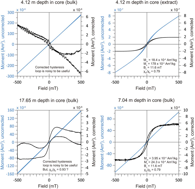
FIGURE 5. Examples of measured (uncorrected) and high-field slope (i.e., paramagnetic contribution) corrected hysteresis loops. The differences between uncorrected and corrected loops indicate substantial non-ferromagnetic (i.e., paramagnetic) contribution in the studied sediments. Note that, for the extract subsample of 17.65 m depth (in core), the corrected loop seems to be less well-constrained so that the hysteresis parameters (M_rs, M_s, and B_c) could not be determinable, but the determined χ_hf/χ_lf seems meaningful.

k_LFQ, which was obtained using the MS2B meter and was volume-corrected for its proper quantification, ranged between 18 and 857 × 10⁻⁶ SI for all analyzed samples, and the means of the respective sedimentary units were from 94 to 358 × 10⁻⁶ SI. Most of the individual values are much lower than 400 × 10⁻⁶ SI. Considerably high values with >400 × 10⁻⁶ SI are limited in the intervals corresponding to the gravel-rich (around 16.9 and 18.15–19.80 m depth) and the basement rock (19.80–20.00 m depth) lithology. In the downcore k_LFQ variation, there are a number of significant susceptibility minima representing lowering by at most 65–80% of the overall mean (for example, at depths of approximately 8.70, 9.70, and 12.20–12.50 m). There are some datasets of k values from Holocene sediment cores at around the studied region, making available for comparison with our data: in the western coastal estuaries of South Korea, ∼0.1–0.2 × 10⁻⁶ SI (Gyeonggi Bay, Moon et al., 2018), and ∼2–12 × 10⁻⁶ SI (Namyang Bay, Lim et al., 2004); in the southern coast of South Korea, ∼300–650 × 10⁻⁶ SI (Geoje Island, Lim et al., 2014), and ∼50–400 × 10⁻⁶ SI (Yeoja Bay, Lim et al., 2015); in the inner shelf of the southwestern East China Sea, ∼200–250 × 10⁻⁶ SI (Zheng et al., 2010), and ∼100–220 × 10⁻⁶ SI (Zheng et al., 2011). The extremely low k values in the Gyeonggi Bay and the Namyang Bay may result from locally particular layers (e.g., organic-rich layer, siderite-rich layer). Besides this, the ranges of k values of the previous studies are comparable to that for the YAR-4 core. However, this comparison should be taken care because it is not straightforward to identify whether or not these previously reported k values were after applying volume corrections (including calibrations of the prepared sample volume and the sensor of instruments used).

Values of mass-specific susceptibility (χ) can be more proper in comparison with previously reported datasets. Unfortunately, our analyzed subsamples were not weighed, thereby not permitting to determine accurately χ values for the same subsamples. Nevertheless, the χ values could be approximated by converting the aforementioned volume-specific susceptibility (k) values, using a mean density of 1.17 g/cm³ and a mean water content of 71.3 wt% for wet surface sediments in the Yeongsan Lake (An et al., 2019). Assuming the water density of 1.00 g/cm³ and that the porosity of the studied sediments (silt-dominant, shallow depths) was little varied through the whole core (i.e., negligible porosity variation for shallow depths; e.g., Bahr et al., 2001), a mean value in dry density of the studied sediment samples could be approximated to 2.03 g/cm³ (considered as a maximal value). Accordingly, the individual k_LFQ values could be converted to the mass-specific susceptibility (χ_LFQ) values in the range of ∼0.9–∼42 × 10⁻⁸ m³/kg, and the χ_LFQ values were generally in the order of 5–10 × 10⁻⁸ m³/kg. This range of mass magnetic susceptibility values is similar in the order of magnitude of or slightly lower than those of Holocene sediment cores of the Yangtze delta area (e.g., ∼10–90 × 10⁻⁸ m³/kg, Chen et al., 2015; ∼35–130 × 10⁻⁸ m³/kg, Pan et al., 2017), shallow shelf sediment cores with anoxic environments in the Korea Strait and off the west coast of the Korean Peninsula (∼18 × 10⁻⁸ m³/kg, Liu et al., 2004; ∼14 × 10⁻⁸ m³/kg, Liu et al., 2005).

Individual IRM_1T values for bulk sediments ranged between 22 and 959 × 10⁻⁶ Am²/kg. These values are significantly lower than those observed in estuarine and shallow shelf sediments of the Korea Strait, the western Yellow Sea and the East China Sea, e.g., ∼200–4,500 × 10⁻⁶ Am²/kg (Liu et al., 2004); ∼150–30,000 × 10⁻⁶ Am²/kg (Chen et al., 2015); ∼2,400–6,100 × 10⁻⁶ Am²/kg (Pan et al., 2017). The individual IRM_1T values exhibited an apparent decreasing trend with depth to ∼8 m, and we observed roughly similar values in the two intervals at depths of 7–8 and 17.5–18.5 m.

χ_hf/χ_lf values ranged between ∼0.6 and 1.0, indicating significantly larger paramagnetic contributions than ferromagnetic contributions (see also Figure 5), presumably in most of the sampled sediments.

The k_FD values, with exception of negative values, ranged between 0.0 and 37.2%, of which values >20% may not be reliable due to weak susceptibility signals. The mean values for respective sedimentary units were approximately between 3 and 10%, indicative of, in general, somewhat or considerable SP contributions in the sediments. Due to concern from the mixing with untrustworthy data, we did not used the k_FD data in discussing on its detailed variability in association with the diagenetic, sea-level, and climate effects.

Individual B_c, B_cr, B_cr/B_c, and M_rs/M_s values ranged between 5 and 21 mT, between 24 and 45 mT, between 2.44 and 5.20, and between 0.06 and 0.30, respectively. Downcore variation in B_c and M_rs/M_s created an apparent division into two zones at a depth of ∼8 m, with relatively constant low values in the lower zone and constant higher values in the upper zone. Interestingly, downcore variation in B_c, B_cr, and M_rs/M_s shared a distinct, drastic increase in the respective parameter at depths of 15.25 m and 7.84–7.96 m. At depths above 7.84 m, such high values were sustained after this abrupt increase, whereas low values appeared the same as the surrounding data points at depths immediately above and below 15.25 m (i.e., 15.05 and 15.45 m).

Figure 6 presents plots of k_LFQ vs. the other magnetic properties examined in this study, to assess possible relationships with k_LFQ. Generally, we observed no or very week correlation with k_LFQ, but B_cr had a moderate positive correlation with k_LFQ. This implies complexity of mineral magnetic factors controlling k_LFQ (e.g., content of paramagnetic minerals, content, composition ratio, and grain size of ferromagnetic minerals).

FIGURE 6

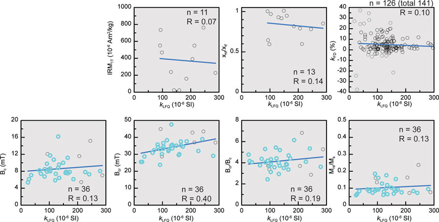
FIGURE 6. Biplots of k_LFQ vs. each of several other magnetic properties (IRM_1T, χ_hf/χ_lf, k_FD, B_c, B_cr, B_cr/B_c and M_rs/M_s). k_LFQ all were from bulk sediment samples. For the respective biplots, a fit line and its corresponding correlation coefficient (R) is provided. Black (Cyan) circles denote the data where the magnetic property values were obtained from the bulk (extract) samples. For the k_LFQ vs. k_FD plot, the data that were in out of the range between −5 and 20 in k_FD (gray circles), being regarded less reliable, were excluded when consdiering the correlation degree between k_LFQ and k_FD.

Magnetic Mineralogy and Granulometry from Magnetic Measurements and Scanning Electron Microscope Observations

SEM observations provided back scattered electron images and EDS spectra of magnetic minerals in the sediments (Figures 7 and Supplementary Figure S1). From the observations, pyrite (FeS₂), greigite (Fe₃S₄), and (titano)magnetite are identified. It is found that pyrite is ubiquitous and has the most dominance in magnetic minerals in all analyzed bulk sediment samples (i.e., 7.84, 8.70, 13.40, and 15.25 m depth in core; Figures 7A and Supplementary Figure S1). The pyrite exists as framboidal aggregates and separated euhedral crystals with variable sizes in the sediment matrix, in the vicinity of silicates, and in the voids of the matrix (Figures 7A,C, and Supplementary Figure S1). The pyrite grains forming the framboids are much smaller (roughly <0.3 μm in maximal length) than the separated euhedral ones (roughly 0.5‒<10 μm in maximal length). These pyrite grains all are considered to be of post-depositional authigenic origin. The (titano)magnetite grains occur in the matrix, their shape is angular, and their size is between several microns and more than 10 microns (Figure 7B). Such characteristics of the (titano)magnetite grains allows us to interpret it as detrital origin. The occurrence of (titano)magnetite grains is much less frequent than the pyrite grains. No sub-micron to nano-size (titano)magnetite grains are found. The greigite occurs in the shape of framboids or irregular aggregates within and around aggregates of pyrite crystals, and their size is much smaller (nano-scale; presumably in the SP to stable SD size range) than the pyrite grains (Figures 7C,D). The gregite grains are interpreted as being of post-depositional origin.

FIGURE 7

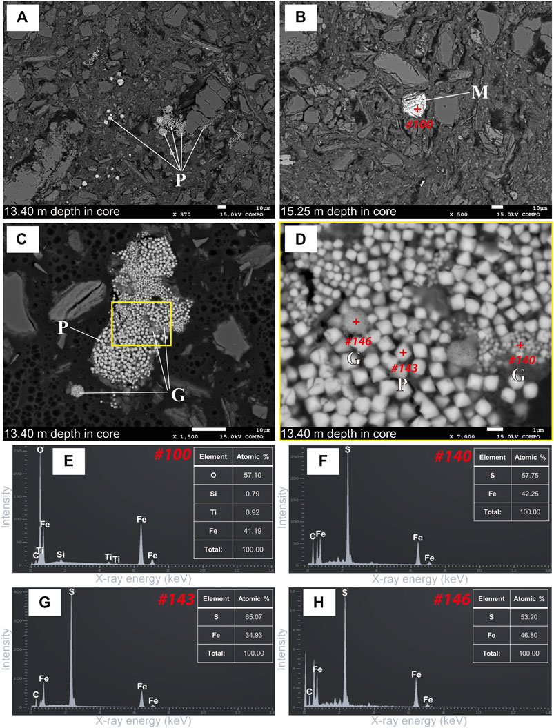
FIGURE 7. BSE images and X-ray EDS spectra of magnetic minerals presented in bulk sediments from the YAR-4 core. (A) Euhedral pyrite grains, and framboidal and irregular pyrite aggregates (labeled P) in silicate/clay-dominated matrix from the 13.40 m depth sediment sample. (B) Titanomagnetite grain (labeled M) in silicate/clay-dominated matrix from the 15.25 m depth sediment sample, being probably of detrital origin. Red cross symbol indicates the target point where EDS analysis was conducted. (C) Polyframboidal aggregates of both pyrite (labeled P) and greigite (labeled G) grains from the 13.40 m depth sediment sample. (D) Zoom-in view of (C). Ultra-fine-grained gregite aggregates (finer than the surrounding pyrite grains) within the aggregates of pyrite crystals of variable sizes. The greigite grains are roughly bimodal in size. Red cross symbols are the same as in (B). (E–H) EDS spectra of (Ti-poor) titanomagnetite (Fe_3-xTi_xO₄; x = ∼0.1) shown in (B) and pyrite and greigites shown in (D), respectively, with element compositions in atomic %. Ideal atomic % is given approximately Fe = 33, and S = 67 for pyrite (FeS₂), and approximately Fe = 43, S = 57 for greigite (Fe₃S₄). The carbon (C) signal of EDS originates from the carbon coating of the sample thin section in preparation for the SEM observation.

As described in Downcore Variation in Magnetic Properties Section, paramagnetic minerals, rather than ferromagnetic minerals, appear to control the bulk magnetic properties (such as bulk magnetic susceptibility) of the studied sediments. Candidates for these major paramagnetic minerals are common iron-bearing clay minerals with detrital origin, pyrite, iron monosulfide (mackinawite, FeS), and siderite (FeCO₃) of diagenetic (authigenic) origin in estuarine sediments. The gray or olive-gray colors of most of the studied sediments may be associated with abundant pyrite, which is consistent with the SEM observations. Several studies of other Holocene tidal flat sediments on the west coast of South Korea have reported authigenic siderites that were formed by early diagenesis during the Holocene through interactions with freshwater (Khim et al., 2000; Choi et al., 2003; Lim et al., 2004). Lim et al. (2004) also documented the siderite-abundant sediment interval (the unit T1 in their study) that was characterized by reddish- or yellow-brown (10 YR 5/4) massive mud and 10–12 × 10⁻⁶ SI in bulk magnetic susceptibility.

Meanwhile, ferromagnetic minerals in the studied sediments also contribute to magnetic property variation, and leave meaningful signals. The IRM component unmixing analyses revealed occurrence of magnetic mineral components with different coercivity spectra from the total IRM. Figure 8 presents the results of unmixed magnetic mineral components and their relative contributions in IRM unmixing analyses from selective stratigraphic levels in different sedimentary units (13 subsamples). These results indicate the presence of at least three components (in the upper part of the core, four) throughout the entire analyzed sediments: component 1, with low Bh (23–31 mT); component 2, with intermediate Bh (mainly 50–71 mT); component 3, with high Bh (129–399 mT); and occasionally component 4, with high Bh (>1,000 mT). The components 1, 3, and 4 were interpreted as pseudo-single-domain (PSD) and/or multi-domain (MD) magnetite (Fe₃O₄; ferrimagnetic), probably of detrital origin; hematite (α-Fe₂O₃; antiferromagnetic); and goethite (α-FeOOH; antiferromagnetic), respectively (e.g., Maxbauer et al., 2016). Note that the components 3 and 4 having high-coercivity spectra were not recognized in the SEM observations of this study. The component 2 possibly imply greigite (Fe₃S₄; ferrimagnetic) due to the similar remanence coercivity values for greigite-bearing sediments (mainly 60–95 mT, but 37–98 mT for a wider range; Roberts, 1995; Snowball, 1997; Peters and Dekkers, 2003). This can be supported by the occurrence of ultra-fine greigite grains in SEM observation. We find that the relative contributions of these components differ at different depths, but generally the contribution of the components 1 and 2 dominates throughout the sediments.

FIGURE 8

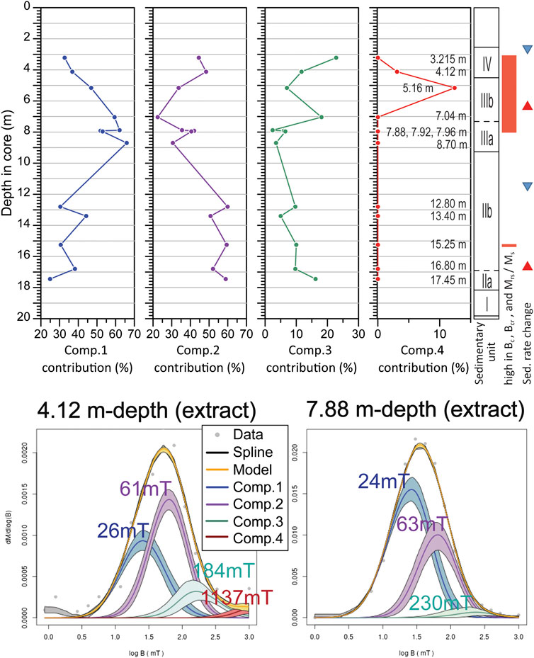
FIGURE 8. Two examples of IRM component unmixing analyss results by using Maxbauer et al. (2016)(lower) and relative contributions of the unmixed magnetic mineral components for samples at different depths (upper; n = 13). In the figures of the lower panel, the mean coercivity (Bh) of each unmixed component (comp.) is labeled. On the right hand of the upper panel figure, the division of sedimentary units (the same as in Figure 2), the intervals with high values in B_c, B_cr, and M_rs/M_s (the same as in Figure 4), and the depths above which the sedimentation rate changes significantly (the same as identified in Figure 3; the triangles are the same as in Figure 4) are supplementarily shown.

Peters and Thompson (1998) discriminated between different magnetic minerals by constraining the typical ranges for the respective minerals in a biplot of IRM_1T/χ_lf vs. B_cr. As shown in Figure 9, part of our YAR-4 data (n = 11) did not fall into the range of (titano-)magnetite or greigite, but instead were superimposed partly on the range of the A5 sediments of New Jersey Miocene clays reported in Nilsson et al. (2013) who interpreted them as mixtures of (titano-)magnetite and greigite. It might be also possible that the plotted range of our data was influenced partly by the presence of hematite (and occasionally goethite).

FIGURE 9

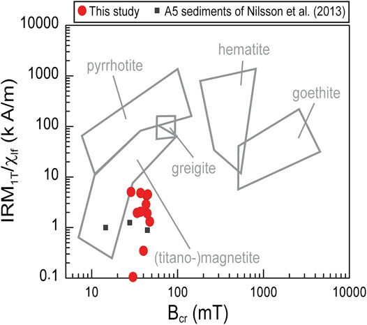
FIGURE 9. Biplot of IRM_1T/χ_lf vs. B_cr for the YAR-4 core sediments (red circles; n = 11), with typical ranges (gray boxes) of the magnetic parameters for different minerals proposed by Peters and Thompson (1998) and data for the A5 sediments reported by Nilsson et al. (2013) (black squares).

Figure 10 presents FORC diagrams for four selective subsamples at different depths to provide additional information in terms of magnetic mineralogy and its domain state (also associated to grain size distribution of the magnetic mineral assemblage). Although the analyzed FORC diagrams are somewhat noisy, probably due to low concentrations of magnetic minerals, they still offer meaningful information. The FORC diagram for the 5.16-m-depth subsample had a B_c peak at ∼10 mT and vertically suppressed divergence in contour distribution that was partly closed but the others intersected the B_u axis. This pattern resembles the FORC diagrams of Figures 6A,B (Nankai Trough drilling sediments) in Kars and Kodama (2015) who interpreted them as the presence of single-domain (SD) to PSD magnetite. Dominant appearance of the magnetite-related signals for the subsample can be correlated to the most relative contribution of component 1 indicated by the IRM unmixing (Figure 8). The 7.84-m-depth FORC diagram had strong B_c (∼10 mT) and weaker B_c (∼27 mT) peaks, a closed but vertically spreading contour distribution that also elongated to higher coercivities along the B_c axis, and a negative region distributed along the lower half of the B_u axis. This pattern might be indicative of the presence of PSD greigite (e.g., Figure 5 in Roberts et al., 2011) in addition to SD-to-PSD magnetite. The 13.40-m-depth FORC diagram contained two B_c peaks at ∼10 mT and near the origin. Its contours were spreading vertically wider at lower B_c values, and were not closed but intersected the B_u axis, being vertically stretched along the lower half of the B_u axis. At low B_c values, the contours were also distended diagonally downward. Such features possibly indicate the presence of PSD detrital magnetite (Roberts et al., 2018a) and SP magnetite or another magnetic mineral (Roberts et al., 2000). In this case, the SP-related feature could be interpreted to originate from ultra-fine greigite grains as indicated by the SEM observations. The 15.25-m-depth FORC contours had a B_c peak at ∼18 mT, and larger elongation to higher coercivities along the B_c axis. The dense contour concentration up to at higher B_c values relative to the other samples might be related to the higher component 2 content at the 15.25-m-depth indicated by the IRM unmixing result (Figure 8). The contours had a vertical spreading pattern that got wider gradually as B_c decreased toward the origin, and were partly closed but the others intersected the B_u axis. The contour pattern is interpreted to indicate the presence of SD and PSD grains (e.g., Roberts et al., 2000). Overall, the FORC contour patterns tell us that the 13.40-m-depth sample showed predominance of (relatively large) PSD and SP ferromagnetic grains, but the other three samples showed predominance of SD to (relatively small) PSD grains. The SP grains was interpreted as being of diagenetic greigite.

FIGURE 10

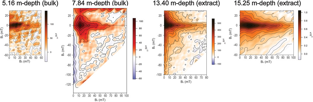
FIGURE 10. First-order reversal curve (FORC) diagrams for four subsamples at different depths.

Also, none of the FORC diagrams shown had such a contour pattern of central ridge with mainly suppressed vertical spreading, which is indicative of the presence of biogenic magnetite of authigenic origin (Roberts et al., 2012). Thus, it is interpreted that biogenic magnetite cannot be a candidate for the middle-coercivity mineral component indicated by the IRM component unmixing (the component 2 in Figure 8).

Figure 11 presents our hysteresis parameter ratio data (M_rs/M_s and B_cr/B_c) on a Day diagram (Day et al., 1977). These data mostly fall in the PSD region of Dunlop (2002a), and almost all of them are distributed in the region between the SD + MD 3 and the SD + SP (10 nm) mixing lines of Dunlop (2002a) and Dunlop (2002b). As pointed out by Roberts et al. (2018b), such Day diagram result should be taken with care in diagnosing domain state (or grain size) particularly for mixed assemblage of multiple magnetic minerals as presented in this study. Nevertheless, it can be useful to recognize downcore relative variation in magnetic granulometric trend. The data at shallow depths down to 7.92 m fall within a relatively restricted region that is at the up left-hand side of the data distribution, whereas the others at deeper than 7.92 m, except the 15.25 m one, are distributed within the down right-hand region with low values in M_rs/M_s and B_cr/B_c. With a comprehensive view from the IRM unmixing and FORC results, such variation on Day diagram is interpreted to be caused mainly by difference in grain size distribution of ferromagnetic minerals, rather than by variation in mineralogical composition. Then it is interpreted that samples being plotted at more toward the up left-hand side on the Day diagram have more abundant ferromagnetic grains with close to stable SD to SD‒PSD boundary in size but less SP grains, relative to the down right-hand plotted samples.

FIGURE 11

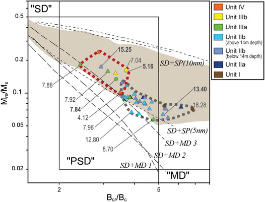
FIGURE 11. Day plot of our YAR-4 core sediment data (n = 37) at different depths and sedimentary units. Circle and triangle symbols denotes the data measured from bulk and extract samples, respectively. Some data are labeled using the “depth in core” in meter, among which the data labeled in bold denote those where the associated FORC diagrams are provided in Figure 10. Single-domain (SD), pseudo-single-domain (PSD), and multi-domain (MD) boundaries, trend curves 1, 2, and 3 for SD + MD mixtures of magnetite and trend curves for SD + SP with 5-nm and SD + SP with 10-nm mixtures of magnetite were drawn by Dunlop (2002a), Dunlop (2002b). Color-shaded region represents a typical range for SD + SP mixtures of greigite indicated by Roberts et al. (2011). Division of the data into two groups by dashed enclosed lines was based on ranges of the B_c, B_cr, and M_rs/M_s values (see text for details).

Diagenetic Effects on Downcore Variation in Magnetic Properties

In a wide range of sediments, but especially marine sediments from shallow continental shelf to deep-sea environments, early post-depositional diagenesis generally causes selective dissolution of relatively coarse micron-size detrital iron oxides (e.g., magnetite, hematite), and authigenic formation and growth of nano-to sub-micron-size magnetic minerals (e.g., pyrite, greigite, siderite), leading to systematic changes in the concentration and grain size of magnetic minerals with depth (e.g., Karlin and Levi, 1983; Liu et al., 2004; Rowan et al., 2009; Hatfield, 2014; Roberts, 2015). Due to the degradation of primary magnetic signals associated with paleoenvironmental changes, identifying and understanding the effects of such early diagenesis on magnetic minerals is crucial for interpreting environmental magnetic records (Snowball and Thompson, 1990; Verosub and Roberts, 1995; Liu et al., 2004; Demory et al., 2005).

Using our results from the depth interval of 3.2–13.9 m, at which sediment mean particle sizes and TOC contents vary little, we attempted to assess relatively straightforwardly early diagenetic effects on downcore variations in magnetic properties in the YAR-4 core.

In a general model for sediment cores influenced by early diagenesis, downcore variation exhibits significantly decreasing magnetic susceptibility with increasing depth in the suboxic zone (below the top shallow sediments (oxic zone) down to the suboxic–sulfidic (anoxic) boundary) and relatively constant low-susceptibility values at depths below the suboxic–sulfidic boundary, under anoxic zones. The magnetic susceptibility range in the 3.2–13.9 m depth interval of the core YAR-4 was similar in the order of magnitude of those observed in anoxic environments of coastal and shallow shelf sediment cores around South Korea and east China (Liu et al., 2004; Liu et al., 2005; Chen et al., 2015; Pan et al., 2017; see also Downcore Variation in Magnetic Properties Section). This result implies that the target interval of the YAR-4 sediments experienced considerable early reductive diagenesis under anoxic conditions, causing considerable dissolution of detrital magnetic minerals. It is apparently in agreement with the current anoxic conditions at depths below 0.03 m, where methane concentrations are higher, at a site in Yeongsan Lake (An et al., 2019). This suggestion is also consistent with the widespread presence of the middle-coercivity component (component 2 in Figure 8), i.e., greigite (see Magnetic Mineralogy and Granulometry from Magnetic Measurements and Scanning Electron Microscope Observations Section), which is a typical authigenic iron mineral, in addition to pyrite and iron monosulfide, which are generated in the sulfate–methane transition zone (SMTZ) (Roberts, 2015).

Rowan et al. (2009) identified downcore variations producing counterclockwise loop trends in Day diagram from marine sediment cores around the world (Figure 9 of Rowan et al., 2009). They ascribed the systematic trends to the superposition of spatio-temporally progressive diagenetic changes of magnetic minerals. This changes include progressive reductive dissolution where finer pre-existing ferromagnetic grains (mostly detrital magnetite) preferentially dissolve to leave a coarser assemblage, and progressive sulfidization resulting in SP greigite nucleation and its progressive growth into the SD size range. The trends occur as the result of magnetic property combinations between survived coarse detrital grains and SP to SD authigenic greigite grains. The looping trend and the YAR-4 downcore variation in Day diagram (Figure 11) apparently share a similar pattern in part, but visible difference between them exists. The whole analyzed interval of the YAR-4 core should be correlated to the “zone 3” of the downcore magnetic property profile shown in Figures 2, 3 of Rowan et al. (2009), based on being the low magnetic susceptibility values throughout the analyzed interval (Figure 4). However, the YAR-4 data in Day diagram lie within a wider B_cr/B_c range, being stretched toward the down right-hand region, than those of the “zone 3” (Rowan et al., 2009). Given this, the YAR-4 downcore variation is inferred to contain more complicated diagenetic effects than those indicated by Rowan et al. (2009) and/or possibly other effects caused by changes in depositional condition.

Magnetic mineral diagenesis is also generally thought to be controlled by depositional conditions, that is, mainly TOC and sedimentation rate (e.g., Hesse and Stolz, 1999). Changes in TOC and sedimentation rate often produce non-steady-state early diagenesis, where diagenetic reactions change with depth as the depositional conditions change (e.g., Thomson et al., 1984; Robinson et al., 2000; Emirog̃lu et al., 2004; Fu et al., 2008; Roberts, 2015). If magnetic property variations of the 3.2–13.9 m depth interval of the YAR-4 core are further ascribed to such non-steady-state diagenesis, the YAR-4 downcore variations should be associated with changes in sedimentation rate because it is expected that the constant low TOC contents throughout the YAR-4 core would bring minimal or negligible effects. Riedinger et al. (2005) documented distinct minima in magnetic susceptibility within a distinct sediment interval, and interpreted them to result from a drastic change in sedimentation rate, which resulted in a fixation of the SMTZ at a specific depth causing substantial change of pre-existing abundant iron (oxyhydr)oxides to iron sulfides. Zheng et al. (2011) proposed that drastic changes in sedimentation rate resulted in vertical shifts of the SMTZ, of which each SMTZ eventually exhibited low magnetic susceptibility, high coercivity, and significant paramagnetic contribution as a result of dissolution of pre-existing detrital magnetite and hematite but strong resistance to the dissolution for hematite relative to magnetite, and their replacement mainly by paramagnetic pyrite. Abrajevitch and Kodama (2011) reported a relationship among mineral magnetic features, i.e., low magnetic susceptibility, coarsening of detrital magnetic grains (e.g., magnetite), increasing relative abundance of hematite, and decreasing relative abundance of goethite during periods with low sedimentation rate (i.e., sea-level highstand, in the case).

Indeed, the YAR-4 core appears to record at least four drastic changes in sedimentation rate and three distinct intervals with relatively low sedimentation rate, based on our age–depth model (Figure 3). However, none of the relations between magnetic properties such as those identified in the above-stated previous studies are identified in the YAR-4 core (see e.g., Figures 4, 8). We thus infer that, in addition to the above-discussed possible diagenetic effects, additional effect(s) caused by another factor(s) should be contained in the downcore magnetic property variations for the YAR-4 core, and speculate the possible presence of certain paleoenvironmental change(s) or even less-known diagenetic processes linked to that (in similar manner as reported in e.g., Larrasoaña et al., 2003, Blanchet et al., 2009, and the review of Roberts, 2015) for the YAR-4 site as the additional controlling factor(s).

Searching for Magnetic Property Features Associated With Paleoenvironmental Changes

Sedimentation in the studied YAR-4 site during the Holocene would have been considerably influenced by sea-level change and hydrologic events that are regarded as closely associated with regional climate changes such as the ENSO activity, the EAM, and the HCO. Accordingly, types, concentration, and grain size distribution of the contained magnetic minerals would change through time, at least partly in response to the sea-level change and/or regional climate changes. Based on our age-depth model (Figure 3), the YAR-4 record of magnetic property variabilities presented in this study covers a period of approximately 4,800–9,000 cal. yr BP (Supplementary Figures S2, S3 and S4). In order to search for magnetic property proxies for paleoenvironmental changes, we compare temporal variations between some of the obtained magnetic properties (we choose k_LFQ, B_c, B_cr, M_rs/M_s, and each of IRM-unmix components for this) and proxy indicating the change in sea-level (Lee and Chang, 2015; Song et al., 2018), the ENSO activity (Moy et al., 2002), the summer EAM (Dykoski et al., 2005), and the HCO with the 8.2 ka cooling event (Park et al., 2019) around the Korean Peninsula, respectively (Figure 12, Supplementary Figures S2, S3 and S4).

FIGURE 12

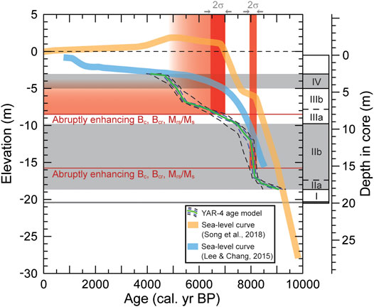
FIGURE 12. Comparison of our age-depth model for the YAR-4 core with two different suggested sea-level curves for the western coast of South Korea (Lee and Chang, 2015; Song et al., 2018). HBBM intervals (characterized by subtantially high B_c, B_cr, and M_rs/M_s values) and their corresponding ages are indicated by red lines and red shaded boxes. The YAR-4 age-depth model curve with the uncertainties are the same as in Figure 3. Sedimentary unit divisions are also supplementarily shown.

In advance of getting to the main discussion, we would like to mention that the use of only initial bulk magnetic susceptibility without detailed additional information about constituent magnetic minerals in interpreting a certain paleoenvironment change (as the same manner utilized in previous studies for Korea with similar purposes to this study) appears to be imprudent, given the k_LFQ values that were substantially influenced by complicated magnetic mineral diagenesis as in the studied case.

Comparisons With El Niño Southern Oscillation Activity, Summer Eastern Asian Monsoon, and Holocene Climate Optimum

Moy et al. (2002) presented a record of red color intensity variability through the Holocene as a proxy representing the ENSO activity variability from a sediment core of the lake Laguna Pallcacocha in the southern Ecuadorian Andes. There exist three extremely high peaks in ENSO activity during ∼4,800–9,000 cal. yr BP (∼4,750–5,000, ∼5,900–6,000, and ∼7,900–8,000 cal. yr BP; green shaded regions in Supplementary Figure S2), and such ENSO peaks are being considered to be related to high frequency and magnitude of flooding or freshwater input from inland at least in the southern part of the Korean Peninsula (Lim et al., 2017, Lim et al., 2019). However, we did not find any of our magnetic property variability data that could be well correlated to those ENSO peaks (Supplementary Figure S2). This implies no or, if any, meager regulation by extreme short-term hydrologic events (also associated with ENSO activity) on the magnetic property variabilities in the YAR-4 site.

The oxygen isotope ratio variability from the Dongge Cave in the South China by Dykoski et al. (2005), adopted worldwide as representative of the summer EAM variability, seems to have similarity partly in centennial (short-term excursion; blue shaded regions shown in Supplementary Figure S3) and millennial (long-term trend; intervals between blue shaded individuals in Supplementary Figure S3) scales to our B_c, B_cr, and M_rs/M_s variabilities (Supplementary Figure S3). It shows apparently a relationship of low B_c, B_cr, and M_rs/M_s values with strong summer EAM. Strong summer EAM generally accompany high accumulation of rainfall precipitation that leads to high terrestrial material input, which can be possibly accompanied with increasing concentration and grain size of detrital magnetic minerals (e.g., magnetite). If it can be assumed that the low B_c, B_cr, and M_rs/M_s values were carried mainly by increasing grain size of detrital magnetite for the YAR-4 sediments, these magnetic properties can be dealt as summer EAM proxies. According to this inference, strong summer EAM conditions should be favorable for coarsening of detrital magnetite, via controlling the local hydraulic condition around the studied area. On the other hand, if so, lowering B_c, B_cr, and M_rs/M_s values should occur at the periods with extremely high ENSO peak (∼4,750–5,000, ∼5,900–6,000, and ∼7,900–8,000 cal. yr BP), through a similar process occurred in strong summer EAM periods with enhanced rainfall frequency and magnitude. However, such relationship appears not visible (Supplementary Figure S2). Therefore, we interpret that such potential hydraulic effect in relation to detrital magnetite grain size does not govern, but may control partly, the B_c, B_cr, and M_rs/M_s variabilities.

Additionally, the HCO period and the 8.2 ka (thousand years ago) abrupt cooling event are also the major phenomena of climate change during the Holocene. The HCO is a warm and humid period with relatively high precipitation, and occurred during ∼4,800–7,600 cal. yr BP for the southern Korean Peninsula (Park et al., 2019; cf., ∼5,100–8,200 cal. yr BP, a calibrated age range in this study with the OxCal and IntCal20 from ∼4,500 to 7,400 years BP in uncalibrated age originally reported by Yang et al., 2008, or ∼5,000–6,300 cal. yr BP by Nahm and Hong, 2014). The 8.2 ka event is a short-term climate excursion to cold and dry condition at ∼8,200 cal. yr BP, and has been identified also in South Korea (Park et al., 2018; Park et al., 2019). It might be good to look at the high (detrital) magnetite relevant abundance (i.e., the IRM-unmixed component 1 contribution) with less greigite relevant abundance (i.e., the IRM-unmixed component 2 contribution) during the HCO period, and vice versa around the 8.2 ka event (Supplementary Figure S4). Blanchet et al. (2009) reported that large flood deposits and glacial deposits are favorable for preservation of diagenetic greigite, and interpreted it to be related to dominance of reactive iron over organic matter and/or HS⁻, i.e., enrichment in terrigenous sediments. According to this, it might be possible that the 8.2 ka cooling triggered relatively enhanced greigite preservation through the early diagenetic process at the studied YAR-4 site. This potential relationship will be worth being tested further in future investigations with more high-resolution magnetic analyses and the use of multiple cores at different sites.

Possible Magnetic Response to Abrupt Drop in the Rate of Sea-Level Rise

Many sea-level change curves have been suggested for the western coast of South Korea during the Holocene (e.g., Bloom and Park, 1985; Hwang et al., 1997; Chough et al., 2004; Lee et al., 2008; Lee and Chang, 2015; Song et al., 2018); however, no consensus has been reached (cf. the review by Choi, 2018). A major discrepancy among them would be the sea level relative to the present mean sea level (MSL) and its change pattern since ∼7,000 cal. yr BP: One group of the sea-level curves depicts that the sea level always was lower than the present MSL and continued a gradual rising toward the present MSL (e.g., Bloom and Park, 1985; Chough et al., 2004; Lee and Chang, 2015), whereas another group suggests a sea-level highstand (higher sea-level relative to the present MSL) during ∼4,000–7,000 cal. yr BP followed by a sea-level drop toward the present MSL (e.g., Hwang et al., 1997; Song et al., 2018). Unfortunately, the sedimentary characteristics and our age-depth model of the YAR-4 core (Figures 2, 12) independently do not allow to fully support one of the two different groups of suggested sea-level curves.

In any case, most suggested sea-level curves of these previous studies depict a drop in the rate of sea-level rise broadly at around 7,000 cal. yr BP. Besides this, the sea-level curve of Song et al. (2018) depicts an additional drastic drop in the sea-level rise rate at ∼8,200 cal. yr BP, then shortly followed by an increase of this rate again, inferring formation of a concomitant short-term slowstand/stillstand (Figure 12). The existence of such “stepped” change in sea-level rise rate as indicated by Song et al. (2018) is being identified even in more recent studies (e.g., Tanabe, 2020). It also would be good to mention that attempts of the west coast sea-level reconstruction during the period back to prior to 8,000 cal. yr BP were rare in among the suggested sea-level curves (cf. Figure 1A in Choi, 2018). Lee and Chang (2015) generated the curve by fitting to the sea-level proxy data that were scarce but highly scattered in the sea-level value during prior to ∼7,800 cal. yr BP (Figure 2 of Lee and Chang, 2015). This may be the reason why the ∼8.2 ka potential drop in the rate of sea-level rise does not appear in the curve of Lee and Chang (2015) (and other previous studies depicting similar curves).

For the YAR-4 core, one remarkable, first-order magnetic feature is the abrupt increases in B_c, B_cr and M_rs/M_s (hereafter referred to as “HBBM feature”) observed at depths of 15.25 and 7.84–7.96 m with their persistent high values at depths shallower than 7.84 m (Figure 4), corresponding to ∼8,100 cal. yr BP and since ∼6,700 cal. yr BP in inferred age (Figure 3; Supplementary Table S6). This observation seems not to be fully explained by solely the sulfidization-dominated diagenetic processes (even if sedimentation rate variability were considered) or correlated well with any of the ENSO activity variability (linked to the local hydrologic events), the summer EAM variability, and the HCO period, as interpreted above. Instead, the respective ages of the two abrupt B_c, B_cr, and M_rs/M_s increases are well coincident with those at which the rate of sea-level rise started to decrease suddenly according to the Song et al. (2018) sea-level curve, given the intrinsic uncertainty of the age-depth model construction (Figures 3, 12; Supplementary Table S6). These concordance allows us to infer that the HBBM feature is strongly related to change of the sea-level rise rate and possibly, sea-level stillstand/slowstand and highstand. The apparent absence of HBBM feature at the old stillstand/slowstand (Figure 12) possibly might be attributed to its short-lived period.

It is worthwhile to discuss and constrain concerning possible mechanism to explain the relation between the change of the sea-level rise rate and the HBBM magnetic feature. A possible major factor enhancing B_c and B_cr could be among increasing relative abundance of hematite and goethite, increasing relative abundance of greigite, and decreasing relative abundance of detrital magnetite, or a combination of them. However, no similar characteristic concerning relative abundance of ferromagnetic minerals between the HBBM intervals (Figure 8; see also Magnetic Mineralogy and Granulometry from Magnetic Measurements and Scanning Electron Microscope Observations Section) allows us to conclude its less probability of being major factor leading to enhancing B_c and B_cr. It, however, would like to be mentioned that, within the 3.21–7.04 m depth interval, there are decreasing magnetite with increasing more high-coercivity minerals in relative abundance, which may be attributable at least partly to the HBBM feature. On the other hand, the grain size distribution of ferromagnetic minerals between the HBBM-bearing intervals and the others could be clearly discriminated; the HBBM intervals showed more contents of stable SD to SD‒PSD boundary grains but less SP contents (Figures 10, 11; see also Magnetic Mineralogy and Granulometry from Magnetic Measurements and Scanning Electron Microscope Observations Section). Moreover, the occurrence of the HBBM features during the HCO and the 8.2 ka event that had different climate conditions (warm and humid vs. cold and dry; Supplementary Figure S4) indicates its independence of both surface temperature and humidity. The HBBM occurrence also does not appear to be associated with the sedimentation rate (Figure 12). Unfortunately, the exact mechanism driving the relation between the abrupt change in the grain size distribution and the abrupt drop in the sea-level rise rate is not identified by this study. However, we note that the varying sediment transport distance and pathway driven by the sea-level rise (e.g., Chen et al., 2017), leading to grain size change of detrital magnetic mineral sources, is not likely responsible for the observed abrupt change of B_c, B_cr, and M_rs/M_s values. We here modestly speculate one possibility that biochemical condition of the uppermost sediment involving the SMTZ and bottom water chemistry during the periods with low rate of sea-level rise might be favorable for rapid growth of greigite to the SD size range at the SMTZs (very close to the sediment top layer, in the studied site). Conversely, a certain condition during the periods with high rate of sea-level rise might permit forming SP greigite but inhibit its growth to the SD size range at the SMTZs that were shifted progressively upward. Consequently, the contrast between the grain size distributions driven by such sea-level change that controlled diagenetic modifications possibly might be the major cause of the occurrence of the HBBM features. This speculation will be verified in additional future works for firm establishment of a magnetic property proxy for the abrupt drop of the rate of sea-level rise or the initiation/occurrence of sea-level stillsatnd/slowstand.

Conclusion

In this study, we analyzed 3.2–to–19.8-m depth interval of a 20-m-long Holocene muddy sediment core recovered from the Yeongsan Estuary, South Korea, using mineral magnetic measurements with sediment particle size and TOC content to characterize downcore variations in a variety of magnetic properties. We then evaluated the diagenetic effects on magnetic signals and tested their availability as proxies of paleoenvironmental change. The magnetic measurements included magnetic susceptibilities, hysteresis parameters, progressive IRM acquisition, and FORC analysis for each of the selected subsamples. The major findings of this study are as follows:

(1) The analyzed sediments were generally characterized by relatively low bulk magnetic susceptibility values (∼19–245 × 10⁻⁶ SI) and the predominance of paramagnetic (>60% of the total) rather than ferromagnetic contribution, but undoubtedly distinct downcore variations in ferromagnetic-related properties.

(2) The analyzed sediments would have undergone substantial early diagenetic alteration including dissolution and transformation of detrital magnetic minerals and authigenic magnetic mineral formation and growth, which eventually might led to the current complex variability in magnetic properties. For this reason, the raw bulk magnetic susceptibility values are not recommended as a stand-alone proxy of environmental change in (and around) the studied area.

(3) Abrupt increase in B_c, B_cr, and M_rs/M_s is coincide well with abrupt drop in the rate of sea-level rise, in other words, the initiation/occurrence of sea-level stillstand/slowstand or highstand, during the Holocene. It is worthwhile to clarify the exact mechanism causing their potential linkage and further consider the potential of these magnetic properties as a proxy, at least in and around the studied area (the western coast of South Korea), in future study.

(4) We also have preliminarily explored possible relationships of the magnetic property variabilities with the ENSO activity involving local hydrologic events, the summer EAM, the HCO and the 8.2 ka cooling event. Among which, the possible relationship between the magnetite and greigite relative abundance and the HCO or the abrupt short-term cooling appears to be worth being tested further in future study.

Data Availability Statement

The original contributions presented in the study are included in the article/Supplementary Material, further inquiries can be directed to the corresponding authors.

Author Contributions

HA contributed to the design of this study, performed subsample preparation, laboratory measurements and data analysis, and wrote the manuscript. JL contributed to core drilling fieldwork and the management of pre-treatments of the studied core, provided core samples, performed laboratory measurements, and contributed to the discussion. SK contributed to the discussion. All authors contributed to manuscript revision and approved the submitted version.

Funding

This study was supported in part by the Basic Research Project (GP 2020-003) of the KIGAM funded by the Ministry of Science and ICT, Republic of Korea.

Conflict of Interest

The authors declare that the research was conducted in the absence of any commercial or financial relationships that could be construed as a potential conflict of interest.

Acknowledgments

We are grateful to J.O. Jeong (Gyeongsang National University) for his help with FE-SEM observations. The first author wishes to thank Y. Yamamoto, C. Nishimori, and H. Tokuyama (CMCR, Kochi University) for welcoming me to the CMCR of Kochi University during the COVID-19 emergency, and letting me continue my research activities. We thank the editor Sarah P Slotznick and the specialty chief editor Kenneth Kodama for handling the reviews, and two reviewers for constructive comments, which greatly improved the manuscript.

Supplementary Material

The Supplementary Material for this article can be found online at: https://www.frontiersin.org/articles/10.3389/feart.2021.593332/full#supplementary-material.

References

Abrajevitch, A., and Kodama, K. (2011). Diagenetic sensitivity of paleoenvironmental proxies: a rock magnetic study of Australian continental margin sediments. Geochem. Geophys. Geosyst. 12 (5), doi:10.1029/2010gc003481

CrossRef Full Text | Google Scholar

An, S.-U., Mok, J.-S., Kim, S.-H., Choi, J.-H., and Hyun, J.-H. (2019). A large artificial dyke greatly alters partitioning of sulfate and iron reduction and resultant phosphorus dynamics in sediments of the Yeongsan River estuary, Yellow Sea. Sci. Total Environ. 665, 752–761. doi:10.1016/j.scitotenv.2019.02.058

PubMed Abstract | CrossRef Full Text | Google Scholar

An, Z., Porter, S. C., Kutzbach, J. E., Xihao, W., Suming, W., Xiaodong, L., et al. (2000). Asynchronous holocene optimum of the east asian monsoon. Quat. Sci. Rev. 19, 743–762. doi:10.1016/s0277-3791(99)00031-1

CrossRef Full Text | Google Scholar

Bahr, D. B., Hutton, E. W. H., Syvitski, J. P. M., and Pratson, L. F. (2001). Exponential approximations to compacted sediment porosity profiles. Comput. Geosciences. 27 (6), 691–700. doi:10.1016/s0098-3004(00)00140-0

CrossRef Full Text | Google Scholar

Blanchet, C. L., Thouveny, N., and Vidal, L. (2009). Formation and preservation of greigite (Fe3S4) in sediments from the Santa Barbara Basin: implications for paleoenvironmental changes during the past 35 ka. Paleoceanography. 24 (2), doi:10.1029/2008pa001719

CrossRef Full Text | Google Scholar

Bloemendal, J., King, J. W., Hall, F. R., and Doh, S.-J. (1992). Rock magnetism of late neogene and pleistocene deep-sea sediments: relationship to sediment source, diagenetic processes, and sediment lithology. J. Geophys. Res. 97, 4361–4375. doi:10.1029/91jb03068

CrossRef Full Text | Google Scholar

Bloom, A. L., and Park, Y. A. (1985). Holocene sea-level history and tectonic movements, republic of Korea. Daiyonki-kenkyu. 24, 77–84. doi:10.4116/jaqua.24.77

CrossRef Full Text | Google Scholar

Byun, D. S., Wang, X. H., and Holloway, P. E. (2004). Tidal characteristic adjustment due to dyke and seawall construction in the Mokpo Coastal Zone, Korea. Estuarine, Coastal Shelf Sci. 59, 185–196. doi:10.1016/j.ecss.2003.08.007

CrossRef Full Text | Google Scholar

Chang, C.-P. (2004). East asian monsoon. Singapore: World Scientific Publishing Co. Ptd. Ltd. doi:10.1142/5482

Chen, Q., Kissel, C., and Liu, Z. (2017). Late Quaternary climatic forcing on the terrigenous supply in the northern South China Sea: input from magnetic studies. Earth Planet. Sci. Lett. 471, 160–171. doi:10.1016/j.epsl.2017.04.047

CrossRef Full Text | Google Scholar

Chen, T., Wang, Z., Wu, X., Gao, X., Li, L., and Zhan, Q. (2015). Magnetic properties of tidal flat sediments on the yangtze coast, China: early diagenetic alteration and implications. The Holocene 25, 832–843. doi:10.1177/0959683615571425

CrossRef Full Text | Google Scholar

Choi, K. S., Khim, B. K., and Woo, K. S. (2003). Spherulitic siderites in the holocene coastal deposits of Korea (eastern Yellow Sea): elemental and isotopic composition and depositional environment. Mar. Geology. 202, 17–31. doi:10.1016/s0025-3227(03)00258-5

CrossRef Full Text | Google Scholar

Choi, P., Choi, H., Hwang, J., Kee, W., Ko, H., Kim, Y., et al. (2002). Explanatory note of the mokpo and yeosu sheets, 1: 250,000. Daejeon: Korea Institute of Geoscience and Mineral Resources.

Choi, S.-J. (2018). Review on the relative sea-level changes in the Yellow Sea during the late holocene. Econ. Environ. Geology. 51, 463–471. (in Korean with English abstract).

Google Scholar

Chough, S. K., Lee, H. J., Chun, S. S., and Shinn, Y. J. (2004). Depositional processes of late quaternary sediments in the Yellow Sea: a review. Geosci. J. 8, 211–264. doi:10.1007/bf02910197

CrossRef Full Text | Google Scholar

Day, R., Fuller, M. D., and Schmidt, V. A. (1977). Magnetic hysteresis properties of synthetic titanomagnetites. J. Geophys. Res. 81, 873–880.

Google Scholar

Dekkers, M. J. (1997). Environmental magnetism: an introduction. Geologie en Mijnbouw. 76, 163–182. doi:10.1023/a:1003122305503

CrossRef Full Text | Google Scholar

Demory, F., Oberhänsli, H., Nowaczyk, N. R., Gottschalk, M., Wirth, R., and Naumann, R. (2005). Detrital input and early diagenesis in sediments from lake baikal revealed by rock magnetism. Glob. Planet. Change. 46, 145–166. doi:10.1016/j.gloplacha.2004.11.010

CrossRef Full Text | Google Scholar

Dunlop, D. J. (2002a). Theory and application of the day plot (Mrs/Ms versus Hcr/Hc) 1. Theoretical curves and tests using titanomagnetite data. J. Geophys. Res. Solid Earth. 107. B3. doi:10.1029/2001JB000486

CrossRef Full Text | Google Scholar

Dunlop, D. J. (2002b). Theory and application of the day plot (Mrs/Ms versus Hcr/Hc) 2. application to data for rocks, sediments, and soils. J. Geophys. Res. Solid Earth. 107. B3. doi:10.1029/2001JB000487

CrossRef Full Text | Google Scholar

Dykoski, C., Edwards, R., Cheng, H., Yuan, D., Cai, Y., Zhang, M., et al. (2005). A high-resolution, absolute-dated holocene and deglacial Asian monsoon record from Dongge Cave, China. Earth Planet. Sci. Lett. 233, 71–86. doi:10.1016/j.epsl.2005.01.036

CrossRef Full Text | Google Scholar

Emirog̃lu, S., Rey, D., and Petersen, N. (2004). Magnetic properties of sediment in the Ría de Arousa (Spain): dissolution of iron oxides and formation of iron sulphides. Phys. Chem. Earth, Parts A/B/C. 29, 947–959.

Google Scholar

Evans, M., and Heller, F. (2003). Environmental magnetism: principles and applications of enviromagnetics. Amsterdam: Elsevier.

Fu, Y., von Dobeneck, T., Franke, C., Heslop, D., and Kasten, S. (2008). Rock magnetic identification and geochemical process models of greigite formation in quaternary marine sediments from the Gulf of Mexico (IODP Hole U1319A). Earth Planet. Sci. Lett. 275 (3-4), 233–245. doi:10.1016/j.epsl.2008.07.034

CrossRef Full Text | Google Scholar

Harrison, R. J., and Feinberg, J. M. (2008). FORCinel: an improved algorithm for calculating first-order reversal curve distributions using locally weighted regression smoothing. Geochem. Geophys. Geosyst. 9, doi:10.1029/2008gc001987

CrossRef Full Text | Google Scholar

Hatfield, R. (2014). Particle size-specific magnetic measurements as a tool for enhancing our understanding of the bulk magnetic properties of sediments. Minerals 4, 758–787. doi:10.3390/min4040758

CrossRef Full Text | Google Scholar

Hesse, P., and Stolz, J. (1999). Bacterial magnetite and the quaternary climate record. Quat. climates, environments magnetism 390, 161–198.

Google Scholar

Hwang, S.-I., Yoon, S.-O., and Jo, W.-R. (1997). The change of the depositional environment on dodaecheon river basin during the middle holocene. J. Korean Geographical Soc. 32, 403–420.(in Korean with English abstract) doi:10.4097/kjae.1997.32.1.67

CrossRef Full Text | Google Scholar

Karlin, R., and Levi, S. (1983). Diagenesis of magnetic minerals in recent haemipelagic sediments. Nature 303, 327–330. doi:10.1038/303327a0

CrossRef Full Text | Google Scholar

Kars, M., and Kodama, K. (2015). Rock magnetic characterization of ferrimagnetic iron sulfides in gas hydrate-bearing marine sediments at Site C0008, nankai trough, Pacific Ocean, off-coast Japan. Earth, Planets and Space 67, 118. doi:10.1186/s40623-015-0287-y

CrossRef Full Text | Google Scholar

Khim, B. K., Choi, K. S., and Park, Y. A. (2000). “Holocene deposits of youngjong Island (west coast of Korea), and its palaeoenvironmental implications,” in Elemental composition of siderite grains in early-. Proceedings in marine science. Editors B. W. Flemming, M. T. Delafontaine, and G. Liebezeit (Amsterdam: Elsevier), 205–217. doi:10.1016/S1568-2692(00)80017-0

CrossRef Full Text | Google Scholar

Kim, J.-M., and Kennett, J. P. (1998). Paleoenvironmental changes associated with the holocene marine transgression, yellow sea (hwanghae). Mar. Micropaleontology 34, 71–89. doi:10.1016/s0377-8398(98)00004-8

CrossRef Full Text | Google Scholar

Kim, W., Doh, S.-J., and Yu, Y. (2009). Anthropogenic contribution of magnetic particulates in urban roadside dust. Atmos. Environ. 43, 3137–3144. doi:10.1016/j.atmosenv.2009.02.056

CrossRef Full Text | Google Scholar

Koo, H., Lee, Y., Kim, S., and Cho, H. (2018). Clay mineral distribution and provenance in surface sediments of central yellow sea mud. Geosci. J. 22, 989–1000. doi:10.1007/s12303-018-0019-y

CrossRef Full Text | Google Scholar

Larrasoaña, J. C., Roberts, A. P., Stoner, J. S., Richter, C., and Wehausen, R. (2003). A new proxy for bottom-water ventilation in the eastern mediterranean based on diagenetically controlled magnetic properties of sapropel-bearing sediments. Palaeogeogr. Palaeoclimatol. Palaeoecol. 190, 221–242. doi:10.1016/s0031-0182(02)00607-7

CrossRef Full Text | Google Scholar

Lee, E., Chang, T. S., and Chang, T. S. 2015). Holocene sea level changes in the eastern Yellow Sea:A brief review using proxy records and measurement data. J. Korean Earth Sci. Soc. 36, 520–532. (in Korean with English abstract) doi:10.5467/jkess.2015.36.6.520

CrossRef Full Text | Google Scholar

Lee, Y. G., An, K. G., Ha, P. T., Lee, K. Y., Kang, J. H., Cha, S. M., et al. (2009). Decadal and seasonal scale changes of an artificial lake environment after blocking tidal flows in the Yeongsan Estuary region, Korea. Sci. Total Environ. 407, 6063–6072. doi:10.1016/j.scitotenv.2009.08.031

PubMed Abstract | CrossRef Full Text | Google Scholar

Lee, Y. G., Choi, J. M., and Oertel, G. F. (2008). Postglacial sea-level change of the Korean southern sea shelf. J. Coastal Res. 4, 118–132. doi:10.2112/06-0737.1

CrossRef Full Text | Google Scholar

Lim, D. I., Jung, H. S., Yang, S. Y., and Yoo, H. S. (2004). Sequential growth of early diagenetic freshwater siderites in the holocene coastal deposits, Korea. Sediment. Geology. 169, 107–120. doi:10.1016/j.sedgeo.2004.05.002

CrossRef Full Text | Google Scholar

Lim, D. I., and Park, Y. A. (2003). Late quaternary stratigraphy and evolution of a Korean tidal flat, haenam bay, southeastern Yellow Sea, Korea. Mar. Geology. 193, 177–194. doi:10.1016/s0025-3227(02)00663-1

CrossRef Full Text | Google Scholar

Lim, J., Lee, J.-Y., Hong, S.-S., Kim, J.-Y., Yi, S., and Nahm, W.-H. (2017). Holocene changes in flooding frequency in South Korea and their linkage to centennial-to-millennial-scale El Niño-Southern oscillation activity. Quat. Res. 87 (1), 37–48. doi:10.1017/qua.2016.8

CrossRef Full Text | Google Scholar

Lim, J., Lee, J.-Y., Hong, S.-S., Park, S., Lee, E., and Yi, S. (2019). Holocene coastal environmental change and ENSO-driven hydroclimatic variability in East Asia. Quat. Sci. Rev. 220, 75–86. doi:10.1016/j.quascirev.2019.07.041

CrossRef Full Text | Google Scholar

Lim, J., Lee, J.-Y., Kim, J.-C., Hong, S.-S., and Yang, D.-Y. (2015). Holocene environmental change at the southern coast of Korea based on organic carbon isotope (δ13C) and C/S ratios. Quat. Int. 384, 160–168. doi:10.1016/j.quaint.2015.05.017

CrossRef Full Text | Google Scholar

Lim, J., Lee, J.-Y., Kim, J. C., Hong, S.-S., and Yang, D.-Y. (2014). Relationship between environmental change on Geoje Island, southern coast of Korea, and regional monsoon and temperature changes during the late Holocene. Quat. Int. 344, 11–16. doi:10.1016/j.quaint.2014.05.049

CrossRef Full Text | Google Scholar

Liu, J., Zhu, R., Li, S., and Jeong-Hae, C. (2005). Magnetic mineral diagenesis in the post-glacial muddy sediments from the southeastern South Yellow Sea: Re-sponse to marine environmental changes. Sci. China Ser. D 48, 134–144. doi:10.1360/02yd0302

CrossRef Full Text | Google Scholar

Liu, J., Zhu, R., Roberts, A. P., Li, S., and Chang, J.-H. (2004). High-resolution analysis of early diagenetic effects on magnetic minerals in post-middle-holocene continental shelf sediments from the Korea strait. J. Geophys. Res. 109, B03103. doi:10.1029/2003jb002813

CrossRef Full Text | Google Scholar

Liu, Q., Roberts, A. P., Larrasoaña, J. C., Banerjee, S. K., Guyodo, Y., Tauxe, L., et al. (2012). Environmental magnetism: principles and applications. Rev. Geophys. 50, RG4002. doi:10.1029/2012rg000393

CrossRef Full Text | Google Scholar

Liu, S., Zhang, W., He, Q., Li, D., Liu, H., and Yu, L. (2010). Magnetic properties of East China Sea shelf sediments off the Yangtze Estuary: influence of provenance and particle size. Geomorphology 119, 212–220. doi:10.1016/j.geomorph.2010.03.027

CrossRef Full Text | Google Scholar

Lougheed, B. C., and Obrochta, S. P. (2019). A rapid, deterministic age-depth modeling routine for geological sequences with inherent depth uncertainty. Paleoceanography and Paleoclimatology 34, 122–133. doi:10.1029/2018PA003457

CrossRef Full Text | Google Scholar

Lu, Z., Liu, Z., Zhu, J., and Cobb, K. M. (2018). A review of paleo El niño-southern oscillation. Atmosphere 9, 130. doi:10.3390/atmos9040130

CrossRef Full Text | Google Scholar

Maher, B. A., and Thompson, R. (1999). Quaternary climates, environments and magnetism. Cambridge: Cambridge University Press. doi:10.1017/CBO9780511535635

Maxbauer, D. P., Feinberg, J. M., and Fox, D. L. (2016). MAX UnMix: a web application for unmixing magnetic coercivity distributions. Comput. Geosciences 95, 140–145. doi:10.1016/j.cageo.2016.07.009

CrossRef Full Text | Google Scholar

Moon, J.-W., Song, Y., Moon, H. S., and Lee, G. H. (2018). Clay minerals from tidal flat sediments at Youngjong Island, Korea, as a potential indicator of sea-level change. Clay miner. 35, 841–855. doi:10.1180/000985500547278

CrossRef Full Text | Google Scholar

Moy, C., Seltzer, G., Rodbell, D., and Anderson, D. M. (2002). Variability of El Niño/Southern Oscillation activity at millennial timescales during the Holocene epoch. Nature 420, 162–165. doi:10.1038/nature01194

CrossRef Full Text | Google Scholar

Nahm, W.-H., and Hong, S.-S. (2014). Holocene environmental changes inferred from sedimentary records in the lower reach of the Yeongsan River, Korea. The Holocene 24, 1798–1809. doi:10.1177/0959683614551221

CrossRef Full Text | Google Scholar

Nahm, W.-H., Kim, J. C., Bong, P.-Y., Kim, J.-Y., Yang, D.-Y., and Yu, K.-M. (2008). Late quaternary stratigraphy of the yeongsan estuary, southwestern Korea. Quat. Int. 176-177, 13–24. doi:10.1016/j.quaint.2007.03.024

CrossRef Full Text | Google Scholar

Nakanishi, T., Hong, W., Sung, K. S., and Lim, J. (2013). Radiocarbon reservoir effect from shell and plant pairs in Holocene sediments around the Yeongsan River in Korea. Nucl. Instr. Methods Phys. Res. Section B: Beam Interactions Mater. Atoms 294, 444–451. doi:10.1016/j.nimb.2012.09.025

CrossRef Full Text | Google Scholar

Nilsson, A., Lee, Y. S., Snowball, I., and Hill, M. (2013). Magnetostratigraphic importance of secondary chemical remanent magnetizations carried by greigite (Fe3S4) in Miocene sediments, New Jersey shelf (IODP Expedition 313). Geosphere 9, 510–520. doi:10.1130/ges00854.1

CrossRef Full Text | Google Scholar

Pan, D., Chen, T., Zhan, Q., and Wang, Z. (2017). Mineral magnetic properties of holocene sediments in the subaqueous yangtze delta and the implications for human activity and early diagenesis. Quat. Int. 459, 133–143. doi:10.1016/j.quaint.2017.05.010

CrossRef Full Text | Google Scholar

Park, J., Park, J., Yi, S., Cheul Kim, J., Lee, E., and Choi, J. (2019). Abrupt holocene climate shifts in coastal East Asia, including the 8.2 ka, 4.2 ka, and 2.8 ka BP events, and societal responses on the Korean peninsula. Sci. Rep. 9, 10806. doi:10.1038/s41598-019-47264-8

PubMed Abstract | CrossRef Full Text | Google Scholar

Park, J., Park, J., Yi, S., Kim, J. C., Lee, E., and Jin, Q. (2018). The 8.2 ka cooling event in coastal East Asia: high-resolution pollen evidence from southwestern Korea. Sci. Rep. 8, 12423. doi:10.1038/s41598-018-31002-7

PubMed Abstract | CrossRef Full Text | Google Scholar

Park, Y. A., Lim, D. I., Khim, B. K., Choi, J. Y., and Doh, S. J. (1998). Stratigraphy and subaerial exposure of late quaternary tidal deposits in haenam Bay, Korea (South-eastern Yellow Sea). Estuarine, Coastal Shelf Sci. 47, 523–533. doi:10.1006/ecss.1998.0381

CrossRef Full Text | Google Scholar

Peters, C., and Dekkers, M. J. (2003). Selected room temperature magnetic parameters as a function of mineralogy, concentration and grain size. Phys. Chem. Earth, Parts A/B/C. 28, 659–667. doi:10.1016/s1474-7065(03)00120-7

CrossRef Full Text | Google Scholar

Peters, C., and Thompson, R. (1998). Magnetic identification of selected natural iron oxides and sulphides. J. Magnetism Magn. Mater. 183, 365–374. doi:10.1016/s0304-8853(97)01097-4

CrossRef Full Text | Google Scholar

Reimer, P. J., Austin, W. E. N., Bard, E., Bayliss, A., Blackwell, P. G., Bronk Ramsey, C., et al. (2020). The IntCal20 northern hemisphere radiocarbon age calibration curve (0-55 cal kBP). Radiocarbon 62, 725–757. doi:10.1017/RDC.2020.41

CrossRef Full Text | Google Scholar

Rey, D., Mohamed, K. J., Bernabeu, A., Rubio, B., and Vilas, F. (2005). Early diagenesis of magnetic minerals in marine transitional environments: geochemical signatures of hydrodynamic forcing. Mar. Geology. 215, 215–236. doi:10.1016/j.margeo.2004.12.001

CrossRef Full Text | Google Scholar

Riedinger, N., Pfeifer, K., Kasten, S., Garming, J. F. L., Vogt, C., and Hensen, C. (2005). Diagenetic alteration of magnetic signals by anaerobic oxidation of methane related to a change in sedimentation Rate. Geochimica et Cosmochimica Acta 69, 4117–4126. doi:10.1016/j.gca.2005.02.004

CrossRef Full Text | Google Scholar

Roberts, A. P., Chang, L., Heslop, D., Florindo, F., and Larrasoaña, J. C. (2012). Searching for single domain magnetite in the "pseudo-single-domain" sedimentary haystack: implications of biogenic magnetite preservation for sediment magnetism and relative paleointensity determinations. J. Geophys. Res. 117, a. doi:10.1029/2012jb009412

CrossRef Full Text | Google Scholar

Roberts, A. P., Chang, L., Rowan, C. J., Horng, C.-S., and Florindo, F. (2011). Magnetic properties of sedimentary greigite (Fe3S4): an update. Rev. Geophys. 49, RG1002. doi:10.1029/2010rg000336

CrossRef Full Text | Google Scholar

Roberts, A. P. (2015). Magnetic mineral diagenesis. Earth-Science Rev. 151, 1–47. doi:10.1016/j.earscirev.2015.09.010

CrossRef Full Text | Google Scholar

Roberts, A. P. (1995). Magnetic properties of sedimentary greigite (Fe3S4). Earth Planet. Sci. Lett. 134, 227–236. doi:10.1016/0012-821x(95)00131-u

CrossRef Full Text | Google Scholar

Roberts, A. P., Pike, C. R., and Verosub, K. L. (2000). First-order reversal curve diagrams: a new tool for characterizing the magnetic properties of natural samples. J. Geophys. Res. 105, 28461–28475. doi:10.1029/2000jb900326

CrossRef Full Text | Google Scholar

Roberts, A. P., Tauxe, L., Heslop, D., Zhao, X., and Jiang, Z. (2018a). A critical appraisal of the “Day” diagram. J. Geophys. Res. Solid Earth. 123 (4), 2618–2644. doi:10.1002/2017jb015247

CrossRef Full Text | Google Scholar

Roberts, A. P., Zhao, X., Harrison, R. J., Heslop, D., Muxworthy, A. R., Rowan, C. J., et al. (2018b). Signatures of reductive magnetic mineral diagenesis from unmixing of first-order reversal curves. J. Geophys. Res. Solid Earth. 123, 4500–4522. doi:10.1029/2018jb015706

CrossRef Full Text | Google Scholar

Robinson, S. G., Sahota, J. T. S., and Oldfield, F. (2000). Early diagenesis in North Atlantic abyssal plain sediments characterized by rock-magnetic and geochemical indices. Mar. Geology. 163, 77–107. doi:10.1016/s0025-3227(99)00108-5

CrossRef Full Text | Google Scholar

Rowan, C. J., Roberts, A. P., and Broadbent, T. (2009). Reductive diagenesis, magnetite dissolution, greigite growth and paleomagnetic smoothing in marine sediments: a new view. Earth Planet. Sci. Lett. 277, 223–235. doi:10.1016/j.epsl.2008.10.016

CrossRef Full Text | Google Scholar

Ryu, S. O., Lee, H. J., and Chang, J. H. (2004). Seasonal cycle of sedimentary process on mesotidal flats in the semienclosed muan bay, southern west coast of Korea: culminating summertime erosion. Continental Shelf Res. 24, 137–147. doi:10.1016/j.csr.2003.09.001

CrossRef Full Text | Google Scholar

Selvaraj, K., Chen, C. T. A., and Lou, J.-Y. (2007). Holocene East Asian monsoon variability: links to solar and tropical pacific forcing. Geophys. Res. Lett. 34, L01703. doi:10.1029/2006gl028155

CrossRef Full Text | Google Scholar

Snowball, I. F. (1997). The detection of single-domain greigite (Fe3S4) using rotational remanent magnetization (RRM) and the effective gyro field (Bg): mineral magnetic and palaeomagnetic applications. Geophys. J. Int. 130, 704–716. doi:10.1111/j.1365-246x.1997.tb01865.x

CrossRef Full Text | Google Scholar

Snowball, I. F., and Thompson, R. (1990). A mineral magnetic study of holocene sedimentation in lough catherine, Northern Ireland. Boreas 19, 127–146. doi:10.1111/j.1502-3885.1990.tb00574.x

CrossRef Full Text | Google Scholar

Song, B., Yi, S., Yu, S.-Y., Nahm, W.-H., Lee, J.-Y., Lim, J., et al. (2018). Holocene relative sea-level changes inferred from multiple proxies on the west coast of South Korea. Palaeogeogr. Palaeoclimatol. Palaeoecol. 496, 268–281. doi:10.1016/j.palaeo.2018.01.044

CrossRef Full Text | Google Scholar

Stanley, D. J., and Warne, A. G. (1994). Worldwide initiation of holocene marine deltas by deceleration of sea-level rise. Science 265 (5169), 228–231. doi:10.1126/science.265.5169.228

PubMed Abstract | CrossRef Full Text | Google Scholar

Szuszkiewicz, M., Magiera, T., Kapička, A., Petrovský, E., Grison, H., and Gołuchowska, B. (2015). Magnetic characteristics of industrial dust from different sources of emission: a case study of Poland. J. Appl. Geophys. 116, 84–92. doi:10.1016/j.jappgeo.2015.02.027

CrossRef Full Text | Google Scholar

Tanabe, S. (2020). Stepwise accelerations in the rate of sea-level rise in the area north of.Tokyo Bay during the Early Holocene. Quat. Sci. Rev. 248, 106575. doi:10.1016/j.quascirev.2020.106575

CrossRef Full Text | Google Scholar

Tauxe, L., Sugisaki, S., Jiménez-Espejo, F., Escutia, C., Cook, C. P., Van De Flierdt, T., et al. (2015). Geology of the wilkes land sub-basin and stability of the east antarctic ice sheet: insights from rock magnetism at IODP site U1361. Earth Planet. Sci. Lett. 412, 61–69. doi:10.1016/j.epsl.2014.12.034

CrossRef Full Text | Google Scholar

Thompson, R., and Oldfield, F. (1986). Environmental magnetism. London: Allen & Unwin. doi:10.1007/978-94-011-8036-8

Thomson, J., Wilson, T. R. S., Culkin, F., and Hydes, D. J. (1984). Non-steady state diagenetic record in eastern equatorial Atlantic sediments. Earth Planet. Sci. Lett. 71 (1), 23–30. doi:10.1016/0012-821x(84)90049-9

CrossRef Full Text | Google Scholar

Torii, M. (2005). Environmental magnetism: a brief review. J. Geogr. (Chigaku Zasshi). 114, 284–295. (in Japanese with English abstract) doi:10.5026/jgeography.114.2_284

CrossRef Full Text | Google Scholar

Verosub, K. L., and Roberts, A. P. (1995). Environmental magnetism: past, present, and future. J. Geophys. Res. 100, 2175–2192. doi:10.1029/94jb02713

CrossRef Full Text | Google Scholar

Wang, Y., Dong, H., Li, G., Zhang, W., Oguchi, T., Bao, M., et al. (2010). Magnetic properties of muddy sediments on the northeastern continental shelves of China: implication for provenance and transportation. Mar. Geology. 274, 107–119. doi:10.1016/j.margeo.2010.03.009

CrossRef Full Text | Google Scholar

Williams, J., Dellapenna, T., Lee, G.-H., and Louchouarn, P. (2014). Sedimentary impacts of anthropogenic alterations on the yeongsan estuary, South Korea. Mar. Geology. 357, 256–271. doi:10.1016/j.margeo.2014.08.004

CrossRef Full Text | Google Scholar

Yang, D. Y., Kim, J.-Y., Nahm, W.-H., Ryu, E., Yi, S., Kim, J. C., et al. (2008). Holocene wetland environmental change based on major element concentrations and organic contents from the cheollipo coast, Korea. Quat. Int. 176-177, 143–155. doi:10.1016/j.quaint.2007.05.019

CrossRef Full Text | Google Scholar

Yang, S. Y., Jung, H. S., Lim, D. I., and Li, C. X. (2003). A review on the provenance discrimination of sediments in the Yellow Sea. Earth-Science Rev. 63, 93–120. doi:10.1016/s0012-8252(03)00033-3

CrossRef Full Text | Google Scholar

Zheng, Y., Kissel, C., Zheng, H. B., Laj, C., and Wang, K. (2010). Sedimentation on the inner shelf of the East China Sea: magnetic properties, diagenesis and paleoclimate implications. Mar. Geology. 268, 34–42. doi:10.1016/j.margeo.2009.10.009

CrossRef Full Text | Google Scholar

Zheng, Y., Zheng, H., Kissel, C., and Laj, C. (2011). Sedimentation rate control on diagenesis, East China Sea sediments. Phys. Earth Planet. Interiors 187, 301–309. doi:10.1016/j.pepi.2011.05.005

CrossRef Full Text | Google Scholar

Zhou, X., Sun, L., Zhan, T., Huang, W., Zhou, X., Hao, Q., et al. (2016). Time-transgressive onset of the holocene optimum in the east asian monsoon region. Earth Planet. Sci. Lett. 456, 39–46. doi:10.1016/j.epsl.2016.09.052

CrossRef Full Text | Google Scholar