Reconstruction of Past Glacier Changes with an Ice-Flow Glacier Model: Proof of Concept and Validation

Introduction

Compared to the Greenland and Antarctic ice sheets, the ice mass stored in glaciers seems negligibly small (<1%) (e.g., Church et al., 2013), but glaciers contributed between 25 and 30% of the observed global mean sea-level rise during 1993–2015 (Zemp et al., 2019). Along with ice sheet mass loss and thermal expansion of sea water, glaciers will continue to be a major sea-level rise contributor in the 21st century (Slangen et al., 2017; Oppenheimer et al., 2019; Marzeion et al., 2020). Independent from the Representative Concentration Pathway (RCP), glacier mass loss may exceed the contributions from Greenland or Antarctica ice sheets until 2100 (Oppenheimer et al., 2019). However, glacier changes also have an impact on local and regional scales: mountain glaciers affect the water availability in many regions of the world (e.g., Kaser et al., 2010; Biemans et al., 2019; Immerzeel et al., 2020; Viviroli et al., 2020) and both retreating and advancing glaciers can lead to increased geohazards (see Kääb et al., 2005, for an overview). It is consequently relevant to improve the knowledge of past and future glacier mass change (Marzeion et al., 2012).

To estimate glacier mass change on a global scale, in situ measurements of mass and length changes (e.g., Leclercq et al., 2014; Zemp et al., 2015), remote-sensing techniques (Jacob et al., 2012; Gardner et al., 2013; Bamber et al., 2018; Wouters et al., 2019), or mass balance modeling driven by climate observations (e.g., Radić and Hock, 2011; Giesen and Oerlemans, 2012; Marzeion et al., 2012, Giesen and Oerlemans, 2013; Marzeion et al., 2014; Radić and Hock, 2014; Huss and Hock, 2015; Maussion et al., 2019) can be used. However, most of these model-based studies limit their application to the recent past (ignoring past glacier geometry change) or to the future. Nevertheless, glacier mass change in the past should not be neglected: a large fraction of future glacier mass loss (36 $\pm$ 8%) is caused by the future adjustment of glaciers to past climate change (Marzeion et al., 2014; Marzeion et al., 2018). As a result, reconstructions of past glacier change facilitate the understanding of how the present-day disequilibrium between glacier geometry and climate conditions was caused. In addition, reconstructions can be used to determine the budget of past sea-level change (Gregory et al., 2013). By allowing the quantification of the agreement with observations (Marzeion et al., 2015), reconstructions increase the confidence in projections.

So far, only one model was able to provide global estimates of glacier mass changes over the course of the entire 20th century, including a simple representation of glacier geometry change (Marzeion et al., 2012). For more complex models (e.g., Huss and Hock, 2015; Maussion et al., 2019), this process is impeded by initialization issues, as more and more variables need to be initialized. That is, flow-line models require input data along the coordinates of the flow lines (e.g., bed topography, surface elevations, and/or widths) and thus more complex initialization methods are required. Zekollari et al. (2019) added an ice-flow model to Huss and Hock (2015) and developed an automated initialization for glaciers in 1990 (i.e., prior to the inventory date) in order to avoid spin-up issues. The ensemble approach from Eis et al. (2019) can be used for an initialization further back in time (e.g., 1850), but the larger time difference to the inventory date leads to nonunique solutions of the initial glacier geometry. Hereafter, we refer to glacier geometry (i.e., glacier outlines and surface elevation of a glacier at a given point in time) as the “state” of the glacier.

The approach from Eis et al. (2019) works as follows: first, a large number of physically plausible glacier states for a given year in the past is generated, using a spin-up run of the model forced by random climate representatives of the conditions around the year of initialization. In order to create a large set of different states, we additionally vary a temperature bias β. From this set of possible past glacier states, a subset of equidistant and approximately uniformly distributed states is selected and called “glacier candidate states.” All these candidate states are then modeled forward to the present-day and evaluated by comparing the result of the forward runs to the present-day glacier states. In order to separate uncertainties of the initialization method alone from all other sources of uncertainty, Eis et al. (2019) relied on synthetic experiments. These synthetic experiments were generated by running the same glacier model forward such that a perfectly known glacier evolution until the present day was produced (including boundary conditions). The synthetic experiment state at the present day was then used to reconstruct the synthetic experiment state in 1850.

While this procedure allows an exact evaluation of the uncertainties of the method alone, it does not allow an external validation, e.g., against in situ measurements of glacier mass balance or length changes. The results from Eis et al. (2019) thus do not provide information about actual past glacier changes, because the synthetic experiment states in 2000 can be different to real states. Consequently, the reconstructed evolution from 1850 onward does not necessarily correspond to reality either, and uncertainties in a real-world application will necessarily be larger than in the synthetic experiments.

In order to allow the application to real-world cases, it is necessary to modify the method of Eis et al., 2019 by introducing a glacier-specific calibration, which is presented in this study. This modification allows a validation of Eis et al. (2019) based on real glacier observations. We first introduce all relevant features of the Open Global Glacier Model (OGGM) in The Open Global Glacier Model. Next, we present the glacier-specific calibration of the mass balance model of the OGGM by introducing the setup of calibration runs (see Glacier-Specific Calibration of the Mass Balance Model). The performance of these calibration runs is assessed in Optimized Mass Balance Offsets. We then apply the initialization method from Eis et al. (2019) by using the results of the calibration runs to 517 glaciers with mass balance observations or length records. The results of the initialization are shown in Reconstructions in the Year 1917. Afterwards, we present the validation of the initialization method from Eis et al. (2019) by using glacier observations (see Validation With Glacier Observations). To this end, a statistical analysis based on mass balance observations provided by the World Glacier Monitoring Service (WGMS, 2018) can be found in Mass Balance Validation. Additionally, our method is validated based on glacier length change observations from Leclercq et al. (2014) (see Glacier Length Validation). Finally, we summarize the results and discuss the limitations of the method, including future applications in Discussion and Conclusion.

Methods

The Open Global Glacier Model

The open-source numerical framework Open Global Glacier Model (OGGM; Maussion et al., 2019) is able to model the evolution of all glaciers worldwide. OGGM utilizes the outline of any glacier, which can, e.g., be obtained from the Randolph Glacier Inventory (RGIv6.0; Pfeffer et al., 2014). A digital elevation model (DEM), covering the glacier outlines, is automatically downloaded and subsequently interpolated to a local grid. The resolution $dx$ of the local grid depends on the size of the glacier by following the equation $dx=a\sqrt{S}$, using a parameter value a = 14 mkm⁻¹ and S the surface area of the glacier in km². It is bound by a highest resolution of dx = 10 m and a lowest revolution of dx = 200 m. The extent of the grid is set using a border parameter which defines the number of grid points to be included outside of the outline of the glacier. This parameter thus determines how large a glacier can grow in the model beyond its current outline. In Eis et al. (2019), we chose a border parameter of 200 grid points in order to allow glaciers to grow considerably beyond their present-day extent. The DEM serves as input for a geometrical routing algorithm (adapted from Kienholz et al., 2014) to calculate the centerlines of the glacier. They are considered as flow lines and composed of equidistantly distributed grid points with a distance twice that of the local grid resolution $dx$. From the topography, surface elevations along the flow-line coordinates are calculated. The width of the glacier at a flow-line grid point is taken as the length of the normal to the flow line. It is then corrected to ensure the glacier’s hypsometry is correctly represented in the model. Additionally, the ice thickness is estimated by assuming a certain bed shape (parabolic, rectangular, or mixed) and using a mass-conservation approach (Farinotti et al., 2009; Farinotti et al., 2019; Recinos et al., 2019), which makes use of the well-known shallow-ice approximation Hutter (1981) and Hutter (1983). The bed topography is calculated from ice thickness and surface elevation, and length, area, and volume of the glacier are derived. These values are obtained using the assumption that the glacier outline and the DEM originate from the same date.

In order to allow a glacier to also grow downstream of the current glacier geometry, the OGGM calculates a downstream line. A routing algorithm, minimizing the distance between the glacier terminus and the border of the map, including the total elevation gain, ensures that the glacier will follow the valley floor. Cross-sections at each of the downstream line grid points are obtained by fitting a parabola to the valley topography. As this part of the glacier is not covered by ice at the inventory date of the glacier outline, the bed topography along the downstream line can directly be derived from the topography file. Consequently, all information along the downstream line is constrained more narrowly than along the flow line, as we do not rely on the ice thickness inversion at this part of the glacier.

Utilizing monthly temperature and precipitation data, mass balances at the flow-line grid points are calculated. A number of different sources of climate data can be used to force the mass balance model, e.g., past climate observations (gridded), reanalyses, projections, or randomized time series. The evolution of the glacier geometry under the specific climate forcing is calculated by a dynamical flow-line model, which solves the shallow-ice approximation. More information about the OGGM can be found under http://docs.oggm.org and in Maussion et al. (2019).

Input Data and Default Model Parameters

The glacier outlines used in this study are taken from the Randolph Glacier Inventory (RGI v6.0, region 11; Pfeffer et al., 2014). For each of the glacier outlines, a transverse Mercator projection, centered on the glacier, is defined in order to preserve map projection properties (e.g., area, distances, and angles). Next, the topographical data are automatically downloaded by the OGGM. The acquisition dates of the DEMs vary from 2000 (for SRTM) to 2009 and roughly match that of the RGI. The climate dataset we use for this approach is the Climatic Research Unit (CRU) TS v4.01 dataset (Harris et al., 2014, released on September 20, 2017). It is a gridded dataset at 0.5° resolution that covers the period from 1901 to 2016. Further downscaling to a resolution of 10 arc minutes is achieved by applying the 1961–1990 anomalies to the CRU CL v2.0 gridded climatology (New et al., 2002), see also Maussion et al. (2019) for more details. Monthly temperature and precipitation time series are extracted for each glacier from the nearest CRU CL v2.0 grid point and then converted to the local temperature according to a temperature gradient (default: −6.5 K km⁻¹). As the initialization procedure requires climate data of the 15 preceding years of the initialization year $t_0$, an earlier initialization than $t_0=1917$ is not possible.

Identical to the study of Maussion et al. (2019) and Eis et al. (2019), only the mass balance model is calibrated while the creep parameter A and the sliding parameter $f_s$ are the same for each glacier and set to their default values ($A=2.4\times {10}^{-24}{s}^{-1}$ Pa⁻³, f_s = 0, no lateral drag). For parameter values related to the mass balance model, in this study we use the precipitation correction factor $p_f=2.5$, the melt temperature $T_{Melt}=-{1.0}^{\circ }C$, the liquid precipitation temperature $T_{Liquid}={2.0}^{\circ }\mathrm{C}$, and the temperature lapse rate $\text{Γ}=-6.5K{\text{km}}^{-1}$. This parameter set was determined through a cross-validation, done with the CRU4 TS v4.01 dataset (Harris et al., 2014) for the 254 glaciers worldwide that have more than 5 years of mass balance observations in WGMS (2018).

Glacier-Specific Calibration of the Mass Balance Model

Eis et al. (2019) showed that the use of synthetic experiments provides many advantages (e.g., the understanding of the limitations and errors of the developed method itself through the isolation of the analysis from real-world uncertainties), but it also causes one main disadvantage. The geometry of synthetic experiment states at the inventory date usually does not coincide with the geometry of the observed states. Thus, the reconstructed time series does not correspond to real past glacier states, which implies that a validation of the method with glacier observations is not possible.

In this study, we aim to reduce the geometry mismatch between the model results and the real present-day states by introducing the so-called calibration runs. This improvement allows the application of the initialization method from Eis et al. (2019) to real-world cases followed by the validation of the reconstructed time series with glacier observations. To this end, we introduce a mass balance offset ${\beta }_{mb}$ to the mass balance equation which will be applied to every forward run. With the help of the calibration runs, we identify an optimal value of ${\beta }_{mb}$, such that the area of the observed state is matched. The observed state is obtained from the RGI glacier outline and the underlying topography file and hereinafter referred to as the RGI state $s^{RGI}$. In contrast to Eis et al. (2019), the calibration run with the optimal ${\beta }_{mb}$, therefore, coincides with the RGI state $s^{RGI}$ at the inventory date $t_{\text{RGI}}$.

Rationale

Before motivating the choice to introduce and optimize the mass balance offset ${\beta }_{mb}$, we describe first the general procedure of its determination in the original setup. The mass balance offset is typically determined as a diagnostic of model performance during the calibration of the mass balance model, for which the OGGM adapted the method from Marzeion et al. (2012). For all 254 reference glaciers (with more than 5 years of mass balance observations), the mass balance offset is determined during the calibration of the temperature sensitivity parameter ${\mu }^{\text{*}}$. ${\mu }^{\text{*}}$ is identified such that the smallest possible offset ${\beta }_{mb}^{\text{*}}$ is produced. The offset ${\beta }_{mb}$ is defined as the difference between the mean of the modeled mass balances during the years of observations and the mean of the observed mass balances. The mass balance offset ${\beta }_{mb}$ is then subtracted from the modeled mass balances. Thus, ${\beta }_{mb}$ compensates for errors in the climate time series, including errors from the mass balance model. For the glaciers without mass balance observations, this offsets cannot be neglected and thus a bias correction of the mass balance model becomes necessary. To this end, Marzeion et al. (2012) suggest an interpolation of the mass balance offset using the offset of the 10 closest reference glaciers (weighted by distance) for all glaciers without mass balance observations. However, this assumes that neighboring glaciers display similar mass balance offsets, which is not necessarily the case, as other characteristics—e.g., glacier size—could have an influence as well. To avoid these assumptions here, we do not rely on this approach and suggest the use of a different method for determining the mass balance offset for all glaciers. To this end, we introduce the calibration runs and use the mass balance offset to match the area of the observed glacier state. The calibration of the other parameters from the mass balance model (e.g., temperature sensitivity and precipitation correction factor) is not modified and performed in advance.

Design

With the help of the calibration runs, we iteratively obtain an optimal mass balance offset ${\beta }_{mb}^{\text{*}}$, for which the area of the glacier state at the inventory date $t_{RGI}$ is closest to the area of the RGI state. For this purpose, a bisection method, starting with the boundary values a = −2,000 mm w.e. and b = 2,000 mm w.e. is used. First, the midpoint c = 0 mm w.e. is evaluated.

To this end, we generate a glacier state for the year of the initialization $t_0=1917$ (hereinafter referred to as $s_{1917}^{OGGM}$), using the mass balance offset ${\beta }_{mb}=c=0\mathrm{ }\text{mm w}\text{.e}$. The generation of $s_{1917}^{OGGM}$ is oriented on the generation of the synthetic experiments in Eis et al. (2019): we use a 600-year long random climate scenario, which results from shuffling the climate years from 1901 to 1932 (the years around $t_0$) infinitely (see Figure 1A). Thereby, a realistic climate forcing, representative of the time period of the initialization, is created. The RGI state, which is the only known state, is used as the initial condition for this run. The state at the end of the random climate run ($t=600$) is $s_{1917}^{OGGM}$ (marked as red point in Figure 1A). We then use the past climate from 1917-t_RGS and run $s_{1917}^{OGGM}$ forward until the inventory date $t_{RGI}$ (see Figure 1B). The same mass balance offset ${\beta }_{mb}=c$ as in the random climate run is used. The glacier state at the inventory date $t_{RGI}$ is then compared to the RGI state (marked as orange square in Figure 1B). If the RGI state is not matched, another mass balance offset ${\beta }_{mb}$ will be tested.

FIGURE 1

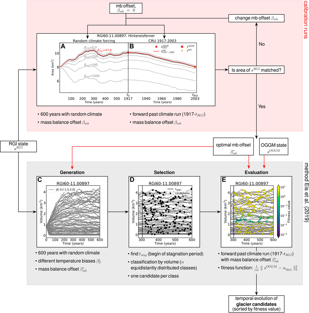
FIGURE 1. Workflow of the calibration runs and the ensemble approach from Eis et al. (2019). (A,B) Calibration runs; the gray lines indicate the iteration procedure and the brown line the result obtained with the optimal mass balance offset ${\beta }_{mb}^{\text{*}}$. (A) The generation of $s_{1917}^{OGGM}$ (marked as red point) using a run forced by random climate with the iteratively chosen mass balance offset ${\beta }_{mb}$. $s_{1917}^{OGGM}$ is then used as starting point of the run in (B). (B) Past climate run with ${\beta }_{mb}$ from $t_0=\mathrm{1,917}$ to the inventory date $t_{RGI}=\mathrm{2,003}$ (for this example). Different ${\beta }_{mb}$ will be tested until the area of the RGI state ($s^{RGI}$, marked as orange square) is matched in $t_{RGI}$ (in this example $t_{RGI}=\mathrm{2,003}$). $s^{OGGM}$ (marked as red square), according to the optimal mass balance offset ${\beta }_{mb}^{\text{*}}$, is the closest to $s^{RGI}$. (C–E) Ensemble approach from Eis et al. (2019). (C) Generation of potential glacier candidates. The gray lines indicate the glacier volume evolution for a set of different random climate scenarios over 600 years each. The temperature biases vary between −1.5 and 3.0 K. (D) Selection of candidates. The black vertical line indicates $t_{stag}$, and the black points show 200 candidates. (E) Glacier candidates colored by their fitness value. Violet marks candidates with a small misfit, whereas yellow marks states that do not meet the acceptance criterion.

As the mass balance offset will be subtracted from the modeled mass balance, the mass balance offset is increased if the area of $s^{OGGM}$ is larger than the area of the RGI state. For this purpose, the lower bound a will be set equal to the midpoint c. Inversely, a smaller mass balance offset ${\beta }_{mb}$ is tested when the area of $s^{OGGM}$ is smaller. Here, the upper bound b is set equal to c. The new midpoint $c=\frac{a+b}{2}$ is calculated, and a new OGGM state is generated with the mass balance offset ${\beta }_{mb}=c$.

This procedure is repeated until the maximum number of iterations $n_{max}=12$ is reached or the area difference falls below the threshold of $1e^{-4}$ km². Thanks to the quick convergence of the bisection method, $n_{max}=12$ is sufficient to determine the mass balance offset with an accuracy of ${\epsilon }_{{\beta }_{mb}}=1$ mm w.e. A continuation of the bisection method would only increase ${\beta }_{mb}$ in the decimals, whereas the area difference would only improve a very little bit further.

The optimal mass balance offset ${\beta }_{mb}^{\text{*}}$, which produced the OGGM state with the smallest area difference to the RGI state, and the corresponding OGGM state $s^{OGGM}$ (marked as red square in Figure 1B) are then used for an initialization with the method from Eis et al. (2019).

Results

We apply our method to all glacier outlines from the RGI (version 6) that can either be linked to mass balance observations provided by the World Glacier Monitoring Service (WGMS, 2017) or to the glacier length records from Leclercq et al. (2014). We exclude all Antarctic and Subantarctic glaciers (RGI region 19), because no CRU data are available for this region. Additionally, we exclude glaciers that are strongly connected to the Greenland ice sheet (connectivity Level 2 in Rastner et al., 2012). Because of the complex dynamical response of water-terminating glaciers, they are excluded as well. We detect them by using the corresponding RGI attribute. This leads to a total sample size of 519 glaciers. For 253 glaciers, there are mass balance time series, and for 317 glaciers, there are length records (51 glaciers have both). The identification of glaciers in the Leclercq dataset in the RGI is done as in Parkes and Goosse (2020). In our study, we use the two suggested types of matches: the positive matches (the (lon,lat) pair from the Leclercq data lies within the RGI outline or within rounding distance to the outline, and the areas in both datasets are similar to each other) and the best effort matches (the glacier cannot be identified uniquely, as, e.g., the (lon,lat) pair is on the border between two glaciers and none or both glaciers satisfy the area criteria). During the calibration runs, two glaciers failed due to processing errors, and thus, we were able to initialize the glacier states in $t_0=1917$ for 517 glaciers. The end of the past climate run $t_e$ is set to the acquisition date of the RGI outline $t_{RGI}$, and thus, it can vary between individual glaciers.

Optimized Mass Balance Offsets

We perform the calibration runs for all tested glaciers as described in Glacier-Specific Calibration of the Mass Balance Model and obtain for each of the glaciers an optimal mass balance offset ${\beta }_{mb}^{\text{*}}$. In Figure 2A, the distribution of the derived mass balance offsets ${\beta }_{mb}^{\text{*}}$ of all glaciers is shown. It is a leptokurtic distribution (positive kurtosis), which is slightly skewed to the right. The values are centered at a mean value of $\mu =5.8\mathrm{ mm w}\mathrm{.e}\mathrm{.}$, and the standard deviation is $\sigma =267.9\mathrm{ mm w}\mathrm{.e}\mathrm{.}$ The mass balance offsets ${\beta }_{mb}^{\text{*}}$ obtained by the calibration runs are of similar magnitude and distribution such as the mass balance offsets obtained by the method from Marzeion et al. (2012).

FIGURE 2

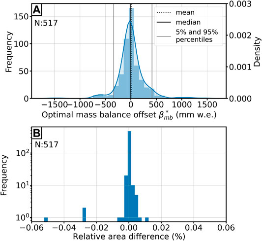
FIGURE 2. (A) Distribution of the derived optimal mass balance offsets ${\beta }_{mb}^{\text{*}}$. Vertical lines indicate the mean (dashed line), median (black line), and the 5 and 95% percentiles (gray lines). The sample size is $n=517$. (B) Histogram of all relative area differences ($\text{\%}$) of the OGGM state $s^{OGGM}$ and RGI state $s^{RGI}$. The sample size is $n=517$. Note that the y-axis is logarithmic.

Figure 2B demonstrates that $s^{OGGM}$ matches the area of $s^{RGI}$ very well in all cases. The mean relative area difference across all glaciers is -0.012%, and also the 5th and 95th percentiles of the relative area error are with values of $Q_{0.05}=-0.064\%$ and $Q_{0.95}=0.089$ very small. The outliers stem from very small glaciers; for example, the largest relative error (−5.2%) occurs for the Northern Schneeferner (Central Europe, Alps), which has a small RGI area of 0.351 km². The absolute area difference to the RGI state is for this glacier −0.02 km². The largest absolute area difference with 2.9 km² occurs for the Breiðamerkurjökull (Iceland, RGI region 06), which had an area of 1,067.7 km² in the year $t_{RGI}=\mathrm{2,000}$.

Reconstructions in the Year 1917

We use the calibration runs to identify optimal mass balance offsets for each of the glaciers and apply the initialization method from Eis et al. (2019) to reconstruct their states in year 1917. The derived mass balance offsets ${\beta }_{mb}^{\text{*}}$ are applied to all model runs during the initialization (the random climate runs and the past climate runs). This ensures that the reconstructed state at the inventory date is in close proximity to the RGI state $s^{RGI}$ and thus allows a comparison with glacier observations. For the reconstruction, we use a fitness function based on geometry differences to the observed glacier state (see Eis et al., 2019, for more details). We here use the OGGM state $s^{OGGM}$ obtained from the calibration runs as the observed glacier state and evaluate the glacier candidate states with the following fitness function:

$J\left(s_{t_0}\right)=\frac{1}{\mathit{ϵ}m}\left({\displaystyle \sum _{i=0}^m{\left({\left(z_{t_{RGI}}^{OGGM}\right)}_i-{\left(z_{t_{RGI}}\right)}_i\right)}^2+{\left({\left(w_{t_{RGI}}^{OGGM}\right)}_i-{\left(w_{t_{RGI}}\right)}_i\right)}^2}\right),(1)$

with the uncertainty $\mathit{ϵ}=125$ and m the total number of grid points of all flow lines of a glacier. The fitness function $J\left(s_{t_0}\right)$ calculates the averaged difference in surface elevation $z_t$ and width $w_t$ between the OGGM state ($s_t^{OGGM}$, obtained from the calibration runs) and the forward modeled glacier states. Eis et al. (2019) showed that a fitness function based on glacier geometry (as used here) leads to the smallest uncertainty of the reconstruction method itself. Taking only limited information into account (e.g., glacier area or length) will increase the uncertainty of the method. Each glacier candidate is evaluated based on the difference to the OGGM state at the inventory date $t_{RGI}$. All states that have a fitness value smaller than 1 are called acceptable states and Eis et al. (2019) suggested the median state (in the following referred to as $s^{med}$) of the 5th percentile of all acceptable states as the best representative of this set. Figure 3 demonstrates the advantages compared to an evaluation based on the RGI state $s^{RGI}$. Indeed, the range of acceptable candidates (with fitness values smaller than one) is similar for both evaluations, but a clear distinction between the best candidates is missing when using $s^{RGI}$. This occurs because the geometry of $s^{RGI}$ is not matched perfectly for any of the tested glacier candidates. As $s^{RGI}$ results from observational data (RGI outline and DEM with different inventory dates) directly, the shape cannot be reproduced exactly by a transient state of the model. The poor distinction between the best candidates would impede the selection of the median state and thus an evaluation based on $s^{RGI}$ could lead to false results. In Optimized Mass Balance Offsets, we could show that the area difference between $s^{RGI}$ and $s^{OGGM}$ is very small for all tested glaciers. In Table 1, we additionally provide the mean values of the relative differences in glacier length and volume. Note that these values are influenced by some single outliers. Nevertheless, $s^{RGI}$ is well represented by $s^{OGGM}$. Figures 3A,C, including Table 2, additionally show the small differences between $s^{RGI}$ and $s^{OGGM}$, using the Hintereisferner as an example.

FIGURE 3

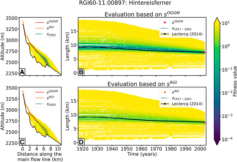
FIGURE 3. Results for the Hintereisferner (Ötztal, Austria). Evaluation of the glacier candidates by fitness function based on geometry differences to (A,B) the OGGM state $s^{OGGM}$ and (C,D) the RGI state $s^{RGI}$. Left: cross-sections along the main flow line in 2003. Black lines indicate the bed rock, red line the OGGM state $s^{OGGM}$, and orange line the RGI state $s^{RGI}$, and the remaining lines indicate the modeled ice surfaces of all candidates, colored by their fitness value. Right: reconstructed glacier length changes (smoothed with 5-year window) from 1917 to 2003. The glacier candidates are colored by their fitness values. The black line with dots shows the glacier length observations from Leclercq et al. (2014). The red square in (B) marks the length of the OGGM state in 2003 and the orange square in (C) the length of the RGI state in 2003.

TABLE 1

TABLE 1. Glacier length, area, and volume of the median state in 1917 and 2003 of Hintereisferner (Ötztal, Austria).

TABLE 2

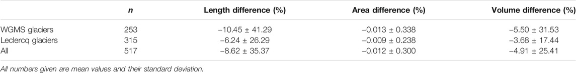
TABLE 2. Relative differences (in $\text{\%}$) in glacier length, area, and volume between the RGI state $s^{RGI}$ and the OGGM state $s^{OGGM}$ (obtained from the calibration runs).

Validation with Glacier Observations

The uncertainty analysis in Eis et al. (2019) showed that the uncertainty of our method reduces quickly over time. As a result, a meaningful validation of the method, which also covers the time period with the largest uncertainties, should ideally be performed with observations starting before or at the beginning of the initialization year (at the beginning of the 20th century). Remote-sensing techniques are available for a relatively short time period and are consequently not of sufficient length for validation purposes. More suitable are direct observations of glacier mass change, which start to increase in number from the year 1950 onward. Here, we use glacier-wide mass balance observations provided by the World Glacier Monitoring Service (WGMS, 2018). The Fluctuations of Glaciers (FoG) database contains annual mass balance values for several hundreds of glaciers worldwide, but only 40 reference glaciers have record longer than 30 years. Thus, we additionally include glacier length change observations to our validation, as they date back furthest in time. They are usually obtained through annual measurements of the terminus position, but they can also be reconstructed from geomorphologic landforms (e.g., moraines) and biological evidence (e.g., overridden trees and lichens) (e.g., Bushueva et al., 2016) or from historical paintings, photos, and early maps (e.g., Nussbaumer and Zumbühl, 2012). The dataset of Leclercq et al. (2014) includes long-term glacier length records that start no later than 1950 and span at least 40 years. The temporal frequency and spatial accuracy of the dataset increase rapidly from 1900 onward (Leclercq et al., 2014).

As the initialization method results in nonunique solutions, we use the median state $s^{med}$ of the 5th percentile (the 5% best glacier candidates, using the fitness function from Eq. 1) as basis for the validation. How certain this representative is depends strongly on the nonuniqueness of the solution. Eis et al. (2019) presented a measure which shows how well a glacier can be reconstructed based on the range of nonunique solutions and called this the “reconstructability” of a glacier. The reconstructability is low (close to zero) if the majority of all glacier candidates have a small fitness value. The reconstructability is high (close to one) if an almost unique solution can be found. Figure 4 shows the distribution of the reconstructability values for all glaciers included in this study. Almost all tested glaciers have a high reconstructability, which means that the range of possible solutions is really narrow. Subsequently, the median state is a particularly good representative for these cases.

FIGURE 4

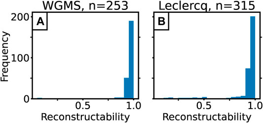
FIGURE 4. Distribution of the reconstructability values of all glaciers used in this study. (A) The values from the glaciers used for the validation with the WGMS dataset and (B) from the glaciers used for the validation with the Leclercq et al. (2014) dataset.

The median state is then used as initial condition for a forward run, using the past climate from 1917 until the RGI date $t_{RGI}$. From this temporal evolution, we select the years with measurements and gain a total set of 5,325 pairs of annual modeled and measured glacier-wide mass balances and a set of 10,420 pairs of annual modeled and observed glacier length changes.

The validation is performed based on five different error criteria: the model error, the mean bias error (MBE), the mean absolute error (MAE), the root mean square error (RMSE), and the correlation r. A summary of the performance can be found in Table 3. When referring in the following to one of the mass balance errors, a subscripted $mb$ will be added (e.g., RMSE_mb). Accordingly, we will add a subscripted L when referring to one of the glacier length errors (e.g., RMSE_L).

TABLE 3

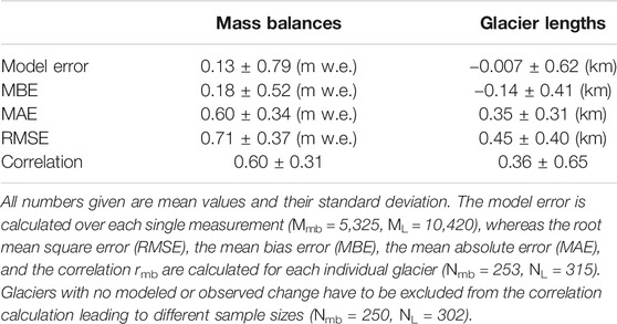
TABLE 3. Summary of the comparisons of modeled and measured mass balances and glacier length records.

Mass Balance Validation

Before presenting the mass balance validation in detail, we show the results of three different example glaciers and the corresponding observations from WGMS (2018) in Figure 5. Figure 5A shows an example with an almost perfect match to the observation, whereas the other two figures show two examples with a bad performance. In the example in Figure 5B, mass balances are well matched until 1975, but afterwards the modeled mass balances are high compared to the observation. The glacier shown in Figure 5C fits the observation on average, but the modeled amplitude is far too small. Here, the smaller variability in the modeled mass balances originates from the calibrated precipitation correction factor $p_f$, which is set to a global value of 2.5. The influence of the precipitation correction factor on the variability of the modeled mass balance is shown in, e.g., Marzeion et al. (2012). The underestimation of the variability in the OGGM is quantified with approx. 10% (see Maussion et al., 2019; Appendix A). The results of each individual glacier are provided in the supplement.

FIGURE 5

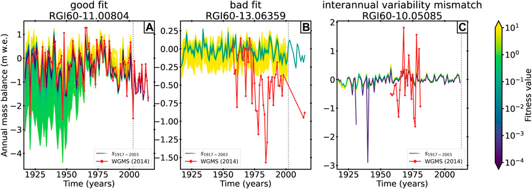
FIGURE 5. Reconstructed annual mass balances from 1917 onward of three example glaciers. Figures from all glaciers used in this study can be found in the supplement. (A) RGI60–11.00804, region 11 (Central Europe), (B) RGI60–13.06359, region 13 (Central Asia), and (C) RGI60–10.05085, region 10 (North Asia). The lines are colored by their fitness values. The red line with dots indicates the observed annual mass balances from WGMS (2018). The dots mark years with observations. The vertical dashed line marks $t_{RGI}$, from which onward only the median state is modeled forward in case observations after $t_{RGI}$ are available.

Mass Balance Model Error

The mass balance model error is calculated for each of the 5,325 pairs of annual modeled and measured mass balances. For each pair, the measured mass balance is subtracted from the modeled mass balance at the same year.

Table 3 shows that the mean over all mass balance model errors is with a value of −0.13 m w.e. close to zero, and also, the standard deviation (0.79 m w.e.) indicates a good fit between modeled and observed mass balances. Figure 6 shows a binned scatter plot of the mass balance model errors over time and thus provides information about their temporal distribution. In addition, the temporal distribution of the mass balance measurements (Figure 6A) and the distribution of the mass balance model errors (Figure 6C) are shown. With an increasing number of measurements since 1960, the counts raise, especially in the middle range between −1 and 1 m w. e. Most values are in close proximity to zero, but single errors reach values up to $\pm$ 4 m w.e. The mass balance model errors are normally distributed (see Figure 6). The correlation between the model error and the time is with $r=0.008$ close to zero which indicates that there is no trend.

FIGURE 6

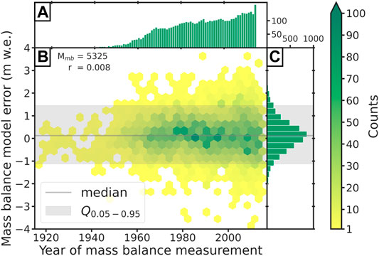
FIGURE 6. Mass balance model error. (A) Histogram of mass balance measurements per year. (B) Binned scatter plot of model errors over time. The colors indicate the counts of errors in each bin. The numbers in the upper left corner indicate the total number of errors and the correlation with the time. (C) Distribution of the modeled mass balance errors.

Mean Bias Error (MBE_mb)

The mean bias error (also referred as bias, e.g., in Marzeion et al. (2012)) is calculated for each of the 253 glaciers with mass balance measurements:

${\text{MBE}}_{\text{mb}}=\frac{1}{\text{n}}{\displaystyle \sum _{1=1}^n\left(\text{B}{\left(\text{i}\right)}_{\text{modeled}}-\text{B}{\left(\text{i}\right)}_{\text{measured}}\right)},(2)$

where n is the total number of years with mass balance measurements for the specific glacier. Thus, the MBE_mb provides information about the performance of individual glaciers. Figure 7A shows that the MBE_mb is small for the majority of the glaciers. This is also reflected by the small mean (0.18 m w.e.) and median (0.14 m w.e.) values. Nevertheless, a few outliers range up to 2 m w.e. The distribution is slightly positive skewed, indicating that the mass balance is marginally overestimated by the model on average.

FIGURE 7

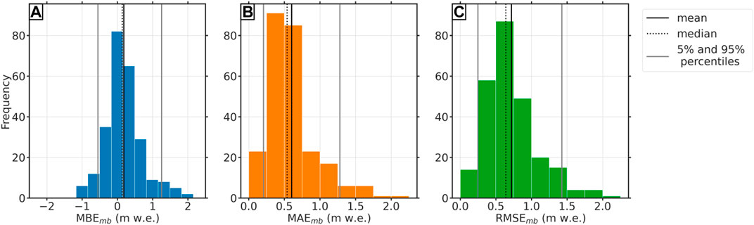
FIGURE 7. Histogram of (A) MBE_mb (mm w. e.), (B) MAE^mb (mm w. e.), and (C) RMSE_mb (mm w. e.). Each histogram has a sample size of N_mb = 253.

Mean Absolute Error (MAE_mb) and RMSE_mb

The root mean square error (RMSE_mb; Eq. 3) and the mean absolute error (MAE_mb; see Eq. 4), calculated for each glacier as well, do not consider the direction of the error. Thus, they provide more information about the magnitude of the errors than the MBE_mb:

${\text{RMSE}}_{\text{mb}}=\sqrt{\frac{1}{\text{n}}{\displaystyle \sum _{i=1}^n{\left(\text{B}{\left(\text{i}\right)}_{\text{modeled}}-\text{B}{\left(\text{i}\right)}_{\text{measured}}\right)}^2}},(3)$

${\text{MAE}}_{\text{mb}}=\frac{1}{\text{n}}{\displaystyle \sum _{i=1}^n\left(\text{B}{\left(\text{i}\right)}_{\text{modeled}}-\text{B}{\left(\text{i}\right)}_{\text{measured}}\right)}.(4)$

The RMSE_mb gives a relatively strong weight to large errors since the errors are squared before they are averaged and thus the values are larger than the ones of the MAE_mb (see Figures 7B,C; Table 3). Their distributions are quite similar to each other, and also, their mean values are in close proximity to each other (0.60 m w.e. for MAE_mb and 0.71 m w.e. for RMSE_mb). Also, their standard deviation does not differ significantly. Both measures show that the magnitude of the error is small for most glaciers. Even the few outliers fit the observation with an RMSE of about 2 m w.e. well.

Correlation r_mb

Beside the different types of errors, we calculate the correlation between the modeled and measured mass balances over all glaciers. The negatively skewed distribution of the correlation coefficients in Figure 8A shows that for most glaciers, the correlation is high. Nevertheless, for some single glaciers, the modeled mass balances do not correlate with the measurements. Some glaciers even have a negative correlation, which distinctly influences the mean value across all glaciers. Figure 8B shows that there is a relation between the correlation coefficients $r_{mb}$ and the number of mass balance measurements per glacier. All low and negative correlation coefficients result only from glaciers with less than 30 years of mass balance measurements. In addition, low and negative correlation values only occur when the correlation is not significant (at the 5% level). However, Figures 8A,B also shows that the correlation is high for the majority of glaciers, even if only the ones with less than 30 years of mass balance measurements are considered. Nevertheless, it becomes clear that the mean value (0.60) over all glaciers is largely influenced by these outliers. In order to reduce this effect, we calculated an average value weighted by the number of mass balance measurements per glacier and we obtain a weighted mean correlation of 0.67 across all glaciers. This shows that the modeled mass balances are in good agreement with the observations.

FIGURE 8

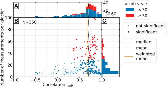
FIGURE 8. Correlation coefficients in relation to number of mass balance measurements per glacier. Red dots or bars mark glaciers with more than 30 years of mass balance measurements and blue marks glaciers with less than 30 years. (A) Histogram of the correlation coefficients of all glaciers. (B) Scatter plot of the correlation against the number of mass balance measurements. A large dot indicates a correlation value that is significant at the 5% level and a small dot a not significant value. The horizontal, black line indicates the mean value over all glaciers, the orange line the average correlation weighted number of mass balance measurements per glacier, and the dotted, black line the median value. (C) Histogram of number of mass balance measurement per glacier. Note that the sample size is N = 250, because the WGMS dataset contains three glaciers with constant mass balance series, and due to the zero variance, it is consequently not possible to calculate the correlation.

Glacier Length Validation

In addition to the validation with the mass balance time series from the WGMS dataset, in this section, we compare modeled and observed glacier length changes. As before, we will use the modeled glacier length from the median state of the reconstruction. A clear advantage of glacier length fluctuations is the better temporal coverage compared to the mass balance observations. Some of the length observations even start prior to 1850. Eis et al. (2019) showed that largest uncertainties of the reconstruction method occur at the beginning of the initialization (in this study 1917) and consequently a validation with many early observations is particularly helpful. We transform the glacier length changes from Leclercq et al. (2014) into respective glacier length values. To this end, we first determine all glacier length changes relative to the RGI inventory date $t_{RGI}$. When no observation is available in $t_{RGI}$, we interpolate the length change for this year. In case the year of the last length change observation is before $t_{RGI}$, we use the last observation year instead. Finally, we reconstruct the observed glacier length time series with the help of the median state and add their glacier length at $t_{RGI}$ or at the last observation year, such that observed glacier length and the reconstructed glacier length are identical at this date.

In some cases, $t_{RGI}$ is long before the year of the last length change observation. In order to make use of these observations, we additionally run the median state from $t_{RGI}$ to the last observation year using the same past climate run as during the initialization procedure. In total, we gain a set of 10,420 pairs of modeled and observed glacier lengths since 1917. In Figure 9, we show the results of three different example glaciers and the corresponding observed glacier length from Leclercq et al. (2014). Figure 9A shows an example with an almost perfect match to the observation, whereas the other two figures show two examples with a bad performance. The example in Figure 9B is the glacier with largest MBE_L value. The glacier shown in Figure 9C has a negative correlation value of −0.77, as the best glacier candidate shows a clear glacier advance over the whole time period, whereas the observation indicates a clear glacier retreat. More examples are provided in the supplement.

FIGURE 9

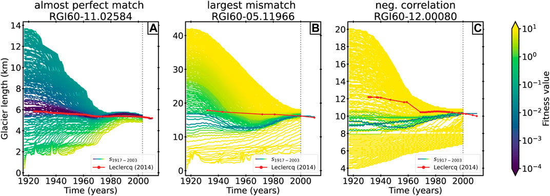
FIGURE 9. Reconstructed glacier lengths from 1917 onward of three example glaciers. Figures from all glaciers used in this study can be found in the supplement. (A) RGI60–11.02584, region 11 (Central Europe), (B) RGI60–05.11966, region 05 (Greenland), and (C) RGI60–11.00090, region 12 (Caucasus and Middle East). The lines are colored by their fitness values. The red line with dots indicates the observed glacier length from Leclercq et al. (2014). The dots mark years with observations. The vertical dashed line marks $t_{RGI}$, from which onward only the median state is modeled forward in case observations after $t_{RGI}$ are available.

Table 3 shows a summary of the performance of all tested glaciers described by the length error, the mean bias error (MBE_L), the mean absolute error (MAE_L), the root mean square error (RMSE_L), and the correlation r_L.

Length Error

Similar to the mass balance model error in Mass Balance Validation, we calculate the length error for each of the 10,420 pairs of modeled and observed glacier length. In opposition to the other errors (MBE_L, MAE_L, RMSE_L, and r_L), the length error is not calculated per glacier, but every data point contributes in equal proportions.

Figure 10B shows the distribution of the length errors over time. Most of the values range between ±1 km (see also Figure 10C), and also the small mean value over all length errors of −0.007 km indicates a good agreement with the observations. Nevertheless, a lot of outliers range up to ±3 km and very few values have a length error about ∼6 km (see Figure 10B). This also influences the standard deviation which has a value of 0.62 km. A correlation of the length errors with time is not identifiable (r = −0.118), and the data coverage is good over the whole time period (see Figure 10A).

FIGURE 10

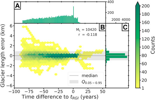
FIGURE 10. Glacier length error. (A) Histogram of glacier length observations per year. Note that the x-axis is displayed in time difference to $t_{R}GI$. Thus, all glacier length errors in $t_{RGI}$ (x = 0) are zero. (B) Binned scatter plot of model errors over time. The colors indicate the counts of errors in each bin. The numbers in the upper left corner indicate the total number of model errors and the correlation with the time. (C) Distribution of the glacier length errors.

Mean Bias Error (${\text{MBE}}_{\text{L}}$)

The mean bias error (${\text{MBE}}_{\text{L}}$) is calculated for each of the 315 glaciers with length observations. The ${\text{MBE}}_{\text{L}}$ provides information about how well the glacier length of individual glaciers is reproduced. The mean value over all MBE_L is with −0.14 km small, and also the standard deviation with a value of 0.41 km indicates a good fit. This can also be seen in the histogram in Figure 11A which shows clearly that the majority of the values range between ±0.5 km, but larger errors are possible as well. The 5th and 95th percentiles range from −0.89 to 0.4 km, whereas the largest error (−1.7 km) occurs for a glacier located in southeast Greenland (RGI60-05.11966). The distribution of all MBE_L values is slightly skewed left, indicating that the reconstruction method tends to underestimate the glacier lengths. As a large misfit between modeled and observed glaciers can also stem from a large glacier, we calculated additionally to the absolute error value per glacier the mean bias errors relative to the observed glacier length at the RGI date (see Figure 11D for more details). The histogram of the MBE_L (in %) clearly shows that a majority of values range between −12.5 and 12.5%, which is also reflected by the values of the 5th and 95th percentiles which ranges from −18 to 13%. These small values support the assumptions of a very good agreement between the observed and modeled glacier lengths.

FIGURE 11

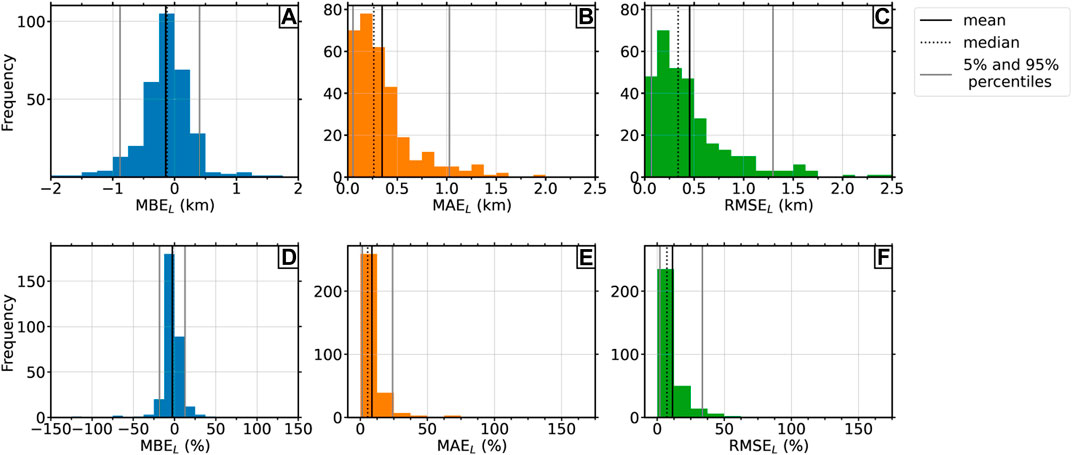
FIGURE 11. Histograms of (A) the mean bias errors (km), (B) the mean absolute errors (km), (C) the root mean square error (km), (D) the mean bias errors ($\text{\%}$), (E) the mean absolute errors ($\text{\%}$), and (F) the root mean square error ($\text{\%}$). Each histogram has a sample size of N = 315. The horizontal, black lines represent the mean value, the dashed lines the median, and the gray line the corresponding 5th and 95th percentiles.

Mean Absolute Error (${\text{MAE}}_{\text{L}}$) and RMSE_L

The MAE_L and RMSE_L provide more insights about the magnitude of the errors than the MBE_L, as negative and positive values cannot be compensated. Thus, the mean overall MAE_L and RMSE_L values are with values of 0–35 km (for MAE_L) and 0.45 km (for RMSE_L) noticeable higher than the ones from the length errors or the MBE_L (see Table 3). The standard deviations are slightly smaller (0.31 km for MAE_L and 0.4 km for RMSE_L), but this can be explained due to the reduced range of possible values (only positive). The histograms in Figure 11 show that the majority of the errors is small. Considering, e.g., the MAE_L, then half of the errors are smaller than 0.26 km, which indicates a very good fit between the modeled and observed glacier lengths. Outliers range again up to ∼2 km for MAE_L and up to ∼2.4 km for RMSE_L, but they occur very rarely. In general, the RMSE_L errors are a little bit higher than those of the MAE_L which is due to the relatively strong weight to large errors during the RMSE calculation. When considering the errors relative to the glacier lengths, the majority of the MAE_L (in %) and RMSE_L (in %) values are smaller than 25%. The 95th percentiles are located in both cases under 50% (24% for the MAE_L and 34% for the RMSE_L), which confirm the good fit.

Correlation r_L

The results from the correlation analysis of the modeled and observed glacier lengths, calculated for each glacier individually, do not indicate a good agreement for all tested glaciers. The distribution of the individual correlation coefficients for each glacier is slightly bimodal (see Figure 12A). Most correlation values range from 0.7 to 1, but 87 out of 302 glaciers have a negative correlation (some of them close to −1). In contrast to the correlation analysis from the mass balances (see Figure 8B), not all negative correlation values can be explained by a low number of observations or because the correlation is not significant at the 5% level. Figure 12B shows that 12 glaciers with more than 30 length observations have a negative correlation, and four of them are even in close proximity to −1.

FIGURE 12

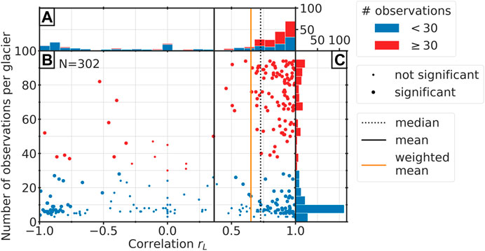
FIGURE 12. Correlation coefficients in relation to total number of glacier length observations per glacier. Red dots or bars mark glaciers with more than 30 years of measurements and blue marks glaciers with less than 30 years. (A) Histogram of the correlation coefficients of all glaciers. (B) Scatter plot of the correlation against the number of glacier length observation. Horizontal, black line indicates the mean value over all glaciers, the orange line the average correlation weighted by the number of observations per glacier, and the dotted, black line the median value. (C) Histogram of the number of glacier length observations per glacier. Note that the sample size is N = 302, because for 13 glaciers, the modeled glacier length is constant, and due to the zero variance, it is consequently not possible to calculate the correlation.

An example of one of these outliers can be found in Figure 9C. The reconstructed state in 1917 is far too small, requiring that the glacier needs to advance continuously to reach the present-day state. In contrast to that, the observed glacier retreated over the entire period, which leads to a strong negative correlation. In the figure, one can see that glacier candidates exist which would have reflected the observation very well. However, these candidates have high fitness values, which could, e.g., stem from a bad representation of the OGGM state or from a poorly chosen parameter setup of the mass balance model or dynamical model for individual glaciers.

Nevertheless, the histogram and the scatter plot in Figures 2B, 12A show that a majority of the glaciers with negative correlation values can be attributed to a low number of length observations. The negative correlation values largely influence the mean value (0.36), for what reason the mean weighted over the number of observations per glacier is with a value of 0.65 more representative. This is also underlined by the even higher median value (0.73).

Discussion and Conclusion

This study extends Eis et al. (2019) with the addition of mass balance calibration runs, to adapt the method to real-world use cases. After the standard calibration of the mass balance model, we additionally perform a glacier-specific calibration of the mass balance offset ${\beta }_{mb}$, which is iteratively calibrated, such that the glacier state at the inventory date is in close proximity to the observation. The obtained mass balance offset ${\beta }_{mb}$ is then applied to all (past and random climate) forward runs during the initialization procedure. We apply the initialization method to 517 glaciers, for which either mass balance measurements or glacier length records are available.

Water-terminating glaciers are excluded from this study, because a dynamical forward model for tide-water glaciers would be required, which is still under development and validation. For their identification, the attribute from the RGI database is used, but this characteristic only refers to the inventory date $t_{RGI}$. Besides this, there is no other possibility in the OGGM to identify water-terminating glaciers. This would be necessary to detect glaciers which were water-terminating at some point in the past, but they are not anymore at the inventory date $t_{RGI}$. Such glaciers are treated as non-water-terminating glaciers, which is a potential source of large length errors, as, e.g., frontal ablation is not considered.

We validate our initialization method by comparing modeled glacier changes to mass balance observations (WGMS, 2018) and to length records (Leclercq et al., 2014). For this purpose, different types of errors (model error, mean bias error, mean absolute error, root mean square error, and correlation) are taken into account. As the initialization can result in nonunique solutions, we use the median state of the 5th percentile for the validation. This is the best representative for the possibly large set of acceptable glacier states (see Eis et al., 2019, for more details), which is additionally justified by the high reconstructability values for glaciers in this study. Unfortunately, this also means that glaciers with a low reconstructability are underrepresented in our study. Eis et al. (2019) showed a negative correlation between the reconstructability of a glacier and its slope. We speculate that this could be one reason for the high reconstructability values in our study, as observations are biased towards the accessibility of a glacier. Another reason could be the positive correlation between the response time of a glacier and its reconstructablity. The considered time interval in this study from 1917 to the present day does not seem to exceed the response time by a large amount for the majority of the investigated glaciers.

Altogether, the validation shows a good agreement between the modeled glacier states and the observations. Considering the mass balance observations, a mean model error (calculated over each pair of modeled and measured mass balances) of 0.13 $\pm$ 0.79 m w.e. is achieved. We find that the correlation between the modeled and the measured time series is influenced by the number of mass balance measurements. Negative and low correlation coefficients are exclusively produced when the number of mass balance observations for this glacier is low (less than 30 years). Eis et al. (2019) showed that the uncertainties that stem from the initialization method itself are largest during the first years after the initialization. Unfortunately, most of the mass balance observations were made after 1960. Prior mass balance measurements exist for very few individual glaciers only. For this purpose, we add the comparison with glacier length records from Leclercq et al. (2014) to our validation, which have a better temporal coverage at the beginning of our initialization in 1917. In addition, the validation based on the length changes represents an out-of-sample, as this dataset is not used for the calibration of the OGGM (in contrast to the mass balance data). Although 51 glaciers have both kinds of observations, a t-test showed that the difference in the statistics is not significant when excluding these 51 glaciers. Considering the glacier length, the mean model error has a value of 0.14 $\pm$ 0.41 km, which emphasizes the good agreement with the observations. The mean correlation value, with 0.36 $\pm$ 0.65, is significantly smaller than the value concerning the mass balances, but again, this is mainly influenced by the many glaciers with few observations. For a better interpretation of these values, we also need to consider the uncertainties of the observations. Zemp et al. (2013) provided an error estimation for the random error from the glaciological mass balance measurements (0.34 m w.e.). To allow a comparison between the calculated model error of the initialization method and the error of the mass balance measurements, we need to calculate the mean of the absolute values of the mass balance model errors. With a value of 0.59 m w.e., it is about twice that of the random error from the glaciological mass balance measurements. Leclercq et al. (2014) provided the information about the data accuracy for each individual data point (depending on the method used for the data acquisition). 97% of the data points used in our study can be assigned to Category 1 (direct measurements) and these measurements typically have a spatial uncertainty of less than 50 m and a time accuracy within 1 year (Leclercq et al., 2014). Compared to the obtained length errors of the initialization method, the error of the lengths observations seems to be negligibly small. Most data points of the remaining 3% are assigned either to Category 2 (historical sources), with a typical uncertainty range of 100–200 m, or to the fifth category, for which the method of measurement is unknown and consequently the accuracy is unknown as well. In addition to the accuracy of the observations, other factors that could influence our validation need to be considered as well. Unfortunately, this is difficult, as they cannot be quantified. Larger uncertainties could, e.g., be produced by a wrong linking between glacier IDs from different datasets. This especially concerns the links between the Leclercq et al. (2014) dataset and the Randolph Glacier Inventory. For linking, we use the method described in Parkes and Goosse (2020), resulting in two classes of matches: positive matches and “best-effort”-matches. Especially for the second class, a false linking cannot be excluded. Another uncertainty could come from false outlines provided by the RGI. These occur due to uncertainties in the topography, unavailable data or because of human decisions (Maussion et al., 2019). False outlines can lead to false centerlines and consequently to errors in the present-day geometry. This results not only in errors in the length calculations, but also in a false RGI state on which the reconstruction is based. Besides the correct representation of the present-day state, the reconstruction method also relies on the assumption of well-known climate conditions. Thus, errors in the used climate data lead to errors in the reconstructed glacier states. Furthermore, modeled and observed length changes can differ in special cases, due to separation of glacier entities in the observation period. As a result, a jump in the observed glacier lengths occurs. At the current time, the model is not yet able to reproduce these jumps. This would require a merging of neighboring glaciers and is already under development. However, the merging method is not yet fully automatized.

Regardless of all these different sources of uncertainty, we can summarize that both datasets, the mass balance observations from WGMS (2018) and the glacier length records from Leclercq et al. (2014), are well matched by the modeled glacier states and thus the initialization method from Eis et al. (2019) is verified for the considered time period.

Applications to longer time scales, e.g., over the last centuries/millennia, would in theory be possible under the condition that the climate is well known. However, the reconstructablity value decreases in time and will thus be a limitation factor for this type of application. Taking into account more large-scale observational data (e.g., multitemporal outlines) could improve the reconstructability further and thus would allow a reconstruction further back in time.

Future work will include a global application, which would be the first global glacier reconstruction using a flow-line model. However, a global run would have a very high computational cost, meaning it will likely take multiple months on our small cluster. Computational costs could potentially be reduced by decreasing the model resolution or the number of the glacier candidates. Additional challenges of global reconstructions originate from the poor representation of glacier complexes and ice caps in flow-line models, which stem from their nontrivial geometries (Maussion et al., 2019). Furthermore, the mentioned problems regarding water-terminating glaciers need to be solved beforehand. Such a global reconstruction would also neglect disappeared glaciers, which are uncharted today (Parkes and Marzeion, 2018). The missing but mandatory present-day outlines make it impossible to reconstruct them, and only multitemporal outlines on a large scale could provide a remedy.

Furthermore, a similar approach to the calibration runs could be used in order to optimize other fundamental dynamical parameters in the OGGM, to improve the behavior of the dynamical model in general. For this purpose, it would be sufficient to consider a much shorter time period than in this study (as it was done, e.g., in Zekollari et al., 2019). The sliding parameter and creep parameter, which in the OGGM by default are not glacier-specific, are, e.g., potential parameters for such an approach. Obviously, also other criteria than a match in present-day area could be taken into account (e.g., glacier length, mean ice thickness, and surface elevation at the head of the glacier). Such an approach could not only further improve the reconstruction of glaciers, but also future projections.

Hardware Requirements and Performance

For this study, we used a small cluster comprising two nodes with two 14-core CPUs each, resulting in 112 parallel threads (two threads per core). As the mass balance offset calibration converges within 12 iterations, running the calibration runs is cheap. The application of the initialization method from (Eis et al., 2019) is more expensive, as hundreds of dynamical model runs need to be performed and the dynamical runs are the most expensive computations in the OGGM. The size of the glacier and the required time stepping to ensure a numerical stability (adaptive time step following the CFL criterion) strongly influence the required computation time. The computation time needed to apply the initialization procedure to one glacier varies from glacier to glacier. In total, initializing the 517 glaciers in 1917 takes approximately 24 h on our small cluster. This implies that substantial computing resources will be needed in order to apply our method to, e.g., initialize a global model run.

Code Availability

The OGGM software together with the initialization method is coded in the Python language and licensed under BSD-3-Clause License. The latest version of the OGGM code is available on GitHub (https://github.com/OGGM/oggm), the documentation is hosted on ReadTheDocs (http://oggm.readthedocs.io), and the project webpage for communication and dissemination can be found at http://oggm.org. OGGM version used in this study is v1.2. The code for the initialization module is available on GitHub (https://github.com/OGGM/initialization).

Data Availability Statement

All data and code used in this study can be found on a public repository at https://github.com/OGGM/initialization, and the version used for this paper is archived with a DOI at http://doi.org/10.5281/zenodo.4625362. The OGGM version used for this study is 1.2, archived at http://doi.org/10.5281/zenodo.3597756.

Author Contributions

JE is the main developer of the initialization module and wrote most of the paper. LL supported the development of this study and worked on methodological concepts and testing. BM and FM are the initiators of the OGGM project and helped to conceive this study. FM is the main OGGM developer.

Funding

BM and JE were supported by the German Research Foundation, grants MA 6966/1-1 and MA 6966/1-2. LL was supported by the German Research Foundation, grant FO 1269/1-1. FM acknowledges support from the Austrian Science Fund (FWF) Grant P30256-NBL.

Conflict of Interest

The authors declare that the research was conducted in the absence of any commercial or financial relationships that could be construed as a potential conflict of interest.

Supplementary Material

The Supplementary Material for this article can be found online at: https://www.frontiersin.org/articles/10.3389/feart.2021.595755/full#supplementary-material.

References

Bamber, J., Westaway, R. M., Marzeion, B., and Wouters, B. (2018). The land ice contribution to sea level during the satellite era. Environ. Res. Lett. 13 (6). doi:10.1088/1748-9326/aac2f0

CrossRef Full Text | Google Scholar

Biemans, H., Siderius, C., Lutz, A., Nepal, S., Ahmad, B., Hassan, T., et al. (2019). Importance of snow and glacier meltwater for agriculture on the indo-gangetic plain. Nat. Sustainability 2, 594–601. doi:10.1038/s41893-019-0305-3

CrossRef Full Text | Google Scholar

Bushueva, I., Solomina, O., and Volodicheva, N. A. (2016). Fluctuations of terskol glacier, northern caucasus, Russia. Earth’s Cryosphere 20, 95–104. doi:10.21782/KZ1560-7496-2016-3(95-104

CrossRef Full Text | Google Scholar

Church, J., Clark, P., Cazenave, A., Gregory, J., Jevrejeva, S., Levermann, A., et al. (2013). Sea level change, Cambridge, United Kingdom and New York, NY, USA: Cambridge University Press, 13. 1137–1216. doi:10.1017/CBO9781107415324.026

CrossRef Full Text

Eis, J., Maussion, F., and Marzeion, B. (2019). Initialization of a global glacier model based on present-day glacier geometry and past climate information: an ensemble approach. The Cryosphere 13, 3317–3335. doi:10.5194/tc-13-3317-2019

CrossRef Full Text | Google Scholar

Farinotti, D., Huss, M., Bauder, A., Funk, M., and Truffer, M. (2009). A method to estimate the ice volume and ice-thickness distribution of alpine glaciers. J. Glaciology 55, 422–430. doi:10.3189/002214309788816759

CrossRef Full Text | Google Scholar

Farinotti, D., Huss, M., Fürst, J. J., Landmann, J., Machguth, H., Maussion, F., et al. (2019). A consensus estimate for the ice thickness distribution of all glaciers on earth. Nat. Geosci. 12, 168–173. doi:10.1038/s41561-019-0300-3

CrossRef Full Text | Google Scholar

Gardner, A. S., Moholdt, G., Cogley, J. G., Wouters, B., Arendt, A. A., Wahr, J., et al. (2013). A reconciled estimate of glacier contributions to sea level rise: 2003 to 2009. Science 340, 852–857. doi:10.1126/science.1234532

PubMed Abstract | CrossRef Full Text | Google Scholar

Giesen, R. H., and Oerlemans, J. (2012). Calibration of a surface mass balance model for global-scale applications. The Cryosphere 6, 1463–1481. doi:10.5194/tc-6-1463-2012

CrossRef Full Text | Google Scholar

Giesen, R. H., and Oerlemans, J. (2013). Climate-model induced differences in the 21st century global and regional glacier contributions to sea-level rise. Clim. Dyn. 41, 3283–3300. doi:10.1007/s00382-013-1743-7

CrossRef Full Text | Google Scholar

Gregory, J. M., White, N. J., Church, J. A., Bierkens, M. F. P., Box, J. E., van den Broeke, M. R., et al. (2013). Twentieth-century global-mean sea level rise: is the whole greater than the sum of the parts?. J. Clim. 26, 4476–4499. doi:10.1175/JCLI-D-12-00319.1

CrossRef Full Text | Google Scholar

Harris, I. C., Jones, P. D., Osborn, T., and Lister, D. (2014). Updated hight-resolution grids of montly climatic observations- the cru ts3.10 dataset. Int. J. Climatology 34, 623–642. doi:10.1002/joc.3771

CrossRef Full Text | Google Scholar

Huss, M., and Hock, R. (2015). A new model for global glacier change and sea-level rise. Front. Earth Sci. 3, 54. doi:10.3389/feart.2015.00054

CrossRef Full Text | Google Scholar

Hutter, K. (1981). The effect of longitudinal strain on the shear stress of an ice sheet: in defence of using streched coordinates. J. Glaciol. 27, 39–56. doi:10.3189/S0022143000011217

CrossRef Full Text | Google Scholar

Hutter, K. (1983). Theoretical glaciology: material science of ice and the mechanics of glaciers and ice sheets. Dordrecht: D. Reidel Publishing Company.

Immerzeel, W. W., Lutz, A. F., Andrade, M., Bahl, A., Biemans, H., Bolch, T., et al. (2020). Importance and vulnerability of the world’s water towers. Nature 577, 364–369. doi:10.1038/s41586-019-1822-y

PubMed Abstract | CrossRef Full Text | Google Scholar

Jacob, T., Wahr, J., Pfeffer, W. T., and Swenson, S. (2012). Recent contributions of glaciers and ice caps to sea level rise. Nature 482, 514–518. doi:10.1038/nature10847

PubMed Abstract | CrossRef Full Text | Google Scholar

Kääb, A., Reynolds, J. M., and Haeberli, W. (2005). glacier and permafrost hazards in high mountains. Dordrecht, Netherlands: Springer Netherlands, 225–234. doi:10.1007/1-4020-3508-X˙23

CrossRef Full Text

Kaser, G., Grosshauser, M., and Marzeion, B. (2010). Contribution potential of glaciers to water availability in different climate regimes. Proc. Natl. Acad. Sci. USA 107, 20223–20227. doi:10.1073/pnas.1008162107

PubMed Abstract | CrossRef Full Text | Google Scholar

Kienholz, C., Rich, J. L., Arendt, A. A., and Hock, R. (2014). A new method for deriving glacier centerlines applied to glaciers in Alaska and northwest Canada. The Cryosphere 8, 503–519. doi:10.5194/tc-8-503-2014

CrossRef Full Text | Google Scholar

Leclercq, P. W., Oerlemans, J., Basagic, H. J., Bushueva, I., Cook, A. J., and Le Bris, R. (2014). A data set of worldwide glacier length fluctuations. The Cryosphere 8, 659–672. doi:10.5194/tc-8-659-2014

CrossRef Full Text | Google Scholar

Marzeion, B., Cogley, J. G., Richter, K., and Parkes, D. (2014). Attribution of global glacier mass loss to anthropogenic and natural causes. Science 345, 919–921. doi:10.1126/science.1254702

PubMed Abstract | CrossRef Full Text | Google Scholar

Marzeion, B., Hock, R., Anderson, B., Bliss, A., Champollion, N., Fujita, K., et al. (2020). Partitioning the uncertainty of ensemble projections of global glacier mass change. Earth’s Future 8, e2019EF001470. doi:10.1029/2019EF001470

CrossRef Full Text | Google Scholar

Marzeion, B., Jarosch, A. H., and Hofer, M. (2012). Past and future sea-level change from the surface mass balance of glaciers. The Cryosphere 6, 1295–1322. doi:10.5194/tc-6-1295-2012

CrossRef Full Text | Google Scholar

Marzeion, B., Kaser, G., Maussion, F., and Champollion, N. (2018). Limited influence of climate change mitigation on short-term glacier mass loss. Nat. Clim. Change 8, 305–308. doi:10.1038/s41558-018-0093-1

CrossRef Full Text | Google Scholar

Marzeion, B., Leclercq, P. W., Cogley, J. G., and Jarosch, A. H. (2015). Brief communication: global reconstructions of glacier mass change during the 20th century are consistent. The Cryosphere 9, 2399–2404. doi:10.5194/tc-9-2399-2015

CrossRef Full Text | Google Scholar

Maussion, F., Butenko, A., Champollion, N., Dusch, M., Eis, J., Fourteau, K., et al. (2019). The open global glacier model (oggm) v1.1. Geoscientific Model. Develop. 12, 909–931. doi:10.5194/gmd-12-909-2019

CrossRef Full Text | Google Scholar

New, M., Lister, D., Hulme, M., and Makin, I. (2002). A high-resolution data set of surface climate over global land areas. Clim. Res. 21, 1–25. doi:10.3354/cr021001

CrossRef Full Text | Google Scholar

Nussbaumer, S. U., and Zumbühl, H. J. (2012). The little ice age history of the glacier des bossons (mont blanc massif, France): a new high-resolution glacier length curve based on historical documents. Climatic Change 111, 301–334. doi:10.1007/s10584-011-0130-9

CrossRef Full Text | Google Scholar

Oppenheimer, M., Glavovic, B., Hinkel, J., van de Wal, R., Abd-Elgawad, M. A., et al. (2019). Ipcc special report on the ocean and cryosphere in a changing climate

Parkes, D., and Goosse, H. (2020). Modelling regional glacier length changes over the last millennium using the open global glacier model. The Cryosphere 14, 3135–3153. doi:10.5194/tc-14-3135-2020

CrossRef Full Text | Google Scholar

Parkes, D., and Marzeion, B. (2018). Twentieth-century contribution to sea-level rise from uncharted glaciers. Nature 563, 551–554. doi:10.1038/s41586-018-0687-9

PubMed Abstract | CrossRef Full Text | Google Scholar

Pfeffer, W. T., Arendt, A. A., Bliss, A., Bolch, T., Cogley, J. G., Gardner, A. S., et al. (2014). The randolph glacier inventory: a globally complete inventory of glaciers. J. Glaciology 60, 537–551. doi:10.3189/2014JoG13J176

CrossRef Full Text | Google Scholar

Radić, V., and Hock, R. (2014). Glaciers in the earth’s hydrological cycle: assessments of glacier mass and runoff changes on global and regional scales. Surv. Geophys. 35, 813–837. doi:10.1007/s10712-013-9262-y

CrossRef Full Text | Google Scholar

Radić, V., and Hock, R. (2011). Regionally differentiated contribution of mountain glaciers and ice caps to future sea-level rise. Nat. Geosci. 4, 91–94. doi:10.1038/ngeo1052

Google Scholar

Rastner, P., Bolch, T., Mölg, N., Machguth, H., Le Bris, R., and Paul, F. (2012). The first complete inventory of the local glaciers and ice caps on Greenland. The Cryosphere 6, 1483–1495. doi:10.5194/tc-6-1483-2012

CrossRef Full Text | Google Scholar

Recinos, B., Maussion, F., Rothenpieler, T., and Marzeion, B. (2019). Impact of frontal ablation on the ice thickness estimation of marine-terminating glaciers in Alaska. The Cryosphere 13, 2657–2672. doi:10.5194/tc-13-2657-2019

CrossRef Full Text | Google Scholar

Slangen, A. B. A., Adloff, F., Jevrejeva, S., Leclercq, P. W., Marzeion, B., Wada, Y., et al. (2017). A review of recent updates of sea-level projections at global and regional scales. Surv. Geophys. 38, 385–406. doi:10.1007/s10712-016-9374-2

CrossRef Full Text | Google Scholar

Viviroli, D., Kummu, M., Meybeck, M., Kallio, M., and Wada, Y. (2020). Increasing dependence of lowland populations on mountain water resources. Nat. Sustainability 3, 917–928. doi:10.1038/s41893-020-0559-9

CrossRef Full Text | Google Scholar

WGMS (2017). Fluctuations of glaciers database. Zurich, Switzerland: World Glacier Monitoring Service. doi:10.5904/wgms-fog-2017-10

CrossRef Full Text

WGMS (2018). Fluctuations of glaciers database. Zurich, Switzerland: World Glacier Monitoring Service. doi:10.5904/wgms-fog-2018-11

CrossRef Full Text

Wouters, B., Gardner, A. S., and Moholdt, G. (2019). Global glacier mass loss during the grace satellite mission (2002-2016). Front. Earth Sci. 7, 96. doi:10.3389/feart.2019.00096

CrossRef Full Text | Google Scholar

Zekollari, H., Huss, M., and Farinotti, D. (2019). Modelling the future evolution of glaciers in the european alps under the euro-cordex rcm ensemble. The Cryosphere 13, 1125–1146. doi:10.5194/tc-13-1125-2019

CrossRef Full Text | Google Scholar

Zemp, M., Frey, H., Gärtner-Roer, I., Nussbaumer, S. U., Hoelzle, M., Paul, F., et al. (2015). Historically unprecedented global glacier decline in the early 21st century. J. Glaciology 61, 745–762. doi:10.3189/2015JoG15J017

CrossRef Full Text | Google Scholar

Zemp, M., Huss, M., Thibert, E., Eckert, N., McNabb, R., Huber, J., et al. (2019). Global glacier mass changes and their contributions to sea-level rise from 1961 to 2016. Nature 568, 382–386. doi:10.1038/s41586-019-1071-0

PubMed Abstract | CrossRef Full Text | Google Scholar

Zemp, M., Thibert, E., Huss, M., Stumm, D., Rolstad Denby, C., Nuth, C., et al. (2013). Reanalysing glacier mass balance measurement series. The Cryosphere 7, 1227–1245. doi:10.5194/tc-7-1227-2013

CrossRef Full Text | Google Scholar