Estimating Watershed Subsurface Permeability From Stream Discharge Data Using Deep Neural Networks

1 Introduction

Subsurface flows formed by infiltration of precipitation and snow melt play a significant role in controlling the magnitude and timing of stream flows, especially in forested headwater watersheds (Scanlon et al., 2000). The permeability of soil and geologic formations determine both the infiltration rate and lateral subsurface flow rates, and ultimately the stream discharges. Integrated watershed models that mechanistically simulate both surface and subsurface flows with spatially distributed parameters and inputs are expected to provide better predictions of stream flow given sufficient data for parameterization and model calibration (Chen et al., 2020). Such distributed models also require a significantly larger number of unknown model parameters to be specified or estimated. Subsurface permeability is one of the key parameters that determine the subsurface flow and transport processes in watershed models. However, this parameter is difficult and expensive to measure directly at the spatial extent and resolution required by fully distributed, physics-based watershed models. The linkages between permeability and stream flow provide a new opportunity to estimate subsurface permeability from stream flow monitoring data that are made available through monitoring networks.

Inverse modeling has been used extensively to infer permeability from indirect subsurface measurements such as groundwater table in wells (Carrera et al., 2005) using optimization based methods. Parameter ESTimation software PEST (Doherty, 2010) has been a popular inverse modeling tool for performing uncertainty analyses and inverse modeling, including applications in integrated surface-subsurface models (Ala-aho et al., 2017). Ensemble-based approaches, including but not limited to Ensemble Kalman filter (EnFK) (Evensen, 1994; Evensen, 2003) and Ensemble Smoother (ES) (van Leeuwen and Evensen, 1996), have been adopted to estimate both model parameters and states (Moradkhani et al., 2005; Wen and Chen, 2006; Clark et al., 2008; Bailey and Baù, 2010; Vogt et al., 2012; Chen et al., 2013; Chen and Oliver, 2013; Emerick and Reynolds, 2013; Song et al., 2019). Despite its ease of implementation and proved efficiency in inverse modeling through various applications, ES is based on linear estimation theory and its performance may suffer in highly nonlinear problems (Evensen, 2018; Zheng et al., 2019). New approaches are needed to assist inverse modeling associated with highly nonlinear processes while maintaining computational efficiency.

Recent advances in machine learning, especially deep learning models including deep neural networks (DNNs), shed new light on inverse modeling by providing new ways to map the nonlinear relationships between model inputs and outputs (Shen, 2018; Mo et al., 2019). Neural networks have been an area of interest in hydrology over the past several decades. Early applications of neural networks to hydrology included a wide range of problems, such as rainfall-runoff modeling, streamflow prediction, groundwater modeling, water quality, water management, precipitation forecasting, hydrological time series, and other hydrologic applications (ASCE Task Committee, 2000). These neural networks were shallow and were typically composed of three layers: an input layer, a hidden layer, and an output layer. Limited by the computational power, the hidden layers were relatively small (5–20 nodes) and the model occasionally used a second hidden layer. Neural networks have been found to outperform other traditional statistical methods in a wide variety of applications in water resources domains (e.g., forecasting daily streamflows) as recently reviewed by Oyebode and Stretch (2018). However, such shallow neural networks may not be sufficient when it comes to estimating parameters that are related to indirect observations in a complex, highly nonlinear manner, for which multiple layers with larger sets of neurons are necessary. Neural networks capture nonlinearity by using nonlinear activation functions in between layers. Increasing the depths of the network, i.e., the number of hidden layers, could improve its ability to represent more complex system behaviors (Raghu et al., 2017; Shen, 2018), especially for mapping highly nonlinear relationships between the model inputs and outputs. Mo et al. (2019) successfully employed a deep autoregressive neural network-based surrogate approach to estimate the heterogeneous aquifer permeability as well as groundwater contaminant sources with high accuracy and computational efficiency. Canchumuni et al. (2019) compared convolutional variational autoencoder and the ensemble smoother with multiple data assimilation (ES-MDA) for the parameterization of facies in a geological reservoir with complex spatial distributions. They found that the DNN-based method outperformed the standard ES-MDA in reconstructing the spatial distribution of geologic facies.

The main objective of this study is to develop DNN-based inverse modeling method to estimate the subsurface permeability of a watershed from stream discharge data and test the accuracy and robustness of the new approach. DNNs are built to map the relationship between stream discharge time series and subsurface permeabilities for several soil and geologic facies. An ensemble of watershed simulations are performed using the Advanced Terrestrial Simulator (ATS), a spatially distributed, fully coupled surface and subsurface hydrologic model, to provide training and validation datasets for the DNNs. The performance of the DNN-based inversion is compared against the ES method in terms of their estimation accuracy and computational efficiency.

2 Methodology

2.1 Model Architecture

In this subsection, we describe the DNN-based models to estimate five unknown subsurface permeability parameters from the discharge time series data. A general description of neural networks is available in the Supplementary Material. We experiment with single-task learning (STL) and multi-task learning (MTL) models. For this work, a task is estimating a permeability parameter. An STL model estimates a single permeability parameter from the discharge data using a DNN, while an MTL model estimates all five parameters using a shared DNN. MTL models may improve their performance by, as summarized by Caruana (1997), “leveraging the domain-specific information contained in the training signals of related tasks.” In other words, having one model learn multiple tasks allows each task to benefit from the information used to train the other tasks by developing unique features that will emerge from estimating all the parameters together (Caruana, 1997). Furthermore, MTL has been shown to reduce the risk of model over-fitting (Baxter, 1997).

We built three different DNN architectures as shown in Figure 1: 1) a multi-layer dense network which estimates a single permeability parameter (DNN A1); 2) a multi-layer dense network which estimates all five parameters using a shared DNN with a single output layer with five nodes (DNN A2), with each node responsible for estimating one permeability parameter; and 3) a multi-layer dense network which estimates all five parameters in a shared DNN with a sub-network for each output node (DNN A3). DNN A1 is an example of STL and DNN A2 and A3 are examples of MTL. Different from DNN A2, DNN A3 branches out into five sub-networks after the first hidden layer, with each sub-network responsible for one of the outputs. The architectural design of DNN A3 not only allows for any shared features developed from estimating multiple parameters to be captured by the hidden layers before branching, it also allows each of the sub-networks to develop features that are more specific to the individual permeability parameters. Compared to DNN A2, DNN A3 is a larger model with more model weights to train. Consequently, it may require more data and more computational resources to train.

FIGURE 1

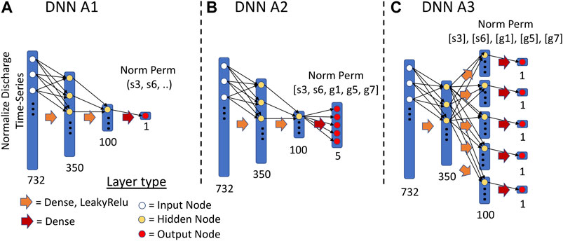
FIGURE 1. Illustration of three DNN architectures. (A) The DNN A1 architecture; (B) The DNN A2 architecture; (C) The DNN A3 architecture. The input to each of the models is the normalized discharge time-series data (see Sections 4.1 and 4.2). The output from DNN A1 is a single normalized permeability parameter. The outputs from DNN A2 and A3 are five normalized permeability parameters.

3 Study Site and Training Data Generation

To test the performance of the proposed DNNs in estimating subsurface properties from discharge data, we applied the method to a small catchment, the Rock Creek watershed, in Colorado (CO). Ensemble forward simulations were performed to provide sufficient training data for the DNNs that map the stream discharge hydrograph to the permeabilities of various soil and geologic layers. This section describes the study site, the forward watershed model implemented using the Advanced Terrestrial Simulator (ATS), and the generation of training data from ensemble ATS simulations.

3.1 Study Site: Rock Creek

Rock Creek is a small $\left(3{\text{km}}^2\right)$ primary catchment in the East River watershed near Crested Butte, CO. The watershed is a high alpine, snow dominated catchment, characterized as Dfb, or warm summer, humid continental climate on the Koppen classification system. It is characterized by majority aspen, meadow, and mixed conifer vegetation types, and receives approximately 70 cm of precipitation per year. This site is part of the Watershed Function Science Focus Area of the Department of Energy, and has a significant history of hydrologic studies on mountainous, primary watersheds (Carroll et al., 2018; Hubbard et al., 2018).

3.2 ATS Forward Model

ATS is an integrated, distributed hydrologic code that solves the diffusion wave approximation of the St. Vernant equations for surface flow coupled to Richards equation for flow in variably saturated porous media in the subsurface (Coon et al., 2019). This coupling is achieved through a continuous pressure, continuous flux approach described by Coon et al. (2020) and Painter et al. (2016). This code leverages the Mimetic Finite Difference method to ensure accurate, efficient solution of the equations, in mixed, conservative form [e.g., Celia et al. (1990)] on meshes that allow distorted, arbitrary polyhedra, including the triangular prisms used here. The resulting equations are solved using an implicit, backward Euler time integration scheme which is solved using the Nonlinear Krylov Acceleration approach of Carlson and Miller (1998); Calef et al. (2013) and preconditioned using the Boomer Algebraic Multigrid package in HYPRE (Falgout and Yang, 2002). This code has been benchmarked against a variety of hydrologic codes in Kollet et al. (2017), and is shown to be appropriate for solving problems of integrated hydrology (e.g., watersheds).

The baseline simulation was developed by using the Watershed Workflow package (Coon, 2020) to bring together a variety of data streams, delineate the catchment, and generate a variable resolution mesh with refined resolution at the stream network. Resolutions ranged from typical cell areas of 5,000 m² at the stream to 10,000 m² away from the stream network. This triangular surficial mesh was then elevated using Digital Elevation Model (DEM) from the National Elevation Dataset (NED) 9 m resolution dataset. In the work of Pribulick (2015), a base subsurface structure was defined by three stratigraphic layers–a soil layer of 1 m at the surface of the mesh, a near-surface geology layer 9 m thick below the soil layer, and a bedrock layer 20 m thick below the geologic layer. Based on the National Resources Conservation Service (NRCS) soils database, two soil types were identified and mapped within the soil layer. Using a surface geology dataset from the United States Geological Survey geological maps, three geologic material types were identified and mapped within the geologic layer. The spatial distribution of the soil and geological layers is demonstrated in Figure 2A. The vertical resolution of the mesh gradually increased from $\Delta z=5\text{cm}$ at the surface to 2 m at the 2 m depth, and it remained constant at 2 m until the bottom of the model domain at a depth of 30 m.

FIGURE 2

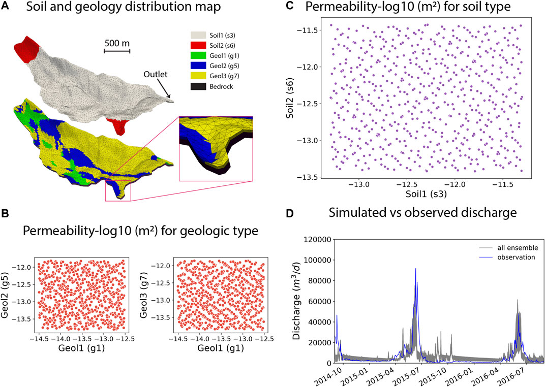
FIGURE 2. (A) Soil and geology distribution within the Rock Creek watershed. The zoom-in box shows the triangle meshes. (B) Permeability [log10 (m²)] realizations for three geologic types. (C) Permeability [log10 (m²)] realizations for two soil types. (D) Ensemble of simulated discharge hydrographs from 597 realizations compared with the observed discharge hydrograph.

The model was first run for 20,000 days with constant precipitation $\left(\sim 556\text{mm}/\text{yr}\right)$ and the permeabilities for all the soil and geological layers adopted from the work of Pribulick (2015) as the spin-up that resulted in steady state model outputs at the final timestep, which was then used as the initial condition for an 8-year transient simulation (2010 to 2017) driven by daily-averaged meteorological data from the DayMet (Thornton et al., 2016) dataset. The DayMet forcing is a $1\mathrm{km}$ raster that covers the entire North America with only three pixels over our modeling domain. Time series of precipitation, air temperature, incoming shortwave radiation, and relative humidity were mapped onto the mesh, and prescribed throughout the simulation. Additional setup/inputs required for ATS are described in the Supplementary Text S3.

To develop the training, validation and testing datasets for the DNNs, we completed an ensemble of 597 ATS transient simulations for the Rock Creek watershed, each simulation corresponded to a given set of soil and geology permeability parameters randomly generated from their probability distributions. Uniform distributions were assumed for all the parameters, with the lower and upper bounds chosen to be one order of magnitude below and above their values used in the baseline transient simulations. Quasi-Monte Carlo sampling method (Lemieux, 2009) was used to generate the permeability realizations shown in Figures 2B,C. The ensemble of simulated discharges in Figure 2D show reasonable match with the observed discharges at the outlet with RMSE ranging from 4.3 to 5.2 mm/day), which is a strong evidence for a reasonable conceptual model and sensitivity of the discharge to variations in soil and geologic layer permeabilities. We only used the discharge data from August 31, 2014 to August 31, 2016 to train the DNNs such that the trained model can be used to estimate the permeability of the real watershed from the limited field observation data available in this region during the same time window.

4 DNN Training

4.1 Data Preprocessing and Preparation

Prior to training the DNNs, the discharge data D was log-transformed and normalized via zero-mean and unit variance using the following equation:

$N\left(D\right)=\left[\ln \left(D\right)-\overline{\ln \left(D_t\right)}\right]/\sigma \left[\ln \left(D_t\right)\right],(1)$

where $\overline{\ln \left(D_t\right)}$ and $\sigma \left[\ln \left(D_t\right)\right]$ are the mean and standard deviation of the log-transformed discharge in the training dataset, respectively. Five of the permeability parameters were also log-transformed and normalized via zero-mean and unit variance using the same equation N, performed independently for each of them.

4.2 Training of DNNs

The DNNs were designed and implemented with the Keras python module (Chollet, 2015). In order to train the models, we divided the ensemble of 597 ATS runs into training, validation, and testing sets using roughly 70-15-15% divide (477, 60, 60 runs), respectively. Each run contains 732 daily measurements from August 31, 2014 to August 31, 2016, which were used as the input for all the DNNs. The DNN models were trained on the training set of 477 runs for 1,500 epochs with a batch size of 10, using mean-squared error (MSE) as the loss function and an Adam optimizer (Kingma and Ba, 2014). For each DNN type, we performed a hyperparameter search by varying the learning rate for training and the size of the layers (see Supplementary Table S1 for the combinations of learning rate and layer size). After the training was completed, each DNN model configuration was run on the validation set to choose the best model hyperparameters (i.e., model configuration) of a given DNN architecture. Each DNN configuration was trained using four different initialization seeds and results were averaged during validation. For the DNN A1 models, we trained separate models to estimate each of the five permeability parameters. Supplementary Table S2 shows the best hyperparameter combination for each model type based on the MSE on the validation set. Then, the best model configuration of each DNN architecture (e.g., DNN A1, A2, A3) was run on the testing set, and their performance was compared against each other.

4.3 Ensemble Smoother

We compared the DNNs against the ES approach in estimating permeabilities to assess the importance of dealing with nonlinearity between model inputs and outputs in inverse modeling. We followed a similar training-testing strategy when applying the ES method as used in the DNNs. We took the 537 realizations used in training and validation sets for DNNs as the prior ensembles for the permeabilities and modeled responses, then we perturbed each simulated hydrograph in the testing set (60 realizations in total) by adding random observation errors and used them as the synthetic observations, which were assimilated by the ES to generate posterior ensemble of permeabilities. The testing process yielded 60 sets of posterior permeability ensemble given an observation error, which is a hyperparameter for the ES approach. We considered a range of relative errors for discharge observations: 0.005, 0.01, 0.015, 0.02, 0.03, 0.05, and 0.1. For each observation error, we computed the correlation coefficient and root mean square error (RMSE) between the 60 synthetic true permeability and the corresponding 60 estimations from each of the 537 posterior realizations. We found that the ES trained with relative error of 0.05 performed the best in terms of both correlation coefficient and RMSE. More details about this analysis can be found in the Supplementary Text S2. Therefore, we chose the ES trained with a relative error of 0.05 for the comparison against the DNNs and for estimating the permeability from real observations.

5 Results and Discussion

5.1 Training Results of DNNs

Overall, we were able to successfully train the three DNN types to estimate the permeability parameters from the simulated stream discharge. As can be seen in the overall training loss for the DNN A3 model (Figure 3A), the DNN model learns to estimate the permeabilities during the training period. The overall and individual validation losses plateau before or around epoch 600 as shown in Figure 3. For the permeability of s6 (Figure 3C), its training loss continues to decrease after its validation loss plateaus, indicating an overfitting problem due to insufficient training data or lack of useful information in the discharge data to constrain the permeability. Similarly, the DNN A3 model also overfits on the g1 permeability (Figure 3D), but to a lesser extent as the validation loss is much closer to the training loss. No overfitting problems were found for the permeabilities of s3, g5, and g7 as their validation losses closely follows the training losses as seen in Figures 3B,E,F. The training and validation losses for the DNN A1 and DNN A2 models have similar performance and the figures are available in the Supplementary Figures S3, S4. Therefore, the overall overfitting of the DNNs can be mainly attributed to the overfitting on the s6 permeability, and to a lesser extent on the g1 permeability.

FIGURE 3

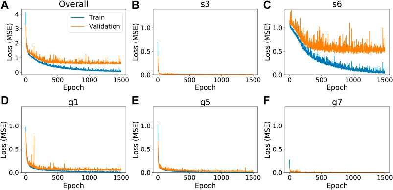
FIGURE 3. Training loss of the best DNN A3 model. The blue line is the loss from the training set and the orange line is the loss from the validations set. The x-axis is the epoch number. The y-axis is the model loss (MSE). (A) overall training loss of best DNN A3 model. The overall loss is the sum of the loss of the five permeability parameters (B–F); (B) training loss for the s3 permeability parameter; (C) training loss for the s6 permeability parameter; (D) training loss for the g1 permeability parameter; (E) training loss for the g5 permeability parameter; (F) training loss for the g5 permeability parameter.

On the training set, all the three DNN types perform very well in estimating the permeability parameters. As shown in Figure 4, the one-to-one plots between the permeabilities estimated by the DNN A3 model and the real permeabilities are distributed closely along the 1:1 lines. The DNN A1 and A2 models achieve similar levels of performance and their plots are available in the Supplementary Figures S5, S6, respectively. All three models yield $R^2$ values greater than 0.99 for the s3, g1, g5, and g6 permeabilities (see Supplementary Table S3). All three DNNs perform relatively worse in estimating the s6 permeability on the training set, as evidenced by more scatters drifted from the 1:1 line in Figure 4, resulting in $R^2$ values of about 0.96 from the DNN A2 and A3 models, and an $R^2$ of 0.89 from the DNN A1 model.

FIGURE 4

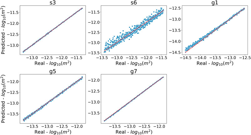
FIGURE 4. One-to-one plot of the DNN A3 model permeability estimation when compared to the real estimation for the training set. Each plot is the DNN A3 model estimation for the given permeability parameter. Each dot represents a realization from the training set of ensembles. The x-axis is the ${\log }_{10}$ real permeability value, the y-axis is the ${\log }_{10}$ estimated permeability value from the model. The red line is the one-to-one line.

5.2 Testing Results of DNNs

For the testing set, all the three DNN types perform very well in estimating the s3, g5, and g7 parameters, with $R^2$ values between the predicted and true permeabilities for all DNN models above 0.98. However, the $R^2$ drops to $\sim 0.93$ for the g1 permeability and below 0.6 for the s6 permeability (see Supplementary Table S4). The one-to-one scatter plots for DNN A3 in Figure 5 further demonstrates the disparity in estimation accuracy between the group of s3, g5, and g7 and the group of s6 and g1, which is similar to the training results with increased deviation from the exact 1:1 line. The one-to-one plots for the DNN A1 and DNN A2 models follow the same pattern and the plots are available in the Supplementary Figures S7, S8, respectively.

FIGURE 5

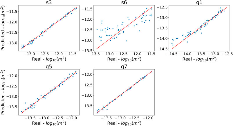
FIGURE 5. One-to-one plot for permeability estimated from the DNN A3 model against the true permeability in the testing set. Each plot is for a given permeability parameter, and each data point represents a realization from the testing set. The x-axis is the ${\log }_{10}$ real permeability value, the y-axis is the ${\log }_{10}$ estimated permeability value from the model. The red line is the one-to-one line.

The difficulty in estimating the s6 and g1 permeabilities might be explained by the small areas covered by these two soil/geologic layers (Figure 2A) and their distances from the outlet where the discharges are measured. Thus, they may not contribute as much to the simulated discharge compared to the other parameters. In other words, the simulated discharges are not as sensitive to the s6 and g1 permeabilities, and consequently the discharges at the outlet are not sufficiently informative for estimating the s6 and g1 permeabilities.

The performance of all three DNN architectures on the testing set was compared using the squared errors between the estimated and true log10-transformed permeabilities. Figure 6 shows the three quartiles and ranges of the squared errors calculated from the 60 realizations in the testing set using boxplots, while their means and standard deviations are provided in Supplementary Table S4. All the DNN architectures yield very similar results in terms of the statistics of the squared errors for all the parameters. Their mean squared errors (MSEs) differ by less than $1.1\times {10}^{-4}$ for the g7 permeability, around $4.8\times {10}^{-4}$ for the s3 permeability, and within $1.3\times {10}^{-3}$ for the g5 permeability. Overall, the DNN A1 models slightly outperform the DNN A2 and DNN A3 models in terms of the means and medians of squared errors provided in Figure 6 and Supplementary Table S4. The MTL models show slight improvement over the STL models in MSE and $R^2$ for the s6 permeability, suggesting the potential for the less sensitive parameters to benefit from the joint features developed in MTL models at little or no expense to the estimation accuracy of other parameters. The performance difference between the DNN A2 and A3 models appears negligible. Thus, in this case study, it may not be necessary to add additional model complexity using the sub-networks to develop parameter-specific features.

FIGURE 6

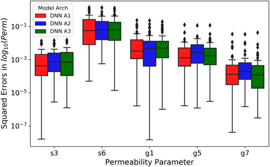
FIGURE 6. Box plot of the squared error of the DNNs on the testing set. The x-axis is the permeability parameter. The y-axis is the squared error of the estimated ${\log }_{10}$ of the permeability parameter compared to their true values. The y-axis is plotted in log-scale for showing differences spanning over several orders of magnitude. The results for different DNN architectures are represented by the colors filling the box plots.

5.3 Estimation Sensitivity to Observation Errors

To assess how sensitive the DNN-based parameter estimation is to observation errors in the data used for inverse modeling, we randomly selected a realization from the testing set and generated 100 realizations of noisy observed discharge time series $\left({\mathbf{d}}_{\mathbf{n}}\right)$ by adding random observation errors to the simulated discharges $\left(\mathbf{d}\right)$, i.e.,

${\mathbf{d}}_{\mathbf{n}}=\mathbf{d}+\mathrm{ϵ}\ast \mathbf{d}\ast \mathbf{r},(2)$

where $\mathbf{r}$ is a vector of the same size as $\mathbf{d}$ composed of random samples drawn from a standard normal (Gaussian) distribution with a mean of 0 and a standard deviation of 1, and ϵ is the standard deviation of the noise, which is usually taken as 1/3 of the observation error. For this study, we set $\mathit{ϵ}=0.0166$ for a 5% observation error. Then, we obtained 100 realizations of estimated permeability set from each of the DNN model types with the best configuration (the same ones used in Section 5.2) from the 100 realizations of noisy discharges. The variability in estimated permeabilities are shown in boxplots in Figure 7. It is observed across all the DNN model types that the parameters that can be accurately estimated (i.e., s3, g5, and g7) from the discharge data show more robust performance under the presence of the observation errors, whereas those that are estimated less successfully (i.e., s6 and g1) are also more vulnerable to the observation errors.

FIGURE 7

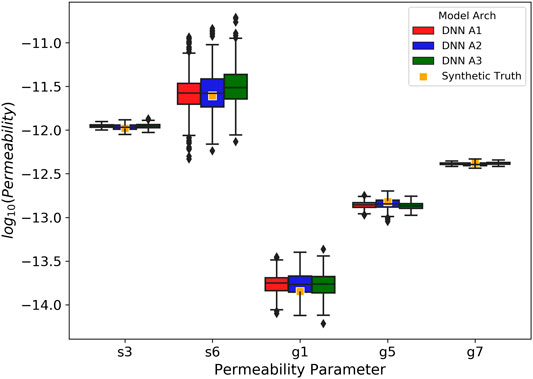
FIGURE 7. Sensitivity of model types to noise added to the simulated discharge for ensemble 537. The boxplots represent the distribution of the ${\log }_{10}$ estimated permeability value from the 100 noisy discharge vectors. The yellow square dot are the synthetic permeability values for the simulation (ensemble 537).

As discussed in Section 5.2, it is highly likely that there is less information available in the discharge data for estimating parameters with smaller spatial coverage, which consequently limits DNNs in their ability to generalize beyond the training data. The observation error further contaminates the useful information (i.e., signal) in the data, thus exacerbating the estimating inaccuracy.

5.4 Comparison With Ensemble Smoother

We compared the performance of DNN-based methods against the ES method (with relative error of 0.05) in estimating the permeability from the same discharge data using the squared errors of the estimated permeability on the testing set, as shown in Figure 8. To ensure a fair comparison, for each realization in the testing set, we generated 100 noisy discharge time series assuming a 5% observation error, which led to 100 instances of estimated permeability set that are compared to their corresponding synthetic truth with squared errors calculated. Therefore, each boxplot in Figure 8 associated with the DNN methods was generated from 6,000 samples of squared errors, whereas that for the ES method was generated from 32,220 samples because each testing realization has an ensemble of 537 posterior estimations. The comparison shows that the DNNs significantly outperform the ES with much smaller squared errors for all the five permeabilities. The MSE across all five permeabilities for the DNNs (0.0568 for DNN A1, 0.051 for DNN A2, and 0.045 for DNN A3) is an order of magnitude smaller compared to the MSE for the ES method (0.634). Therefore, DNNs are promising alternatives for inverse modeling, especially for using indirect data that are nonlinearly related to the parameters of interest.

FIGURE 8

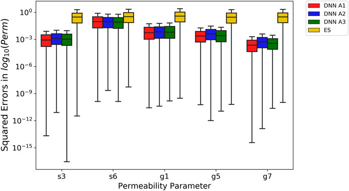
FIGURE 8. Box plots of squared errors on permeabilities estimated by DNNs and ES for the testing set using relative observation error 0.05. The x-axis is the permeability parameter. The y-axis is the squared errors of the ${\log }_{10}$-transformed permeability parameters. The y-axis is shown in log-scale. The boxplots are filled with different colors corresponding to different estimation methods.

Additionally, we investigated the amount of training data needed to achieve a similar level of accuracy using the full amount of training data for the DNNs and the ES approach. We trained the three DNNs using 50, 100, 200, and 300 realizations from the training set with the same hyperparameters listed in Supplementary Table S2. Then, we performed the ES-based estimations with a relative error of 0.05 with the same four training sets of various sizes. Finally, permeabilities on the testing set were estimated using the DNNs trained on different amount of data and the ES of various ensemble sizes and compared. Both sets of estimations assumed a relative observation error of 5%. As shown in Figures 9A–C that the performance of DNNs keeps improving with the increasing amount of training data increases. Nevertheless, the gain in performance diminishes when the training data size is increased from 300 to 477. Thus, we consider 300 realizations as sufficient for achieving good training results for the DNNs in this case study. The ES approach, on the other hand, does not show as much improvement in estimation accuracy when increasing the ensemble size (Figure 9D). Interestingly, the DNNs trained with 50 realizations yield a lower MSE for all the s3, g1, g5, and g7 permeability parameters than all of the ES variations, while achieving equivalent performance for the s6 permeability. Therefore, the DNNs may require less training information to achieve equivalent or better performance than the ES. Moreover, the DNNs can more effectively utilize the information in larger training dataset than the ES approach to capture nonlinear relationships.

FIGURE 9

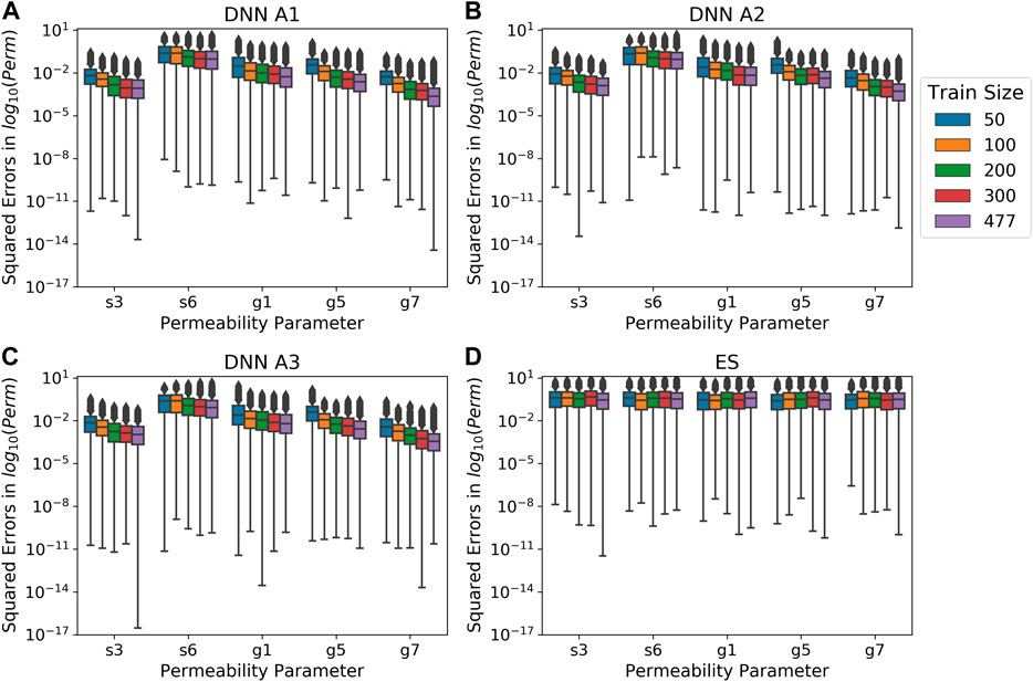
FIGURE 9. Box plots of squared errors on permeabilities estimated by DNNs and ES for the testing set using relative observation errors of 0.05 with different training data sizes. The x-axis is the permeability parameter. The y-axis is the squared errors of the ${\log }_{10}$-transformed permeability parameters. The y-axis is shown in log-scale. Each color represents a number of realizations used to train the DNNs or ES (50, 100, 200, 300, 477). (A) the squared errors for the DNN A1 model; (B) the squared errors for the DNN A2 model; (C) the squared errors for the DNN A3 model; (D) the squared errors for the ES.

We also compared the computation times needed for both methods. The computational cost for DNN models is spent on both the training and prediction phases, whereas the ES approach does not have an explicit training phase. We were able to perform the DNN-based and ES-based inversions on laptops without involving the Graphics Processing Unit (GPU) or parallel computing. The DNN A1 and DNN A2 models finished training for 1,500 epochs in under 2 min. The DNN A3 finished training in just over 5 min. For estimating the permeabilities from a single time series of stream discharge, the DNNs took less than 0.4 ms on average. When estimating all 60 stream discharges in the testing set, DNNs A1, DNN A2, and DNN A3 took 0.87, 0.89, and 1.17 ms, respectively, on average. For estimating the permeability for a single discharge time series, the ES took approximately 40 ms to update the permeability ensemble by assimilating the corresponding discharge observations through matrix operations. The computational costs spend on the inversion using either of the methods are negligible compared to the computing resources required to generate the training, validation and tesing datasets from ensemble ATS simulations, which were approximately 324,768 cpu hours using the supercomputing resources at the National Energy Research Scientific Computing Center (NERSC).

5.5 Permeability Estimation From Observed Discharge for Real Systems

After achieving the adequate estimation performance on training and testing the DNNs, we moved forward with estimating the soil and geologic permeability parameters of the Rock Creek catchment from the real observed discharge (Figure 2D) using the DNNs trained and tested in Section 5.2. We generated 100 realizations of noisy discharge time series from the real observed discharge assuming a relative observation error of 5%. The ensembles of the estimated permeability parameters by DNNs were used to generate the boxplots in Figure 10, compared against the posterior estimates from the ES approach with a relative observation error of 5%. Note that the prior boxplots were generated from the prior parameter ensemble for the ES approach, which was also used as the DNN training dataset. It can be observed from Figure 10 that the DNN estimations for the s3 and g7 permeabilities are distributed in the similar ranges as in their training data, while the DNN estimations for the g5, g1 and s6 permeabilities are significantly shifted away from their ranges in the training dataset. The variability in results obtained from different DNN types is substantially greater for the g5, g1 and s6 parameter group than the s3 and g7 group, which is consistent with the difference in their sensitivity to the discharge time series as revealed during the training and testing stages. Thus, the estimated permeabilities for s3 and g7 are likely more accurate (i.e., reasonable) than those for g5, g1 and s6.

FIGURE 10

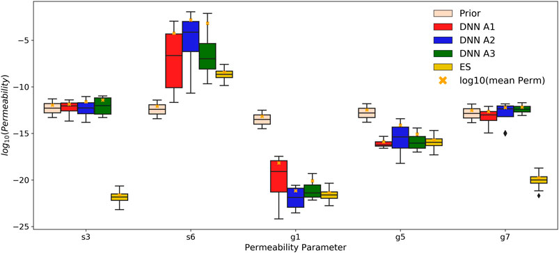
FIGURE 10. Permeability estimations from the observed discharges from the DNNs and the ES using relative observation error of 0.05. The peach-colored boxplots are the prior distributions for each permeability parameter. The gold-colored boxplots are the distribution of permeability estimations from the ES. Each of the remaining colored boxplots is the corresponding distributions of DNN estimations. The orange crosses are the ${\log }_{10}$-transformed mean permeability value for the corresponding distribution.

Figure 10 also demonstrates that the ES approach yielded vastly different estimations from the DNN models, except for the g5 permeability, with relatively tighter distributions. The considerable differences between the prior and posterior distributions in parameters suggest that the estimations are extrapolated from the training/prior data for this real application, which is related to the fact that the ensemble of the simulated hydrographs failed to encapsulate the observed hydrograph in major recession periods as shown in Figure 2D. DNNs appear to provide more realistic estimations for the s3 and g7 permeability than the ES. The s3 permeability estimated by the ES is unrealistically low for soils, even lower than the geologic layers, which may be caused by extrapolation errors based on linearized relation between model parameters and outputs. DNNs, on the other hand, are better able to generalize in this case by capturing the nonlinear relationships. To evaluate how the estimated permeabilities change the model predictions of the hydrograph at the outlet, we randomly selected 30 realizations from the ensembles of permeabilities estimated by the DNN A1 and the ES to generate updated ensembles of predicted hydrographs, which were then compared to the observations to assess the improvement in model performance. We encountered numerical model convergence issues for some permeability combinations with substantial contrast between the low-permeability and high-permeabilities layers. Thus, not all simulations were completed within the assigned wall clock time. The ensemble simulation results in Figure 11 contain nine and five sets of completed simulations for the DNN A1 and the ES, respectively. Although the ensemble sizes of model runs may not be sufficient for representing the full range of uncertainty in the updated model predictions, we expect them to adequately represent the mean model behaviors. Overall, the permeabilities estimated by DNN A1 lead to much improved prediction during year 2015 as compared to the prior predictions in Figure 2D, whereas they cause considerable overpredictions in peak discharges during year 2016. In contrast, the models with the permeabilities estimated by the ES consistently overpredict the discharges owing to the unrealistically low permeability estimated for s3. It is worth noting that none of the simulated hydrographs reproduces the same level of inter-annual variability manifested in the real observations, which implies potential deficiencies in the numerical model representation of the real system. Further investigations are needed to identify additional processes and parameters that may contribute to such inter-annual variability.

FIGURE 11

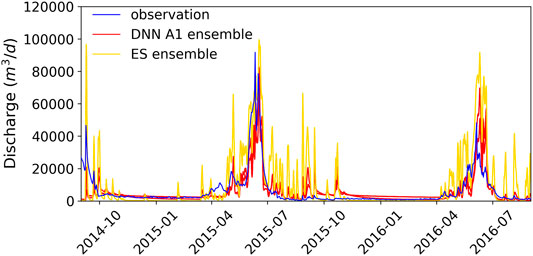
FIGURE 11. Comparison between the observed discharge and the predicted discharge from ATS using the estimated permeability values from the DNN A1 and ES, respectively.

6 Conclusion

In this paper, we developed a DNN-based inversion method to estimate permeabilities of multiple soil and geologic layers within a watershed from the observed stream discharge time series. We successfully trained DNNs to map from the stream discharges to the permeability set using the training/validation/testing data generated through the ensemble watershed simulations. In doing so, we found that the accuracy and robustness of DNN-based estimations are influenced by the relevant information content contained in the observation data with respect to the parameters. In the watershed system we studied, permeability for soil and geologic layers with larger spatial coverage can be estimated more accurately from the observed discharge data, and their estimations were more robust to observation errors.

In comparing the parameters estimated by the DNNs and the traditional ES method from the same observation data, we found that the DNNs consistently outperformed the ES algorithm. On the testing set, the DNNs achieved an overall MSE an order of magnitude lower than the ES method. The DNNs is more effective in utilizing the information provided by larger training dataset than the ES approach. By capturing the nonlinear relationships between the model inputs and outputs through multiple layers of neurons, DNNs yielded more realistic permeability estimations for the real watershed system, leading to improved match between model predicted and observed stream discharges. However, improving the permeability used in the model alone does not enable the models to capture the inter-annual variability in the discharges, future work is needed to identify additional processes and parameters that may contribute to the unresolved inter-annual variability in system responses.

Note that the accuracy of DNN-based estimation of permeability will be impacted by the accuracy of the mapped distributions of soil and geologic layers, which directly impacts how well a numerical model can represent a real system. During training, the DNNs learn to estimate the permeabilities from the simulated stream discharge for that given distribution map of soil and geologic formation types. Therefore, a less accurate distribution map will result in less accurate estimations of the permeabilities for the watershed, leading to biases that cannot be resolved by the inversion method. A facies-based approach [e.g., Song et al. (2019)] can be adopted to estimate the distribution of soil types and geologic layers along with their permeabilities.

Our study has demonstrated that the DNNs can potentially be a powerful tool to estimate parameters from indirect, relevant observations. The success in linking permeability with stream discharges using DNNs presents new opportunities to improve the subsurface characterization of large-scale watersheds, which has been limited by scarce subsurface characterization and observation data. Our work also paves the way for developing more general model calibration strategies that involve multiple parameters and multiple types of observation data for complex systems. Our next step is to expand the study to assist the multi-process modeling for larger watersheds with more complex subsurface structures. New DNN architectures with deeper and bigger networks might be required to deal with the increasing dimensionality in both model inputs and outputs. Substantial computational resources may also be required to generate sufficient training data for the DNN models if high-resolution distributed models are used.

Data Availability Statement

The datasets presented in this study can be found in online repositories. The names of the repository/repositories and accession number(s) can be found on ESS-Dive: https://doi.org/10.15485/1756193.

Author Contributions

XC and EC conceived and designed the study with input from SLP and ETC. EC lead the writing of the manuscript, developed DNNs architectures and performed DNNs analysis. ETC and SLP developed the reference case forward simulation of Rock Creek using ATS. PS conducted the ensemble of numerical simulations using ATS and provided data inputs for DNNs training. PJ performed the ensemble smoother. EC provided model related details and background information. SLP, JDM, YL, and ETC provided guidance and overall direction and participated in the interpretation of results. All authors provided critical feedback and inputs to the manuscript.

Funding

This work was funded by the ExaSheds project, which was supported by the United States Department of Energy, Office of Science, Office of Biological and Environmental Research, Earth and Environmental Systems Sciences Division, Data Management Program, under Award Number DE-AC02-05CH11231.

Conflict of Interest

The authors declare that the research was conducted in the absence of any commercial or financial relationships that could be construed as a potential conflict of interest.

Acknowledgments

The authors are grateful to Ahmad Jan for helping with model setup for the reference case ATS model of Rock Creek and to Zhufeng Fang for helping developed the reference case forward simulation of Rock Creek using ATS. This research used resources of the National Energy Research Scientific Computing Center, a DOE Office of Science User Facility supported by the Office of Science of the United States Department of Energy under contract DE-AC02-05CH11231. Pacific Northwest National Laboratory is operated for the DOE by Battelle Memorial Institute under contract DE-AC05-76RL01830. Oak Ridge National Laboratory is managed by UT-Battelle, LLC for the U.S. Department of Energy under Contract Number DE-AC05-00OR22725. Los Alamos National Laboratory is operated by Triad National Security, LLC, for the National Nuclear Security Administration of U.S. Department of Energy (Contract No. 89233218CNA000001). This paper describes objective technical results and analysis. Any subjective views or opinions that might be expressed in the paper do not necessarily represent the views of the United States Department of Energy or the United States Government. This manuscript has been co-authored by UT-Battelle, LLC under Contract No. DE-AC05-00OR22725 with the U.S. Department of Energy. The United States Government retains and the publisher, by accepting the article for publication, acknowledges that the United States Government retains a non-exclusive, paidup, irrevocable, world-wide license to publish, or reproduce the published form of this manuscript, or allow others to do so, for United States Government purposes. The Department of Energy will provide public access to these results of federally sponsored research in accordance with the DOE Public Access Plan (http://energy.gov/downloads/doe-public-access-plan).

Supplementary Material

The Supplementary Material for this article can be found online at: https://www.frontiersin.org/articles/10.3389/feart.2021.613011/full#supplementary-material.

References

Ala-aho, P., Soulsby, C., Wang, H., and Tetzlaff, D. (2017). Integrated surface-subsurface model to investigate the role of groundwater in headwater catchment runoff generation: a minimalist approach to parameterisation. J. Hydrol. 547, 664–677. doi:10.1016/j.jhydrol.2017.02.023

CrossRef Full Text | Google Scholar

ASCE Task Committee (2000). Artificial neural networks in hydrology. ii: hydrologic applications. J. Hydrol. Eng. 5, 124–137. doi:10.1061/(ASCE)1084-0699(2000)5:2(124)

CrossRef Full Text | Google Scholar

Bailey, R., and Baù, D. (2010). Ensemble smoother assimilation of hydraulic head and return flow data to estimate hydraulic conductivity distribution. Water Resour. Res. 46, W12543. doi:10.1029/2010WR009147

CrossRef Full Text | Google Scholar

Baxter, J. (1997). A Bayesian/information theoretic model of learning to learn via multiple task sampling. Mach. Learn. 28, 7–39. doi:10.1023/a:1007327622663

CrossRef Full Text | Google Scholar

Calef, M. T., Fichtl, E. D., Warsa, J. S., Berndt, M., and Carlson, N. N. (2013). Nonlinear Krylov acceleration applied to a discrete ordinates formulation of the k-eigenvalue problem. J. Comput. Phys. 238, 188–209. doi:10.1016/j.jcp.2012.12.024

CrossRef Full Text | Google Scholar

Canchumuni, S. W. A., Emerick, A. A., and Pacheco, M. A. C. (2019). Towards a robust parameterization for conditioning facies models using deep variational autoencoders and ensemble smoother. Comput. Geosci. 128, 87–102. doi:10.1016/j.cageo.2019.04.006

CrossRef Full Text | Google Scholar

Carlson, N. N., and Miller, K. (1998). Design and application of a gradient-weighted moving finite element code I: in one dimension. SIAM J. Sci. Comput. 19, 728–765. doi:10.1137/S106482759426955X

CrossRef Full Text | Google Scholar

Carrera, J., Alcolea, A., Medina, A., Hidalgo, J., and Slooten, L. J. (2005). Inverse problem in hydrogeology. Hydrogeol. J. 13, 206–222. doi:10.1007/s10040-004-0404-7

CrossRef Full Text | Google Scholar

Carroll, R. W. H., Bearup, L. A., Brown, W., Dong, W., Bill, M., and Willlams, K. H. (2018). Factors controlling seasonal groundwater and solute flux from snow-dominated basins. Hydrol. Process. 32, 2187–2202. doi:10.1002/hyp.13151

CrossRef Full Text | Google Scholar

Caruana, R. (1997). Multitask learning. Mach. Learn. 28, 41–75. doi:10.1023/a:1007379606734

CrossRef Full Text | Google Scholar

Celia, M. A., Bouloutas, E. T., and Zarba, R. L. (1990). A general mass-conservative numerical solution for the unsaturated flow equation. Water Resour. Res. 26, 1483–1496. doi:10.1029/WR026i007p01483

CrossRef Full Text | Google Scholar

Chen, X., Hammond, G. E., Murray, C. J., Rockhold, M. L., Vermeul, V. R., and Zachara, J. M. (2013). Application of ensemble-based data assimilation techniques for aquifer characterization using tracer data at hanford 300 area. Water Resour. Res. 49, 7064–7076. doi:10.1002/2012WR013285

CrossRef Full Text | Google Scholar

Chen, X., Lee, R. M., Dwivedi, D., Son, K., Fang, Y., Zhang, X., et al. (Forthcoming 2020). Integrating field observations and process-based modeling to predict watershed water quality under environmental perturbations. J. Hydrol. doi:10.1016/j.jhydrol.2020.125762

CrossRef Full Text | Google Scholar

Chen, Y., and Oliver, D. S. (2013). Levenberg-Marquardt forms of the iterative ensemble smoother for efficient history matching and uncertainty quantification. Comput. Geosci. 17, 689–703. doi:10.1007/s10596-013-9351-5

CrossRef Full Text | Google Scholar

Chollet, F., et al. (2015). Keras. Available at: https://keras.io.

Google Scholar

Clark, M. P., Rupp, D. E., Woods, R. A., Zheng, X., Ibbitt, R. P., Slater, A. G., et al. (2008). Hydrological data assimilation with the ensemble Kalman filter: use of streamflow observations to update states in a distributed hydrological model. Adv. Water Resour. 31, 1309–1324. doi:10.1016/j.advwatres.2008.06.005

CrossRef Full Text | Google Scholar

Coon, E. (2020). Watershed workflow: a suite of tools for generating hyper-resolution hydrology simulations. Oak Ridge National Laboratory, Tech. Rep. Available at: https://github.com/ecoon/watershed-workflow/.

Google Scholar

Coon, E., Moulton, J., Kikinzon, E., Berndt, M., Manzini, G., Garimella, R., et al. (2020). Coupling surface and subsurface flow in complex soil structures using mimetic finite differences. Adv. Water Resour. 144, 103701. doi:10.1016/j.advwatres.2020.103701

CrossRef Full Text | Google Scholar

Coon, E., Svyatsky, D., Jan, A., Kikinzon, E., Berndt, M., Atchley, A., et al. (2019). Advanced terrestrial simulator. [Computer Software]. doi:10.11578/dc.20190911.1

CrossRef Full Text | Google Scholar

Doherty, J. (2010). Pest user-manual: model-independent parameter estimation. 5th Edn. Brisbane, QLD, Australia: Watermark Numerical Computing.

Google Scholar

Emerick, A. A., and Reynolds, A. C. (2013). Ensemble smoother with multiple data assimilation. Comput. Geosci. 55, 3–15. doi:10.1016/j.cageo.2012.03.011

CrossRef Full Text | Google Scholar

Evensen, G. (2018). Analysis of iterative ensemble smoothers for solving inverse problems. Comput. Geosci. 22, 885–908. doi:10.1007/s10596-018-9731-y

CrossRef Full Text | Google Scholar

Evensen, G. (1994). Sequential data assimilation with a nonlinear quasi-geostrophic model using Monte Carlo methods to forecast error statistics. J. Geophys. Res. 99, 10143–10162. doi:10.1029/94JC00572

CrossRef Full Text | Google Scholar

Evensen, G. (2003). The Ensemble Kalman Filter: theoretical formulation and practical implementation. Ocean Dyn. 53, 343–367. doi:10.1007/s10236-003-0036-9

CrossRef Full Text | Google Scholar

Falgout, R. D., and Yang, U. M. (2002). “Hypre: a library of high performance preconditioners,” in Computational science—ICCS 2002 lecture notes in computer science. Editors P. M. A. Sloot, A. G. Hoekstra, C. J. K. Tan, and J. J. Dongarra (Berlin, Heidelberg, Germany: Springer), 632–641.

CrossRef Full Text | Google Scholar

Hubbard, S. S., Williams, K. H., Agarwal, D., Banfield, J., Beller, H., Bouskill, N., et al. (2018). The East River, Colorado, watershed: a mountainous community testbed for improving predictive understanding of multiscale hydrological-biogeochemical dynamics. Vadose Zone J. 17, 180061. doi:10.2136/vzj2018.03.0061

CrossRef Full Text | Google Scholar

Kingma, D. P., and Ba, J. (2014). Adam: a method for stochastic optimization. arXiv preprint arXiv:1412.6980.

Google Scholar

Kollet, S., Sulis, M., Maxwell, R. M., Paniconi, C., Putti, M., Bertoldi, G., et al. (2017). The integrated hydrologic model intercomparison project, IH-MIP2: a second set of benchmark results to diagnose integrated hydrology and feedbacks. Water Resour. Res. 53, 867–890. doi:10.1002/2016WR019191

CrossRef Full Text | Google Scholar

Lemieux, C. (2009). “Monte Carlo and quasi-Monte Carlo sampling,” in Springer series in statistics. Editors P. Bühlmann, P. Diggle, U. Gather, and S. Zeger (New York, NY: Springer).

Google Scholar

Mo, S., Zabaras, N., Shi, X., and Wu, J. (2019). Deep autoregressive neural networks for high‐dimensional inverse problems in groundwater contaminant source identification. Water Resour. Res. 55, 3856–3881. doi:10.1029/2018WR024638

CrossRef Full Text | Google Scholar

Moradkhani, H., Sorooshian, S., Gupta, H. V., and Houser, P. R. (2005). Dual state-parameter estimation of hydrological models using ensemble Kalman filter. Adv. Water Resour. 28, 135–147. doi:10.1016/j.advwatres.2004.09.002

CrossRef Full Text | Google Scholar

Oyebode, O., and Stretch, D. (2018). Neural network modeling of hydrological systems: a review of implementation techniques. Nat. Resour. Model. 32 (1), e12189. doi:10.1002/nrm.12189

CrossRef Full Text | Google Scholar

Painter, S. L., Coon, E. T., Atchley, A. L., Berndt, M., Garimella, R., Moulton, J. D., et al. (2016). Integrated surface/subsurface permafrost thermal hydrology: model formulation and proof-of-concept simulations. Water Resour. Res. 52, 6062–6077. doi:10.1002/2015WR018427

CrossRef Full Text | Google Scholar

Raghu, M., Poole, B., Kleinberg, J., Ganguli, S., and Sohl-Dickstein, J. (2017). “On the expressive power of deep neural networks,” in Proceedings of the 34th international conference on machine learning (PMLR), Sydney, NSW, Australia, August 6-11, 2017. Editors D. Precup, and Y. W. Teh (Sydney, NSW: International Convention Centre), Vol. 70, 2847–2854.

Google Scholar

Scanlon, T. M., Raffensperger, J. P., Hornberger, G. M., and Clapp, R. B. (2000). Shallow subsurface storm flow in a forested headwater catchment: observations and modeling using a modified TOPMODEL. Water Resour. Res. 36, 2575–2586. doi:10.1029/2000WR900125

CrossRef Full Text | Google Scholar

Shen, C. (2018). A transdisciplinary review of deep learning research and its relevance for water resources scientists. Water Resour. Res. 54, 8558–8593. doi:10.1029/2018WR022643

CrossRef Full Text | Google Scholar

Song, X., Chen, X., Ye, M., Dai, Z., Hammond, G., and Zachara, J. M. (2019). Delineating facies spatial distribution by integrating ensemble data assimilationand indicator geostatistics with level‐set transformation. Water Resour. Res. 55, 2652–2671. doi:10.1029/2018WR023262

CrossRef Full Text | Google Scholar

Pribulick, C. (2015). Propagating climate and vegetation change through the hydrologic cycle in a mountain headwaters catchment. MS thesis (Hydrology). Golden (CO): Colorado School of Mines.

Google Scholar

Thornton, P., Thornton, M., Mayer, B., Wei, Y., Devarakonda, R., Vose, R., et al. (2016). Data from: Daymet: daily surface weather data on a 1-km grid for North America Artwork size: 711509.8892839993 MB medium: NetCDF publisher: ORNL distributed active archive. Version 3, 711509.8892839993 MB 10.3334/ORNLDAAC/1328 Center Version Number: 3.4.

Google Scholar

van Leeuwen, P. J., and Evensen, G. (1996). Data assimilation and inverse methods in terms of a probabilistic formulation. Mon. Wea. Rev. 124, 2898–2913. doi:10.1175/1520-0493(1996)124<2898:DAAIMI>2.0.CO;2

CrossRef Full Text | Google Scholar

Vogt, C., Marquart, G., Kosack, C., Wolf, A., and Clauser, C. (2012). Estimating the permeability distribution and its uncertainty at the EGS demonstration reservoir Soultz-sous-Forêts using the ensemble Kalman filter. Water Resour. Res. 48, W08517. doi:10.1029/2011WR011673

CrossRef Full Text | Google Scholar

Wen, X.-H., and Chen, W. H. (2006). Real-time reservoir model updating using ensemble Kalman filter with confirming option. SPE J. 11, 431–442. doi:10.2118/92991-PA

CrossRef Full Text | Google Scholar

Zheng, Q., Zhang, J., Xu, W., Wu, L., and Zeng, L. (2019). Adaptive multifidelity data assimilation for nonlinear subsurface flow problems. Water Resour. Res. 55, 203–217. doi:10.1029/2018WR023615

CrossRef Full Text | Google Scholar