Lake Inflow Simulation Using the Coupled Water Balance Method and Xin’anjiang Model in an Ungauged Stream of Chaohu Lake Basin, China

Introduction

Water resources are of significance to maintain daily life because they not only provide directly available water resources for households, industry, and agriculture but also play a key role in maintaining healthy ecosystems (Li et al., 2017; Yang et al., 2020; Yu et al., 2020). Therefore, the available quantity should be calculated accurately as possible. In general, however, inflow observation data cannot be obtained directly in many lake/reservoir basins (Mohebzadeh and Fallah, 2019), especially in the areas where hydrological measurement stations have been poorly developed.

In the inflow studies of lake/reservoir basins, abundant observation data of water level and the relationship of water level and capacity of lake/reservoir make it possible to use the water balance method to calculate the lake/reservoir inflow (Deng et al., 2015; Gal et al., 2016). In this method, however, the estimated reliable inflow is a great challenge because the detailed daily water consumption data, including agricultural water, industrial water, domestic water, infiltration, etc., is difficult to obtain accurately. The results of daily lake/reservoir inflows calculated by the water balance method may be unreasonable and even negative values. In this context, the coupling of the water balance method and the hydrological model is needed to study the lake/reservoir inflows, in which flood events observations (estimated by the water balance method and called true inflows) were used to calibrate the hydrological model.

The hydrologic model used in this study is the Xin’anjiang model, which has emerged as a particularly promising method of dealing with complex hydrological phenomena due to the simple model structure (Bai et al., 2017), the clear physical meaning of the parameters (Lü et al., 2013), the well-defined model calibration procedure (Bai et al., 2017), and model development ability (Lin et al., 2014) following its first reported application to hydrological modeling problems by Zhao (1984). Meanwhile, the Xin’anjiang model has been widely applied in humid and semi-humid regions in China (Lü et al., 2013; Lin et al., 2014). In the model, although some insensitive parameters can be preset or estimated based on implementation experience, the sensitive parameters must be calibrated based on continuous historical streamflow data. In this study, the single objective particle swarm optimization (SOPSO) method, which is a population-based optimization technique proposed by Eberhart and Kennedy (1995), was added to the Xin’anjiang model to find the optimal parameters of the coupled model.

However, the SOPSO method becomes invalid because the observed daily inflow data, calculated by the flood events using the water balance method, is discontinuous. Thus, an improved SOPSO (I-SOPSO) method was used to calibrate hydrological model parameters, in which the daily precipitation data input by the Xin’anjiang model is sequentially read, but the inflows of the selected flood events (calculated by water balance method) are only read as the observed inflow data. Meanwhile, the maximum weighted average Nash-Sutcliffe efficiency (WANSE) of selected flood events is used as the objective function to minimize the error in estimating the goodness-of-fit between observed and simulated values. The advantage of the method is that it not only considers the impact of the previous precipitation and reduces the influence of anthropogenic activities, especially irrigation activities, but also can simulate the long-series daily lake/reservoir inflow, which is an important factor to consider in water resources decision-making (Yun et al., 2018).

Existing reservoir inflow simulation models and water balance methods in the area lacking hydrological measurement stations become limited due to the lack of a series of daily time scale reservoir inflow data. Thus, this paper attempt to solve this problem by coupling the water balance method with the Xin’anjiang model and applying the result to the Chaohu Lake Basin where hydrological stations have been poorly developed. The objective entails the following tasks: (1) determining typical hydrological years; (2) calculating the lake inflows of selected flood events; (3) finding the optimal parameters of coupled model; and (4) simulating the lake inflows of long-series. The results of the hydrological characteristics of the typical years of Chaohu Lake Basin will be of great significance for further studying the migration and diffusion of suspended matter in lakes, improving the ecological environment of lakes, and water resource planning and management.

Study Area and Data

Chaohu Lake, the fifth largest freshwater lake in China, is located in the central region of Anhui Province between the Yangtze and Huaihe. Also, Chaohu Lake Watershed is in the route of the Yangtze River Huaihe River water transfer project in China (Cao et al., 2018). Chaohu Lake Watershed can be divided into two large sub-basins, i.e., Upper Chaohu Lake Watershed and Lower Chaohu Lake Watershed. Upper Chaohu Lake Watershed is the study area of this paper, which is between latitudes 30°59′–32°9′ N and longitudes 116°23′–117°59′ E with a drainage area of 9153 km² (Figure 1).

FIGURE 1

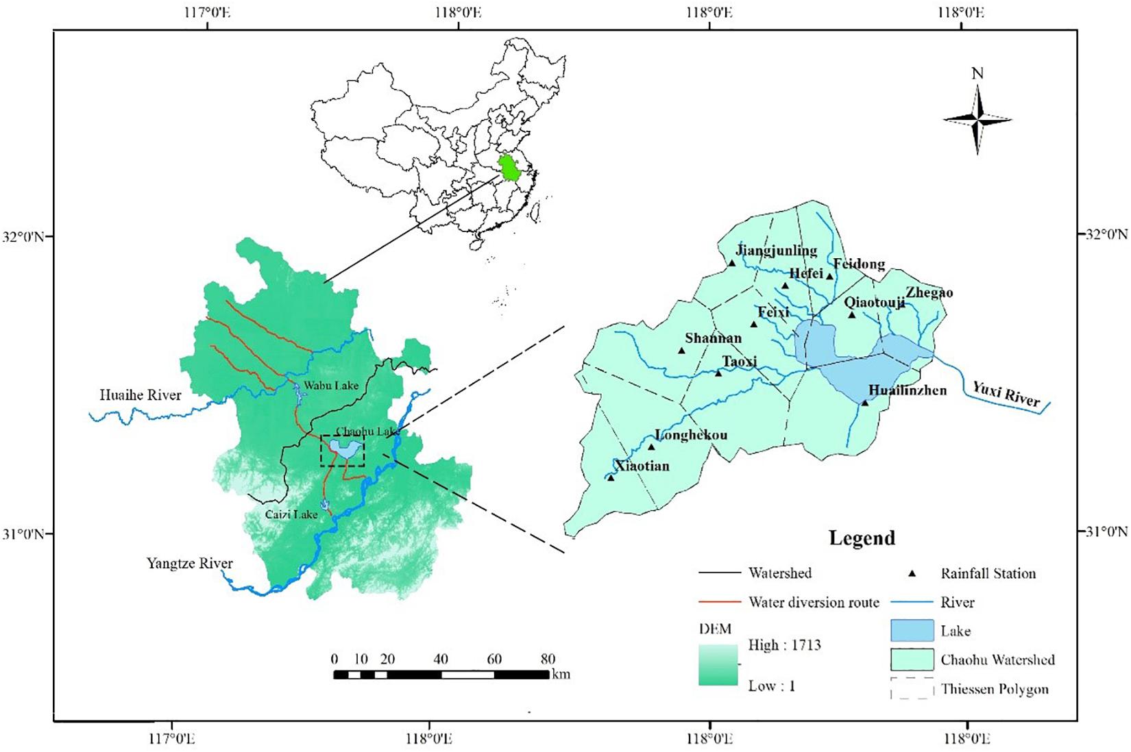
Figure 1. Location map for study and gauge stations.

The climate is northern subtropical and warm temperate humid monsoon climate, which is characterized by a mild climate, significant monsoon rainfall, a well-defined rainy season, good heat conditions, and a long frost-free season. The average annual precipitation (AP) is about 1095 mm. The spatial distribution of precipitation in the basin is uneven, decreasing from south to north. Meanwhile, precipitation is unevenly distributed during the year, and more than 60% of the annual total precipitation occurs in the period from June to September. The average annual temperature and evaporation are about 16.5°C and 880 mm, respectively.

Data from a total of 11 meteorological stations covering the approximate period of 1958∼2017 were collected, and these were retrieved from the Anhui Provincial Bureau of Hydrology. Meanwhile, basin areal precipitation and evaporation were calculated by the Thiessen polygons method. The annual highest water level (AHWL) data were collected from Zhongmiao hydrological gauging station, which is situated at the center of Chaohu Lake.

Methodology

To understand the characteristic of daily lake inflows in typical hydrological years, this research is divided into four subsections that describe the main components, including the following: (1) determination of typical hydrological years based on the bivariate frequency analysis of AP and AHWL; (2) calculation of the Chaohu Lake inflows of selected flood events depends on water balance method; (3) determination of the optimal parameters of the coupled model predictions by I-SOPSO method; and (4) generation of long-series inflow simulate results on the basis of model optimal parameters. The details of the evaluation procedures of the above methods are discussed in the following subsections.

Hydrologic Frequency Analysis

In the actual hydrological design, several typical years are selected from the hydrological data for analysis and calculation, and the results can generally meet the requirements of planning and design. Hydrological frequency analysis is usually a more powerful tool for selecting typical years. Generally, application of the bivariate probability analysis allows researchers to investigate hydrological events with a more comprehensive view by considering the simultaneous effect of the influencing factors on the phenomenon of interest (Yue et al., 1999; Vandenberghe et al., 2011; Sraj et al., 2015). Therefore, a two-dimensional joint theoretical cumulative distribution function of AP and AHWL was constructed, and the specific process can refer to the following steps.

Step 1 Marginal Cumulative Distribution Function of AP and AHWL

Pearson-III distribution function (P-III), which can be described with three parameters, mean value ($\overline{x}$), variation coefficient (_cv), and skew coefficient (_cs) of the observation data, was considered as marginal distribution functions (MDF) of AP and AHWL. The calculation formula of the cumulative probability includes α, β, and a₀, which are the parameters of shape, scale, and location (Lei et al., 2018). The probability density function and the cumulative frequency equation (cumulative frequency greater than or equal to x_p) are shown in formulas 2 and 3:

$$\mathrm{\alpha }=\frac{4}{C_s^2}\mathit{\hspace{1em}\hspace{0.5em} }\mathrm{\beta }=\frac{2}{\overline{x}{C}_v{C}_s}\mathit{\hspace{1em}\hspace{0.5em} }{a}_0=\overline{x}(1-\frac{2C_v}{C_s})(1)$$

$$f(x)=\frac{{\mathrm{\beta }}^{\mathrm{\alpha }}}{\mathrm{\Gamma }(\mathrm{\alpha })}{(x-a_0)}^{\mathrm{\alpha }-1}{e}^{-\mathrm{\beta }(x-a_0)}(2)$$

$$P=P(x\ge x_p)=\frac{{\mathrm{\beta }}^{\mathrm{\alpha }}}{\mathrm{\Gamma }(\mathrm{\alpha })}{\int }_{x_p}^{\mathrm{\infty }}{(x-a_0)}^{\mathrm{\alpha }-1}{e}^{-\mathrm{\beta }(x-a_0)}(3)$$

Step 2 Investigation of Correlation Between Variables

In the copula approach, the dependence between the pairs of considered variables should be analyzed. Kendall’s correction coefficient, which is widely used because Kendall’s tau (τ) is more insensitive to ties in data, was selected and calculated by the Eq. 1:

$$\mathrm{\tau }={(C_n^2)}^{-1}\sum _{i\mathrm{?}j}sign[x_i-x_j)(y_i-y_j)](4)$$

where n is the number of variable data pairs (x_i, y_i). In addition, sign(.) is a symbolic function, which is defined as follows:

$$sign=\{\begin{array}{c}1\mathit{\hspace{1em}\hspace{1em}\hspace{1em}\hspace{1em}\hspace{1em}}(x_i-x_j)(y_i-y_j)>0\hfill \\ -1\mathit{\hspace{1em}\hspace{1em}\hspace{1em}\hspace{0.5em}\hspace{1em}}(x_i-x_j)(y_i-y_j)<0\hfill \\ 0\mathit{\hspace{1em}\hspace{1em}\hspace{1em}\hspace{1em}\hspace{1em}}(x_i-x_j)(y_i-y_j)=0\hfill \end{array}(5)$$

where x_i and y_i are observed data corresponding to random variables X and Y in the ith year.

Step 3 Construction of Copula Function

Generally, the copula function can be classified into three types, i.e., copulas with a quadratic form, copulas with a cubic form, and Archimedean copulas. Among them, the Archimedean copulas, the one-parameter bivariate copulas, are found to be more desirable for hydrologic analysis (Genestm and Mackaym, 1986). Meanwhile, Clayton, Frank, and Gumbel–Hougaard’s copula functions were adopted because the proper copulas directly depend on the value of Kendall’s tau (τ) (Ahmadi et al., 2018):

(A) Clayton Copula

$$C_{\mathrm{\theta }}[x,y]={[x^{-\mathrm{\theta }}+y^{-\mathrm{\theta }}-1]}^{-1/\mathrm{\theta }}\mathit{\hspace{1em}\hspace{1em}}\mathrm{\theta }=\frac{\mathrm{\tau }}{1-\mathrm{\tau }}\mathit{\hspace{1em}\hspace{1em}}\mathrm{\theta }\in (0,\mathrm{\infty })(6)$$

(B) Gumbel–Hougaard Copula

$$C_{\mathrm{\theta }}[x,y]=\exp \{-{[-{(\ln x)}^{\mathrm{\theta }}+{(-\ln y)}^{\mathrm{\theta }}]}^{1/\mathrm{\theta }}]\}\mathrm{\theta }=\frac{1}{1-\mathrm{\tau }}\mathrm{\theta }\in [-1,\mathrm{\infty })(7)$$

(C) Frank Copula

$$\begin{array}{c}\hfill C_{\mathrm{\theta }}[x,y]=-\frac{1}{\mathrm{\theta }}\left[1+\frac{\left[\exp (-\mathrm{\theta }x)-1\right]\left[\exp (-\mathrm{\theta }y)-1\right]}{\exp (-\mathrm{\theta })-1}\right]\hfill \\ \hfill \mathrm{\tau }=(\frac{3\mathrm{\theta }-2}{\mathrm{\theta }})-\frac{2}{3}{(1-\frac{1}{\mathrm{\theta }})}^2\ln (1-\mathrm{\theta })\mathit{\hspace{1em}\hspace{1em} }\mathrm{\theta }\in R\hfill \end{array}(8)$$

where parameter θ describes the relationship between the two random variables X and Y.

Step 4 Selection of the Best-Fit of Copula

The limitation of the copula approach is that there are no specific ways to check whether the dependency structure of a data set is appropriately modeled by the chosen copula (Dodangeh et al., 2019). In this part, three commonly used methods, including the graphic analysis, Kolmogorov–Smirnov, and Akaike Information Criterion (AIC), were applied to select the best suitable copula function for Chaohu Lake Watershed.

(A) Graphic analysis

The graphic analysis method is a method that uses a graph to intuitively represent the effect of a theoretical probability distribution on the measured value. In this graphic, bivariate joint empirical cumulative frequency (BJECF) is often calculated to compare with the copula theoretical curves (Sraj et al., 2015). The BJECF can be estimated using the approach of Yue et al. (1999):

$$F_o(x_i,y_i)=P(X\le x_i,Y\le y_j)=\frac{{\sum }_{m=1}^i{\sum }_{l=1}^j{n}_{ml}-0.44}{n+0.12}(9)$$

(B) Kolmogorov–Smirnov

$$D_n=\underset{1\le i\le n}{\max }[\left|\frac{m(i)-1}{n}-F_c(x_i,y_i)\right|,\left|F_c(x_i,y_i)-\frac{m(i)}{n}\right|](10)$$

(C) Akaike Information Criterion (AIC)

$$\begin{array}{c}\hfill AIC=n\ln (MSE)+2m\hfill \\ \hfill MSE=\frac{1}{n}\sum _{i=1}^n{[P_c(i)-P_o(i)]}^2\hfill \end{array}(11)$$

where, n is the number of variable data pairs (x_i, y_i); n_ml is the number of joint observation sample satisfying two conditions at the same time: x_m ≤ x_i and y_l ≤ y_j, which have the same meanings as m(i) in this paper. F_c(x_i,y_i) and F_o(x_i, y_i) are the cumulative joint theoretical probability and experience frequency distribution function, respectively; P_o(i) is the ith year observed value obtained from cumulative joint empirical frequency function; P_c(i) is the calculated value of the ith year of by the bivariate copula function; and m is the number of model parameters. Moreover, the smaller the values of D_n and AIC are, the better the simulation results are.

Water Balance Method

For a given lake basin, the water balance equation is as follows:

$$P+R_a+R_g=E+R_a^{\prime }+R_g^{\prime }+u+\mathrm{\Delta }S(12)$$

where P is the precipitation on the lake during the period; R_a, R’_a are the surface runoff into and out of the lake during the period; R_g, R’_g are the underground runoff into and out of the lake during the period; E is the effective evaporation during the period; μ represents the consumption of industrial and agricultural; and ΔS indicates the change of water storage within a period of time. The above units are all in m³.

Hydrologic Model

The input data of the Xin’anjiang model includes precipitation (P) and pan evaporation (EM), while the output of the module the is discharge of the outlet (Q_m). There are 15 parameters (outside the box in Figure 2) involved in the model for flow routing, which could be grouped as Supplementary Table 1. In principle, these parameters are spatially uniform, meaning that they represent integrated effects of catchment properties. More details about the calculation of the Xin’anjiang model can be found in Zhao (1992).

FIGURE 2

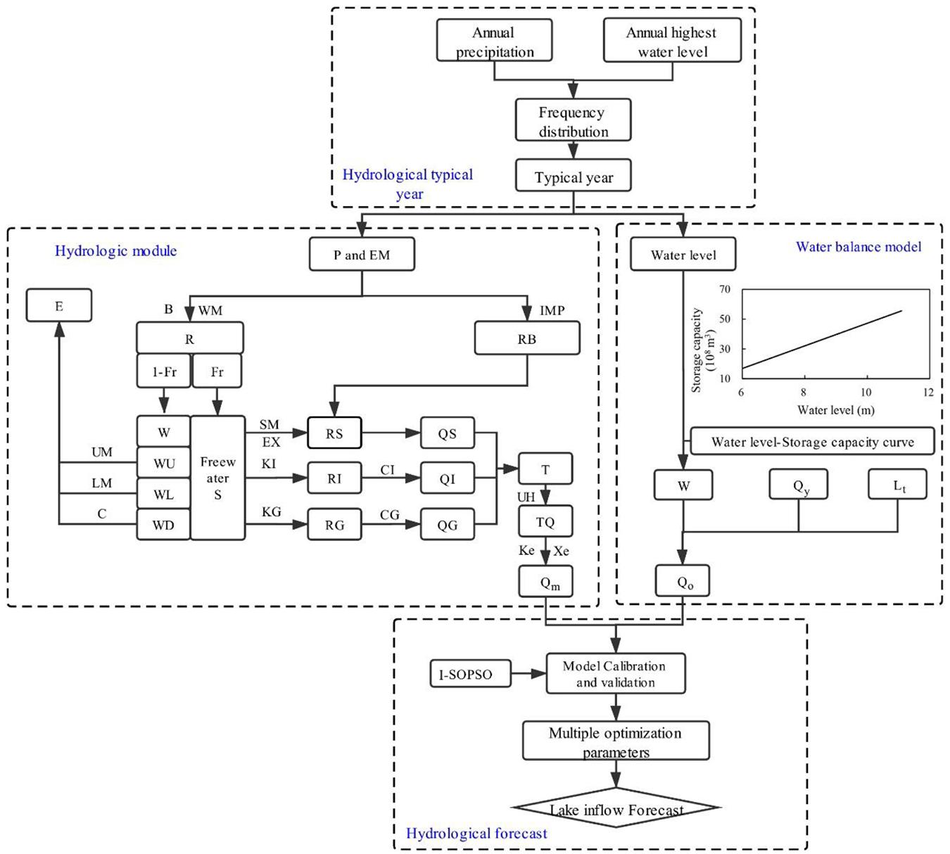
Figure 2. Technique path map of the research. Fr: contribution area; RB: runoff of impervious area; S: free water; QS: total surface runoff; QI: total interflow; QG: total groundwater runoff; Other parameter meanings can be seen in Supplementary Table 1.

Model Calibration

In a hydrologic model, some model parameters cannot be directly obtained from the basin characteristics using existing measured streamflow data in the field. It is common that a set of accurate model parameters are determined by fitting the observation data and simulation values that are calculated by adjusting the model parameters, which is called the calibration of the model. In order to find the optimal parameters of the model, the SOPSO method, which is a population-based optimization technique proposed in 1995 (Eberhart and Kennedy, 1995), was added to the Xin’anjiang model to simulate the Lake inflows. However, the SOPSO method may not be able to directly calibrate the model given the limitations of the actual inflow data (intermittent flood events) calculated by water balance. Therefore, the I-SOPSO method is applied to the Xin’anjiang model, and three things need to be done during the running of the model: (1) reading the input daily precipitation and evaporation data in sequence; (2) the daily inflow data of selected flood events are used to calibrate the parameters of the model; and (3) using the optimized parameters to calculate the long series of daily lake inflows.

More details on the calculation process of the SOPSO can be found in the literature (Kamali et al., 2013). The maximum WANSE of selected flood events is used as the objective function to minimize the error in estimating the goodness-of-fit between observed and simulated values shown in Eq. (13) below:

$$WANSE=\frac{1}{N}\left(\sum _{i=1}^N{\mathrm{\omega }}_i\times (1-\frac{{\sum }_{t=1}^T{(Q_{oi}^t-Q_{mi}^t)}^2}{{\sum }_{t=1}^T{(Q_{oi}^t-{\overline{Q}}_{oi})}^2})\right)(13)$$

where N is the total number of calibration flood events; ω_i shows the degree of important given to ith flood event; ${\overline{Q}}_{oi}$ is the mean of observed inflows of ith flood event; $Q_{mi}^t$ and $Q_{oi}^t$ are the modeled and observed inflows of ith flood at time t; and T is the final time step. The WANSE value is selected because it is more sensitive to peak flows, and approximate values close to 1 indicate better performances.

Model Performance Assessment

The flood peak, volume, and hydrograph shape are three basic elements describing a flood event (Yue et al., 1999). In this study, the following commonly used five statistical indicators, including the water balance index (WBI) (Deng et al., 2015), Nash-Sutcliffe efficiency (NSE), percent error in peak flow (F_peak), flood volume estimation error (F_vol), and determination coefficient (R²), were adopted to further evaluate the performance of the coupled model, which can provide a quantitative and aggregate estimate of model reliability as follows:

$$WBI(\%)=\frac{\mathrm{\Delta }V-(W_I-W_O)}{\mathrm{\Delta }V}\times 100(14)$$

$$NSE=1-\frac{{\sum }_{t=1}^T{(Q_o^t-Q_m^t)}^2}{\sqrt{{\sum }_{t=1}^T{(Q_o^t-\overline{Q}{}_o)}^2}}(15)$$

$$F_{peak}(\%)=\frac{Q_o^{peak}-Q_m^{peak}}{Q_o^{peak}}\times 100(16)$$

$$F_{vol}(\%)=\frac{Vo{l}_o-Vo{l}_m}{Vo{l}_o}\times 100(17)$$

$$R^2=\frac{{\sum }_{t=1}^T(Q_m^t-\overline{Q}{}_m)(Q_o^t-\overline{Q}{}_o)}{\sqrt{{\sum }_{t=1}^T{(Q_m^t-\overline{Q}{}_m)}^2{(Q_o^t-\overline{Q}{}_o)}^2}}(18)$$

W_I and W_O are the total volumes of lake inflow and release calculated by water balance method (10⁸ m³) in which the time step to be considered is 1 day; ΔV is lake storage change, which represents the difference between the initial and final lake storages during a flood event; $Q_o^{peak}$ and $Q_m^{peak}$ designate as peak flows of observed and simulated hydrographs (m³/s); $Q_o^t$, $Q_m^t$, $\overline{Q}{}_m$, and $\overline{Q}{}_o$ are the observed and simulated lake inflow at time t, mean of observed and simulated lake inflows (m³/s), respectively; and Vol_o and Vol_m are the observed and the simulated total volume during a flood event (10⁸ m³). The standard error range of the WBI index refers to the allowable error of flood volume (runoff depth) of reservoir hydrological simulate.

Results and Discussion

Selection of Typical Hydrological Year

Marginal Cumulative Probability Distribution Analysis

Before performing frequency analysis, the data homogeneity of AP and the annual maximum water level series have been tested.

Probability analysis of annual precipitation

As we all know, natural runoff is the basis of hydrological analysis. However, natural streamflow observations are not always available in many parts of the world, especially in Lake Basins that have multiple tributaries, see the impact of anthropogenic activities, and do not have observation data. Therefore, in actual research, many scholars use precipitation data that is less affected by anthropogenic activities to carry out the hydrological frequency analysis and obtain very good results (Vandenberghe et al., 2011; Dodangeh et al., 2019).

In this paper, the results of AP frequency analysis indicate that the fitted distribution curve performs well (fitting degree = 0.983) due to good agreement between observed AP data and theoretical probability (Figure 3A). The 60-year AP series has an average ($\overline{x}$) of 1094.67 mm, a deviation coefficient (c_v) of 0.19, and a skewness (c_s) of 0.34. Meanwhile, box-whisker plots of absolute error of AP frequency show that the maximum and minimum relative errors are 4.18 and −5.3% (Figure 3C), which occurred in 1961 and 1974, respectively.

FIGURE 3

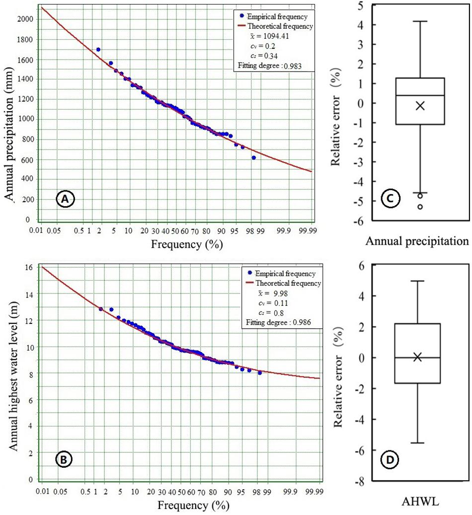
Figure 3. Probability of univariate empirical scatter plots and fitted theoretical probability curve (A: Annual precipitation; B: Annual maximum water level) and the relative error between empirical frequency and theoretical frequency (C: Annual precipitation; D: Annual maximum water level).

Probability analysis of annual highest water level

The amount of lake inflow will directly reflect the water level change of the lake. At the same time, considering the availability of data and the hydrological situation of the whole study area, the AHWL of the lake is also a useful index for frequency analysis. In this study, the AHWL data of the Zhongmiao station is used for frequency analysis (Figure 3B). Figure 3B shows the fitting curve followed the observed dataset reasonably well. The probability distributions of calibrated parameter values can be estimated roughly by Figure 3B, which are 10.06 m ($\overline{x}$), 0.11 (c_v), and 0.8 (c_s), respectively. The distribution of relative error ranges from −5.53 to 4.97% (Figure 3D), with an average value of 0.04%. Consequently, the P-III fitting curve is reasonable as the marginal cumulative probability distribution function.

In Supplemental Information (Part A), details can be found on the comparison probability analysis of AP and AHWL.

Bivariate AP-AHWL Probability Analysis

There is a causal relationship between the change of lake level and precipitation. Meanwhile, from a statistical perspective, the correlation coefficient between the AP and the AHWL is 0.82 (Figure 4A), which belongs to highly correlated. The correlation coefficient between the AP (11 rainfall stations) and AHWL is between 0.66 and 0.82, Figure 4B respectively. Therefore, the two variables (AP and AHWL) are considered at the same time to selected the typical years in the study.

FIGURE 4

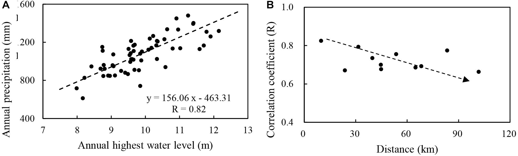
Figure 4. Variable relationship analysis (A) AP versus AHWL and (B) the correlation coefficient between AHWL and AP of 11 rainfall stations versus vertical distance from Zhongmiao hydrological station.

The theoretical joint probability distribution of the 60-year historical hydrological series results of the three copula functions are presented in Figure 5. Based on the graphic analysis method (Figures 5A,B), the Gumbel–Hougaard function best represents the bivariate distribution of the AP and AHWL during almost the entire year, followed by the Clayton function, with the Frank function being the worst. Meanwhile, the order of AIC values from small (good) to large (bad) is −433.8 (Gumbel–Hougaard method), −405.2 (Clayton method), and −299 (Frank method), which is in agreement with the finding of the graphic analysis method, as, the smaller the value is, the better the fitting degree is. What is more, in the Kolmogorov–Smirnov test, the p-values of the three copula functions are greater than 0.05, indicating that there is no significant difference from the empirical frequency, while the D_n values of Clayton method (0.08), Gumbel–Hougaard method (0.1), and Frank method (0.15) indicate that Clayton Copula function has the best fit. Thus, considering the fit of the whole series, the Gumbel–Hougaard copula function was chosen to select the typical hydrological years, which are 1978, 2007, and 2016 (Table 1).

FIGURE 5

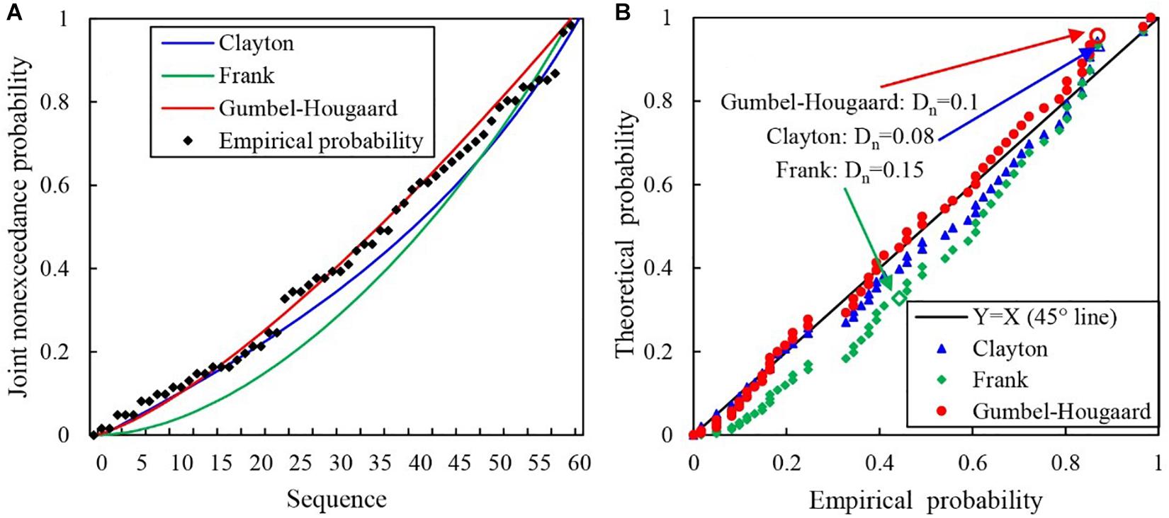
Figure 5. Comparison of joint cumulative probability distributions obtained using three copula methods with empirical probability.

TABLE 1

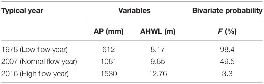
Table 1. Characteristic statistics of typical years.

Results of Water Balance Method

The lake/reservoir inflow observation records are important for hydrological research and practice projects, such as flood simulations, hydraulic engineering design, water resource planning and management, etc. (Zhou et al., 2019). Because detailed and accurate daily data are difficult to obtain (Deng et al., 2015), a water balance analysis was only applied to calculate the daily inflow of flood events.

Before taking the inflow calculated by water balance as the measured runoff, it is necessary to verify whether the measured daily inflow (land runoff) calculated by the water balance method is reasonable. In this part, the change in the lake storage of a flood can be obtained in two ways: (1) changes in storage capacity corresponding to the beginning and final time of each flood event named ΔV; and (2) changes in the total runoff obtained by daily observed inflow which calculated by water balance method, namely, W_I-W_O. The WBI index is used to evaluate the water balance method performance for the study area during flood events. It can be seen from Table 2 that the order of the overall calculation errors (from small to large) for the three typical years is as follows: 2007, 2016, and 1978. The WBI values of 12 flood events are between 1.4 and −19.5%, which is within the standard error range (±20%). The values of WBI of the selected flood events are positive/negative, indicating that using the water balance method would overestimate/underestimate the lake flows, which may be caused by missing data for actual scheduling rules of Chaohu sluice and Zhaohe sluice, the imprecise relationship between water level and lake storage that is obtained by linear fitting of measured discrete points. Although there are many factors that affect the accuracy of the calculation, the calculated results show that the method can be applied to calculate the daily lake inflows during the flood period.

TABLE 2

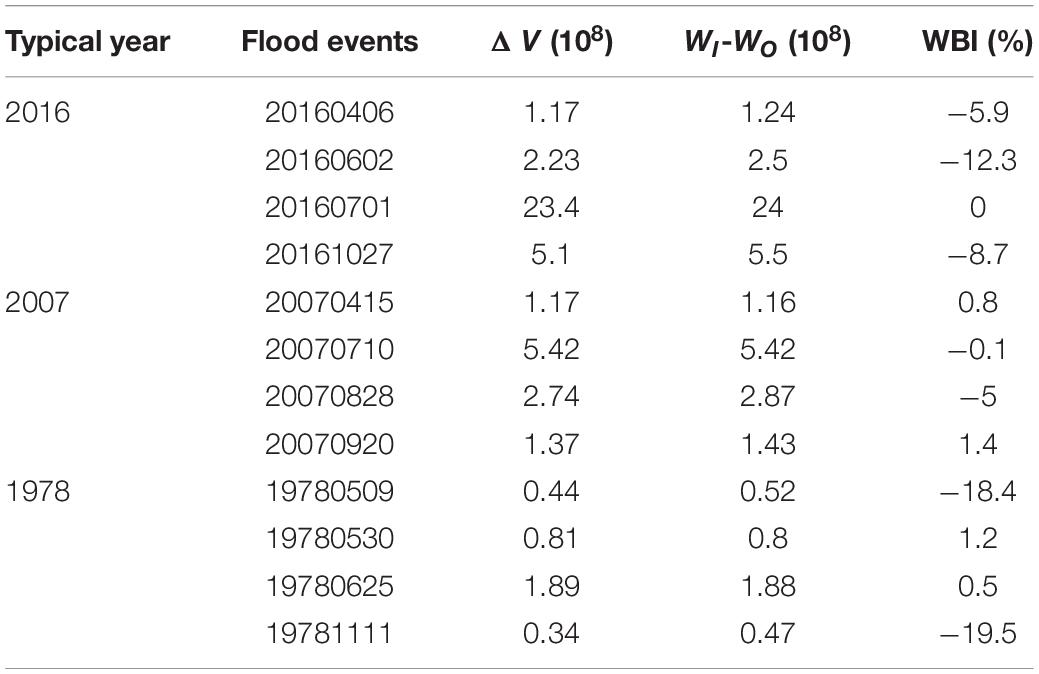
Table 2. Performance of water balance during flood events.

Calibration and Validation of the Coupled Model

High Flow Year

The I-SOPSO algorithm is linked to the coupled model in a Fortran environment, and the I-SOPSO maximizes the calibration objective function, which is the sum of weighted NSE calculated by comparing observed (calculated by water balance method) and simulated hydrograph. Four flood events were selected at daily time steps in 2016–the April 6, July 1, and October 27 flood events are the calibration period and the June 2 flood event the validation period–considering the short time interval between the June 2 and July 1 flood events. The NSE, F_peak, F_vol, and R² were calculated to evaluate the performance of the coupled model, as shown in Table 3 and Figure 6.

TABLE 3

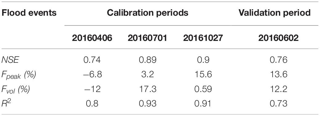
Table 3. Simulation performances of hydrograph of selected flood events in high inflow year by the coupled water balance method and Xin’anjiang model.

FIGURE 6

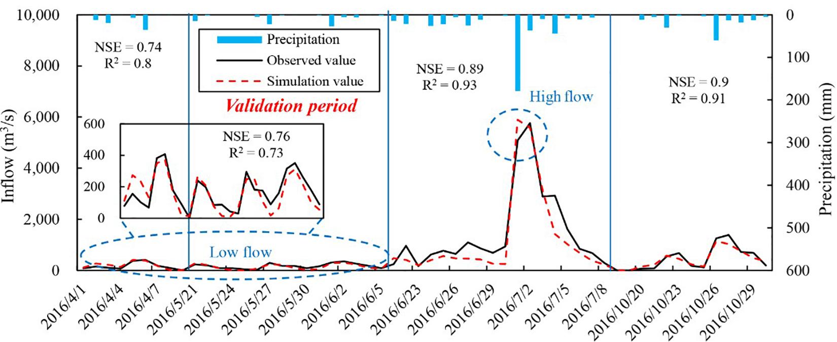
Figure 6. Results for the four flood events of Lake inflows.

For the graphic evaluation of the model, the daily inflow of the four flood events observed were well followed by the simulated runoff from the coupled model. In Table 3, the values of NSE are 0.74, 0.89, and 0.9 during the calibration periods, and, for the validation period, the value of NSE is 0.76, indicating that the coupled water balance and the Xin’anjiang model can reasonably predict the general shapes of the hydrographs (Figure 6). In terms of R², which is the linear correlation between and simulated results and observed data, the R² values of four flood events are more than 0.73, with a mean of 0.85, which is an acceptable statistic that confirms the capability of the model simulate the catchment response (Mahmood and Jia, 2019). The total runoff volume errors (F_vol) and the peak inflow estimation errors (F_peak) are within 20% of the four flood events on a daily scale, which meet the level standard required for flood simulation (MWR, 2008). Considering the results of four evaluating indicators, the coupled model can obtain desirable results in a study area, which provides technical support, especially in the practical application process to solve the lack of data or incomplete data lake or reservoir basin.

The values of F_peak are −6.8, 13.6, 3.2, and 15.6%, with relatively large errors, which may be induced by the error from water level observation. For example, when the water level in Chaohu Lake is 8.0 m (normal storage level) and its observation error is 0.1 m, the induced error of reservoir storage volume and estimated daily inflow are about 0.77 × 10⁸ m³ and 885.4 m³/s, respectively. The calculation of the objective function of the model may be another uncertainty source (Tian et al., 2014). In the calculation of the model, the July 1, 2016, flood event was considered with a larger weight (three times that of other flood events), taking into account the greater hazards based on the flood peak and flood volume. The advantage of using different weights can avoid fall into a situation of overfitting in a certain flood but neglecting the important flood events.

For F_vol, the value of the July 1, 2016, flood event (17.3%) is slightly larger than the other flood events, which is seriously under-estimated the total volume of lake inflow. There are many reasons for the deviation of model calculation results.

Precipitation is a key component to drive the hydrologic model. The heterogeneous spatial and temporal distributions in basins, inadequate precipitation stations, and location of the rainfall center may normally influence the quality of simulate accuracy (Xu et al., 2013; Zeng et al., 2018; Zhong et al., 2018). During the study period, the July 1, 2016, flood event is characterized by a long-term rainstorm and the uneven spatial distribution of precipitation. In order to understand the spatial distribution of precipitation in the third (July 1, 2016) flood event in detail, 33 rainfall stations in the Yearbook were collected to make the spatial distribution map. It can be seen that the highest values of P are related to the south part of the Chaohu Lake (278.3, 410.8, 516.2, and 646.9 mm), while the northern part shows the lowest level of P for the total maximum precipitation in 1-day, 3-day, 5-day or total precipitation volume (51.8, 76.3, 91, and 187.1 mm, respectively) during the July 1, 2016, flood event (Figure 7). The total area precipitation based on the Thiessen polygons method in the model is 424 mm during the July 1, 2016 flood event, which lacks the flexibility to investigate possible spatial evolution of model parameters. Heterogeneous spatial precipitation, as a fundamental process of hydrological cycle, is the first major source of uncertainty in the results of the present study.

FIGURE 7

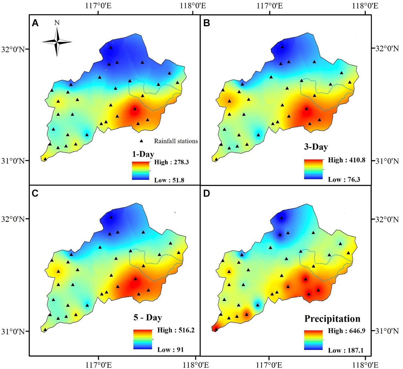
Figure 7. Spatial distributions of total maximum precipitation in 1-day (A), 3-day (B), 5-day (C), or total precipitation volumes (D) in the July 1, 2016 flood event (Units: mm).

Meanwhile, the storage of small reservoirs and the regulation of sluices and dams are not considered in the model structure, which will cause deviations in the calculation results of the inflow process and flood inflow, e.g., Longhekou reservoir, located in Hangbu River, which is the biggest reservoir with a drainage area of 1120 km², and the inflow to the reservoir is mainly the result of localized rainfall. According to the yearbook, the maximum daily flow of Longhekou Reservoir Station was 805 m³/s, according to the data, there is no discharge, and there should be no discharge based on the control operation rules. However, the actual release of reservoirs release is unclear in this study. In addition, the model’s structure is probably another reason because the Xin’anjiang model was built for the regions either low or high surface runoff with the assumption that surface runoff is not generated until the soil moisture content reaches field capacity, but in some cases, like in the mountainous areas and cities, the flood could happen when the intensity of rainfall is large without filling up the soil storage. Therefore, limited and understanding of nature and simplifications in representing the hydrological processes, Xin’anjiang model structures must be in error to some extent, although the structure and parameters of the model can reflect the main laws and characteristics of rainfall and runoff process in humid areas and can obtain better precision.

Besides, most parameters of the model cannot be measured via direct observations in the field but through practice to estimate parameter values with historical observation data using an improved automated search algorithm (I-SOPSO). In this process, the system identification method is used to optimize the debugging, so the variables and parameters in existing hydrology models determined may not be the optimal results (Wu et al., 2017; Mahmood and Jia, 2019). These different sources of uncertainty act to compound the rainfall-runoff simulating and can have a significant impact on the accuracy of simulation results. However, if we assumed that the abovementioned uncertainties can affect the result of the present study by 15∼20% (Coe and Foley, 2001), the results of the present study are still quite satisfactory and can be a good source for understanding the lake inflow process.

Low Flow Year and Normal Flow Year

The performance of selected flood events in the normal flow year and the low flow year is summarized in Table 4. It can be seen from this table that there are three and five calculated index values exceeding the critical values for the normal flow year and the low flow year. Considering the comprehensive level of the four indicators, the simulation results of in the normal flow year (2007) are better than in the low flow year (1978) and worse than in the high flow year (2016), indicating that there is a more complex relationship between rainfall and runoff due to the intervention of more anthropogenic activities and climate change. As one of the primary farming areas of China, the landscape of the Chaohu Lake Basin consists mainly of farmland, woodland area, and water body accounting for 61.8, 16, and 10.3%, respectively. Meanwhile, surface water bodies (rivers and lake) in the study area are important water resources for local agriculture activities.

TABLE 4

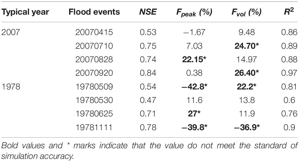
Table 4. Summary of performance of selected flood events in 2007 and 1978 year.

For better understanding and water resources planning and management, it is suggested to take into account and reduce sources of uncertainty when making hydrological simulate. In the present study, quantifying and reducing uncertainty in hydrological modeling from multiple sources, i.e., parameter uncertainty, input uncertainty, and model structural uncertainty, are not included in this study considering that the current calculation results meet the requirements. Further research can be carried out to improve the accuracy of the model through more accurate input data sets and uncertainty analysis.

Long-Series of Lake Inflow Simulation

According to the optimal parameters of the calibrated coupled model, the daily runoff hydrograph is simulated (Figure 8). According to the previous investigation project, the entire Chaohu Lake Basin with an area of 13486 km² (including the surface area of Chaohu Lake) has an average runoff of 34.9 × 10⁸ m³. Meanwhile, the surface runoff of Chaohu Lake is 6.3 × 10⁸ m³, which is calculated by multiplying the lake area with the annual mean net precipitation. Therefore, the average land surface runoff of the study area, which is calculated by weighting the land surface catchment area (weight = 0.66), is 18.9 × 10⁸ m³. The result of the annual inflow (land runoff) of the study area was calculated by the coupled model to be 19.4 × 10⁸ m³ in the normal flow year, and the corresponding bivariate probability is 49.5%. The relative error is −2.6%, indicating that the coupled water balance and Xin’anjiang model are available in the study area, which can better simulate the daily inflow process of the lake without the measured runoff data. The calculated land inflows of the high flow and the low flow years are 44.4 × 10⁸ m³/a and 13.7 × 10⁸ m³/a, respectively.

FIGURE 8

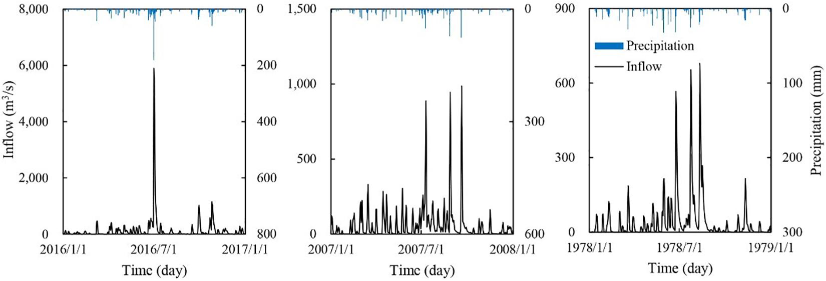
Figure 8. Daily lake inflow hydrograph of the typical years.

Conclusion

In this paper, the copula functions are adopted to establish the bivariate probabilistic model for simulating the AP and AHWL between 1956 and 2017. The coupled water balance method and Xin’anjiang model is then used to explore lake inflows of Upper Chaohu Lake Watershed to gather more information.

The goodness-of-fit test indicates that the Gumbel–Hougaard function is the best-fit for AP-AHWL with Pearson-III margin distributions, which is thereby applied to select the typical hydrological year, including high flow (2016), low flow (1978), and normal flow years (2007). Furthermore, the WBI values of the flood events are within 20%. Overall, the order of the WBI values (from small to large) for the three typical years is 2007, 2016, and 1978. The calibration and verification results of the coupled water balance method and the Xin’anjiang model show that the simulated results are better in the high flow year than in the normal flow and low inflow year. Some calculated index values exceed the critical values for normal inflow year and low inflow year, which is most probably caused by the parameter uncertainty, input uncertainty, and model structural uncertainty. Finally, the result of comparison the annual lake inflow simulation in normal inflow year (19.4 × 10⁸ m³) and the results of the average land surface runoff of the study area (18.9 × 10⁸ m³) indicates that the coupled Xin’anjiang model and water balance method are effective ways to calculate the daily lake inflow. The land inflows in high flow year and low flow year are 44.4 × 10⁸ m³ and 13.7 × 10⁸ m³, respectively. In conclusion, the results of this paper are helpful to understand the daily lake inflows process in Upper Chaohu Lake Basin. They can be used as a basis for determining the appropriate operation and management of water resource systems.

Data Availability Statement

All data, models, or code generated or used during the study are available from the corresponding author by request (behellen@163.com).

Author Contributions

XL provided the technical guidance. WL provided the manuscript ideas and financial support. QY mainly revised the language issues of the manuscript. SC provided basic data. XW gave amendments to the details of the manuscript. JW and CW were in the process of calculation some constructive suggestions were given. ZL organized the overall calculation, writing and drawing of the manuscript. All authors contributed to the article and approved the submitted version.

Funding

This manuscript was jointly supported by Young Elite Scientists Sponsorship Program by CAST (2019QNRC001), the National Key R&D Program of China (2017YFC0406004), the National Natural Science Fund (51709273), and the Key R&D Program of Power Construction Corporation of China (DJ-ZDZX-2016-02).

Conflict of Interest

The authors declare that the research was conducted in the absence of any commercial or financial relationships that could be construed as a potential conflict of interest. The reviewer JZ declared a past co-publication with the authors XL and WL. The reviewer CM declared a past co-publication with the authors XL and WL.

Supplementary Material

The Supplementary Material for this article can be found online at: https://www.frontiersin.org/articles/10.3389/feart.2021.615692/full#supplementary-material

References

Ahmadi, F., Radmaneh, F., Sharifi, M. R., and Mirabbasi, R. (2018). Bivariate frequency analysis of low flow using copula functions (case study: Dez River Basin, Iran). Environ. Earth Sci. 77:643. doi: 10.1007/s12665-018-7819-2

CrossRef Full Text | Google Scholar

Bai, P., Liu, X., Liang, K., Liu, X., and Liu, C. (2017). A comparison of simple and complex versions of the Xinanjiang hydrological model in predicting runoff in ungauged basins. Hydrol. Res. 48, 1282–1295. doi: 10.2166/nh.2016.094

CrossRef Full Text | Google Scholar

Cao, Z., Li, S., Zhao, Y., Wang, T., Bergquist, R., Huang, Y., et al. (2018). Spatio-temporal pattern of schistosomiasis in Anhui Province, East China: potential effect of the Yangtze River - Huaihe River Water Transfer Project. Parasitol. Int. 67, 538–546. doi: 10.1016/j.parint.2018.05.007

PubMed Abstract | CrossRef Full Text | Google Scholar

Coe, M. T., and Foley, J. A. (2001). Human and natural impacts on the water resources of the Lake Chad basin. J. Geophys. Res. Atmospheres 106, 3349–3356. doi: 10.1029/2000JD900587

CrossRef Full Text | Google Scholar

Deng, C., Liu, P., Liu, Y., Wu, Z., and Wang, D. (2015). Integrated hydrologic and reservoir routing model for real-time water level forecasts. J. Hydrol. Eng. 9:05014032. doi: 10.1061/(asce)he.1943-5584.0001138

PubMed Abstract | CrossRef Full Text | Google Scholar

Dodangeh, E., Shahedi, K., Solaimani, K., Shiau, J., and Abraham, J. (2019). Data-based bivariate uncertainty assessment of extreme rainfall-runoff using copulas: comparison between annual maximum series (AMS) and peaks over threshold (POT). Environ. Monit. Assess. 191:67. doi: 10.1007/s10661-019-7202-0

PubMed Abstract | CrossRef Full Text | Google Scholar

Eberhart, R., and Kennedy, J. (1995). “A new optimizer using particle swarm theory,” in Proceedings of the 6th International Symposium on Micro Machine and Human Science MHS’95, Nagoya, 39–43.

Google Scholar

Gal, L., Grippa, M., Hiernaux, P., Peugeot, C., Mougin, E., and Kergoat, L. (2016). Changes in lakes water volume and runoff over ungauged Sahelian watersheds. J. Hydrol. 540, 1176–1188. doi: 10.1016/j.jhydrol.2016.07.035

CrossRef Full Text | Google Scholar

Genestm, C., and Mackaym, J. (1986). The joy of copulas: bivariate distributions with uniform marginals. Am. Stat. 40, 280–283. doi: 10.2307/2684602

CrossRef Full Text | Google Scholar

Kamali, B., Mousavi, S. J., and Abbaspour, K. C. (2013). Automatic calibration of HEC-HMS using single-objective and multi-objective PSO algorithms. Hydrol. Process. 27, 4028–4042. doi: 10.1002/hyp.9510

CrossRef Full Text | Google Scholar

Lei, G., Yin, J., Wang, W., and Wang, H. (2018). The analysis and improvement of the fuzzy weighted optimum curve-fitting method of pearson – type III distribution. Water Resour. Manag. 32, 4511–4526. doi: 10.1007/s11269-018-2055-9

CrossRef Full Text | Google Scholar

Li, Y., Cui, Q., Li, C., Wang, X., Cai, Y., Cui, G., et al. (2017). An improved multi-objective optimization model for supporting reservoir operation of China’s South-to-North Water Diversion Project. Sci. Total Environ. 575, 970–981. doi: 10.1016/j.scitotenv.2016.09.165

PubMed Abstract | CrossRef Full Text | Google Scholar

Lin, K., Lv, F., Chen, L., Singh, V. P., Zhang, Q., and Chen, X. (2014). Xinanjiang model combined with Curve Number to simulate the effect of land use change on environmental flow. J. Hydrol. 519, 3142–3152. doi: 10.1016/j.jhydrol.2014.10.049

CrossRef Full Text | Google Scholar

Lü, H., Hou, T., Horton, R., Zhu, Y., Chen, X., Jia, Y., et al. (2013). The streamflow estimation using the Xinanjiang rainfall runoff model and dual state-parameter estimation method. J. Hydrol. 480, 102–114. doi: 10.1016/j.jhydrol.2012.12.011

CrossRef Full Text | Google Scholar

Mahmood, R., and Jia, S. (2019). Assessment of hydro-climatic trends and causes of dramatically declining stream flow to Lake Chad, Africa, using a hydrological approach. Sci. Total Environ. 675, 122–140. doi: 10.1016/j.scitotenv.2019.04.219

PubMed Abstract | CrossRef Full Text | Google Scholar

Mohebzadeh, H., and Fallah, M. (2019). Quantitative analysis of water balance components in Lake Urmia, Iran using remote sensing technology. Rem. Sens. Appl. Soc. Environ. 13, 389–400. doi: 10.1016/j.rsase.2018.12.009

CrossRef Full Text | Google Scholar

MWR (2008). Standard for Hydrological Information and Hydrological Forecasting (GB/T 22482–2008). Beijing: Ministry of Water Resources of the People’s Republic of China.

Google Scholar

Sraj, M., Bezak, N., and Brilly, M. (2015). Bivariate flood frequency analysis using the copula function: a case study of the Litija station on the Sava River. Hydrol. Process. 29, 225–238. doi: 10.1002/hyp.10145

CrossRef Full Text | Google Scholar

Tian, Y., Booij, M. J., and Xu, Y. (2014). Uncertainty in high and low flows due to model structure and parameter errors. Stoch. Environ. Res. Risk Assess. 28, 319–332. doi: 10.1007/s00477-013-0751-9

CrossRef Full Text | Google Scholar

Vandenberghe, S., Verhoest, N. E. C., Onof, C., and De Baets, B. (2011). A comparative copula-based bivariate frequency analysis of observed and simulated storm events: a case study on Bartlett-Lewis modeled rainfall. Water Resour. Res. 47:W07529. doi: 10.1029/2009WR008388

CrossRef Full Text | Google Scholar

Wu, Q., Liu, S., Cai, Y., Li, X., and Jiang, Y. (2017). Improvement of hydrological model calibration by selecting multiple parameter ranges. Hydrol. Earth Syst. Sci. 21, 393–407. doi: 10.5194/hess-21-393-2017

CrossRef Full Text | Google Scholar

Xu, H., Xu, C., Chen, H., Zhang, Z., and Li, L. (2013). Assessing the influence of rain gauge density and distribution on hydrological model performance in a humid region of China. J. Hydrol. 505, 1–12. doi: 10.1016/j.jhydrol.2013.09.004

CrossRef Full Text | Google Scholar

Yang, J., Yu, Z., Yi, P., Frape, S. K., Gong, M., and Zhang, Y. (2020). Evaluation of surface water and groundwater interactions in the upstream of Kui river and Yunlong lake, Xuzhou, China. J. Hydrol. 583:124549. doi: 10.1016/j.jhydrol.2020.124549

CrossRef Full Text | Google Scholar

Yu, Y., Zhao, W., Martinez-Murillo, J. F., and Pereira, P. (2020). Loess Plateau: from degradation to restoration. Sci. Total Environ. 738:140206. doi: 10.1016/j.scitotenv.2020.140206

PubMed Abstract | CrossRef Full Text | Google Scholar

Yue, S., Ouarda, T. B. M. J., Bobée, B., Legendre, P., and Bruneau, P. (1999). The Gumbel mixed model for flood frequency analysis. J. Hydrol. 226, 88–100. doi: 10.1016/S0022-1694(99)00168-7

CrossRef Full Text | Google Scholar

Yun, B., Sun, Z., Zeng, B., Long, J., Li, C., and Zhang, J. (2018). Reservoir inflow forecast using a clustered random deep fusion approach in the three gorges reservoir, China. J. Hydrol. Eng. 10:04018041. doi: 10.1061/(asce)he.1943-5584.0001694

PubMed Abstract | CrossRef Full Text | Google Scholar

Zeng, Q., Chen, H., Xu, C., Jie, M., Chen, J., Guo, S., et al. (2018). The effect of rain gauge density and distribution on runoff simulation using a lumped hydrological modelling approach. J. Hydrol. 563, 106–122. doi: 10.1016/j.jhydrol.2018.05.058

CrossRef Full Text | Google Scholar

Zhao, R. (1984). Watershed Hydrological Simulation—Xin’an River Three-Source Model and Northern Shanxi model. Beijing: Water Power Press.

Google Scholar

Zhao, R. (1992). Xinanjiang model applied in China. J. Hydrol. 135, 371–381. doi: 10.1016/0022-1694(92)90096-e

CrossRef Full Text | Google Scholar

Zhong, W., Li, R., Liu, Y. Q., and Xu, J. (2018). Effect of different areal precipitation estimation methods on the accuracy of a reservoir runoff inflow forecast model. IOP Conf. Ser. Earth Environ. Sci. 208:12043. doi: 10.1088/1755-1315/208/1/012043

CrossRef Full Text | Google Scholar

Zhou, W., Yang, Z., Liu, P., Bai, F., and Zheng, C. (2019). Estimation of reservoir inflow with significant lateral inflow by using the adjoint equation method. J. Hydrol. 574, 360–372. doi: 10.1016/j.jhydrol.2019.04.047

CrossRef Full Text | Google Scholar