Source Parameters of Moderate-To-Large Chinese Earthquakes From the Time Evolution of P-Wave Peak Displacement on Strong Motion Recordings

Introduction

The characterization of the seismic source in terms of earthquake magnitude and source radius (or length of the rupture) is now a routinely operation in any standard seismological laboratory. However, both parameters are generally computed off-line, through fairly complex procedures, mainly performed in the frequency domain. The seismic moment, for example, is estimated from the low frequency amplitude of displacement spectra. The source radius is typically obtained from the spectral corner frequency (Brune, 1970; Madariaga, 1976) or from time-domain, source duration measurements, generally available several minutes after the earthquake occurrence (Boatwright, 1980; Duputel et al., 2012). Although the fitting of spectral shapes is a straightforward operation, a major issue is the adequate correction of the observed spectra for path attenuation and site response effects.

In the context of Earthquake Early Warning (EEW), the point source characterization is usually based on the measurement of a few parameters (typically peak amplitude and/or characteristic period) in the early portion of the recorded P waves (3–4 s). These parameters are related to the earthquake size or to the peak ground shaking through empirical relationships (Allen and Kanamori, 2003; Kanamori, 2005; Wu and Zhao, 2006; Zollo et al., 2006; Böse et al., 2007; Wu and Kanamori, 2008; Zollo et al., 2010).

More recently, new strategies have been proposed to improve the accuracy of source parameter estimation for EEW applications and provide an estimate of the rupture area extent and the slip distribution on the fault. Among these strategies, some of them are based on the rapid inversion of geodetic and/or accelerometer data or fitting the spectrum in real-time (Allen and Ziv, 2011; Ohta et al., 2011; Colombelli et al., 2013; Caprio et al., 2011; Ziv and Lior, 2016). However, the rapid inversion of geodetic and/or accelerometer data need a catalog of the active faults for the construction of a rupture model plane in real-time (Colombelli et al., 2013). The azimuth dependency and the simplifying assumptions (e.g., directivity and segmentation) may introduce large discrepancies between modeled and observed spectra, leading to large variability in corner frequency estimates during the real-time spectrum inversion method (Ziv and Lior, 2016).

A second class of algorithms is based on the real-time spatial assessment of ground motion values. The FinDer algorithm (Böse et al., 2012), indeed, provides an estimate of the fault rupture extent and strike by continuously monitoring the spatial distribution of ground motions in real time. The results of this approach can be affected by the accuracy of near/far source classification and by the shortcomings in the GMPE used for the template generation (Böse et al., 2012, 2015).

More innovative approaches to EEW bypass the real-time source parameter estimation (location and magnitude) and use physics-based data assimilation techniques to directly predict the incoming evolution of ground shaking (PLUM) algorithm (Hoshiba and Aoki, 2015).

Recently, Colombelli and Zollo (2015) looked at the time evolution of the early P-wave information and used it as a proxy for the rupture process of earthquakes to extract the seismic moment and rupture extent of moderate-to-large Japanese earthquake records., Nazeri et al. (2019) explored a similar approach using strong-motion data of the 2016–2017 Central Italy sequence and estimated moment magnitude, fault length and average stress drop for each single event. The proposed method accounts for the effects of azimuth and distances by averaging the distance-corrected peak displacement among many stations, distributed over azimuth and distance, to approximate the moment rate function (MRF) and can be applied to general geometries with no need of prior knowledge of fault information. The proposed method is a remarkably simple and straightforward approach that does not require any complex calculation for automatically estimating two main source parameters (the earthquake magnitude and the expected length of the rupture) before the rupture has finished.

Since 2005, the National Strong Motion Observation Network System of China was established. Stations in the network were mainly equipped with force balance accelerometers with a broadband frequency range of 0–80 Hz, which ensures that the network is reliable to record large quantities of high-quality strong-motion data for research purposes (Li et al., 2008).

Following the idea of Colombelli and Zollo (2015) and Nazeri et al. (2019), in this study we use a database of moderate-to-large Chinese earthquake records and explore a similar approach to estimate the earthquake magnitude and rupture length, and to provide an approximate estimate of the average stress drop to be used for Earthquake Early Warning and rapid response purposes. The aim is twofold: 1) establish source scaling relationships for moderate to large earthquakes in China and 2) build the foundation for further studying the feasibility of a network-based EEW method based on the time evolution of the early P-wave peak displacement amplitude.

Data and Methodology

Data Selection and Construction of LPDT Curves

For the present analysis, we selected the earthquakes occurred in China in the period 2007–2015. The magnitude of all the events (surface wave magnitude, Ms) varies between 4.0 and 8.0. To avoid the inclusion of bad quality data in our analysis, we selected seismic records with an epicentral distance smaller than 120 km, but for the M8 event we expanded the limit to 200 km and required that each event had at least three records. A total of 1293, 3-component accelerometric waveforms, relative to 88 earthquakes and 540 stations were used for the regression of P-wave peak displacement amplitude attenuation relationship, among which we selected 31 earthquakes (for a total of 617 records) with at least ten recording stations for the computation of the LPDT curve. Figure 1A shows the epicentral position of the selected earthquakes and the location of stations, in which two main seismic regions (Sichuan-Yunnan and Xinjiang regions) in China have been enlarged for clarity. Figure 1B shows the histogram distribution of the analysed records as a function of the epicentral distance and magnitude.

FIGURE 1

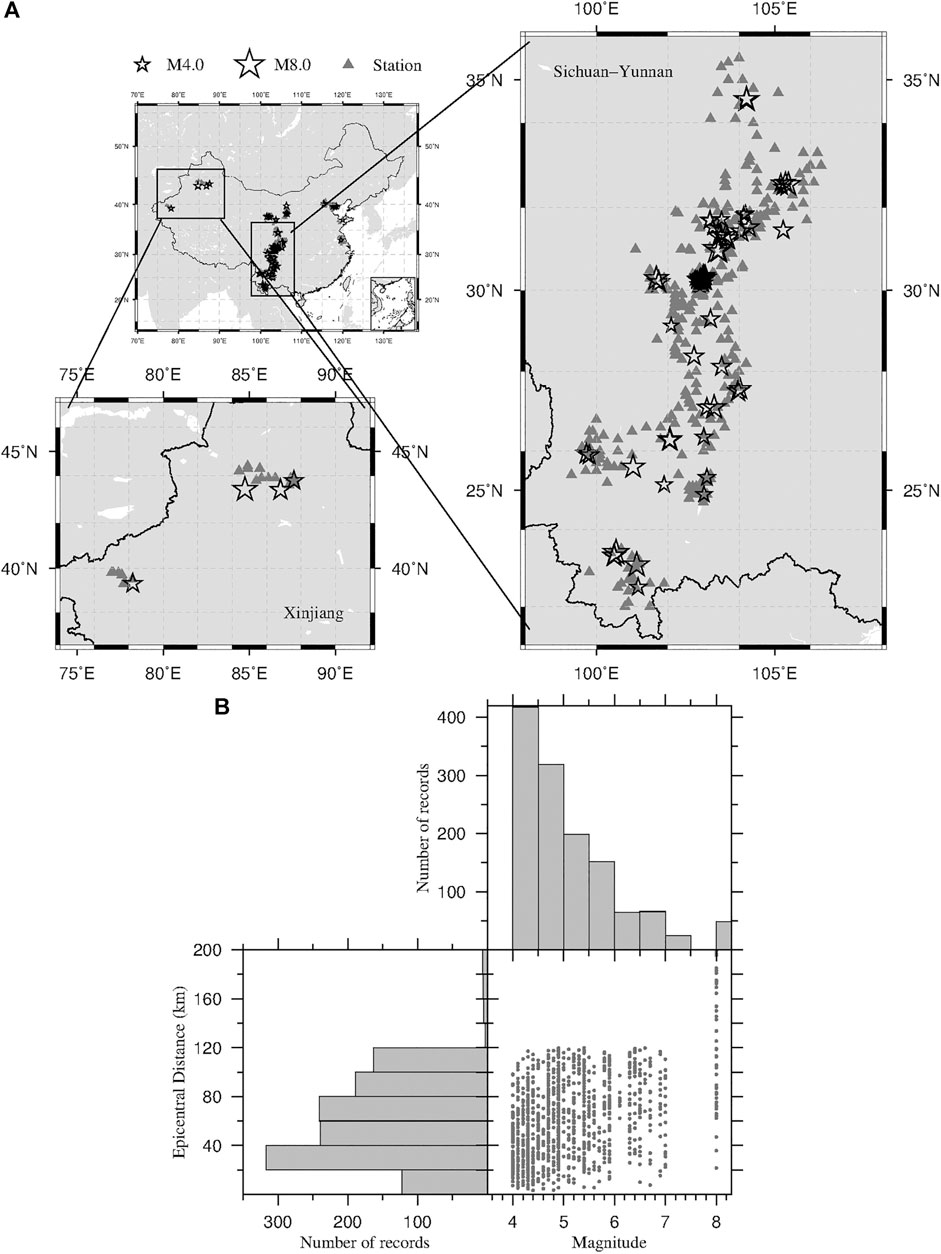
FIGURE 1. Data distribution. Plot of (A) the epicentral position of the selected earthquakes and the location of stations and (B) the distribution of the analysed records as a function of the epicentral distance and magnitude.

We identified the onset of the P wave on the vertical component of acceleration records, using a standard short-term/long-term average method for automatic picking (Allen, 1978). Then, we visually inspected all the available waveforms and made manual picks where necessary, to adjust potential mistakes from the automatic picking algorithm. After removing the mean value and the linear trend, the acceleration waveforms are integrated once to velocity and twice to get displacement. Finally, we applied a 0.075 Hz high-pass Butterworth filter to remove the low frequency drift on displacement records. We impose the zero-crossing of the signal amplitude at the onset of the P-wave, to eliminate any potential residual noise contaminations resulting from the double integration operation.

We then measure the absolute maximum of the initial P-wave amplitude on the vertical component of displacement (named Pd) using an expanding time window, starting at the arrival of the P-wave and moving forward with a time step of 0.01 s. The peak amplitude is related to the earthquake magnitude (M) and to the source-to-receiver distance (R) through an attenuation relationship of the general form (Wu and Zhao, 2006; Zollo et al., 2006):

$\mathit{lo}{\mathit{g}}_{10}\left(\mathit{Pd}\right)=\mathit{A}+\mathit{BM}+\mathit{Clo}{\mathit{g}}_{10}\left(\mathit{R}\right)(1)$

where Pd is the P-wave peak measurements and A, B and C are coefficients empirically determined from select dataset using 2 or 3 s after the P-wave arrival. Unlike the previous study, here we calibrated the coefficients by performing a specific least-squares multiple regression analysis, in which we fixed the distance attenuation coefficient (C) and chose a fixed length of the P-wave time window for the parameter measurements, which was set at 3 s for M $\le$ 7 and 9 s for 5.5 $<$ M $\le$ 7, respectively. Further details about the estimation of the coefficients of Eq. 1 are provided in Supplementary Material.

For the computation of the LPDT curve of each event, the peak amplitudes Pd of all records are measured at every P-wave time window and the distance-corrected amplitudes (logP^cd) are obtained as logP^cd = logPd − ClogR. In order to avoid the contamination by the S-waves on the selected portion of the P-wave, we picked out four stations with clear seismic phase randomly from the dataset in each distance bin (every 20 km). A total number of 40 records were used, and their S-wave arrival time were manually picked to estimate the coefficients of the following equation:

${\mathit{T}}_{\mathit{S}}-{\mathit{T}}_{\mathit{P}}=\mathit{bR}(2)$

where Tp is the P-wave onset time, Ts is the arrival time of the S-wave, R is the hypocentral distance in km, b = 0.13 is the coefficient derived from a linear regression analysis. To minimize any potential S-wave contamination, we regarded Tp+0.8bR as the expected S-wave arrival. As the time window increases, the stations with the expected S-wave arrivals were automatically excluded to make sure only P-wave part involved in the computation. Finally, the LPDT curve is obtained by averaging the distance-corrected amplitude of all the valid stations at each time window. The computation of the curves stops when the number of stations is less than a minimum of data (Five stations).

Observation and Modelling of LPDT Curve

Figure 2 shows an example of the generated LPDT curve for the M4.6 event. The LPDT curve has an exponential growth shape with an initial increase, a gradual intermediate curvature and a final plateau level. Generally, the LPDT curve of larger event needs more time to reach the plateau and the plateau level of the curves scale with the final magnitude (Figure 3A).

FIGURE 2

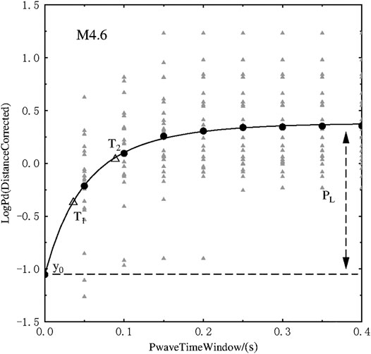
FIGURE 2. The LPDT curve of M4.6 event and the model parameters. The grey triangles stand for the corrected amplitude Pd^C for the available stations at each P-wave time window, then the circle represents the average Pd^C value of all these stations. Our exponential fit model is shown in black line. The time parameters T₁ and T₂ are shown in the empty triangles.

FIGURE 3

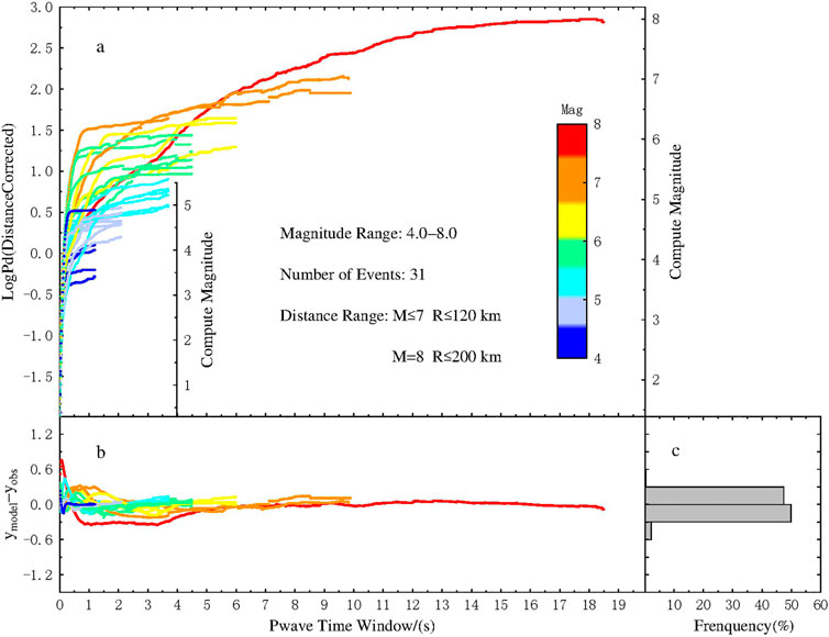
FIGURE 3. The LPDT curve and the misfit. (A) The average peak amplitude with distance corrected at each P-wave time window for different magnitude with color scale. (B) The difference between the observed value and the value from the fit model. (C) The normalized histograms of the misfit value.

The shape of the LPDT curve, as obtained from the average of many stations distributed over azimuth and distance, can be interpreted as a proxy of the Moment Rate Function (MRF), from the initial time up to its maximum peak value. Therefore, two essential features of the MRF, i.e., peak value and peak time, which are both related to the source properties, should be embodied in the LPDT curves. Following the idea of Colombelli and Zollo (2015), for near-triangular source time functions, the peak value of the MRF (related to the magnitude) will correspond to the plateau level of the LPDT curve, and the peak time of the MRF (related to rupture half-duration) is a proxy for the time at which the LPDT curve reaches its plateau level (Plateau Time). With this in mind, the magnitude and rupture duration can be estimated from the plateau level and the plateau time of the curves.

To model the LPDT curves, we fit data using the following function (Colombelli et al., 2020):

$\mathit{lo}{\mathit{g}}_{10}\mathit{Pd}\left(\mathit{t}\right)={\mathit{P}}_{\mathit{L}}\left\{1-\left[\mathit{a}{\mathit{e}}^{-\frac{\mathit{t}}{{\mathit{T}}_1}}+\left(1-\mathit{a}\right)\left({\mathit{e}}^{-\frac{\mathit{t}}{{\mathit{T}}_2}}\right)\right]\right\}+{\mathit{y}}_0(3)$

where y₀is fixed as the first point of the curve,P_L is the interval between y₀and the plateau level, a is the weighting factor which is set to 0.5,T₁, and T₂ are the time parameters (here we define the larger value as T₂). T₁ controls the very initial part which usually has a faster increasing speed and T₂ represents the second part, whose increasing speed gradually becomes slower. This double corner time, exponential model accounts finely for the two different behaviors of LPDT curve-that is to say, a sharp increase to the plateau (ramp-like) for small events and a more gentle and smooth increase (exponential) for large events. The model parameters are shown in Figure 2.

We used a non-linear, weighted-fitting approach to model our curves, accounting for the standard error on each point of LPDT curves. Specifically, at each time step, the weight is obtained as:

$\mathit{Weight}=1/\left(N\cdot S{E}^2\right)(4)$

where SE is the standard error in each P-wave time window, N is the number of stations used for that time window. Figure 3B shows that the LPDT curves of all the events are quite well reproduced by the fitting model, with an average residual of 0.3. Generally, at the beginning of the curve computation, several stations from a broad range of distances and azimuths are involved in the calculation, so that the scatter of data is large and the fitting procedure gives a smaller weight to this part, as compared to the plateau of the curves, which is instead, well reproduced. A slightly larger (about 0.7) difference between the real data and the model is observed for the initial part of the curve of the M 8.0 Wenchuan earthquake, which could be related to the complexity of the source process of this peculiar event. Indeed, when looking at the seismic moment release of this event (Figure 4), a small peak value is observed at 4–5 s, before the arrival of the absolute main peak value (at about 25 s), and this leads to a sag of the LPDT curve around 4 s.

FIGURE 4

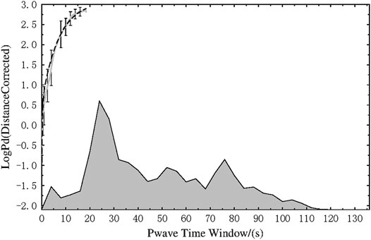
FIGURE 4. The LPDT curve of the M 8.0 Wenchuan earthquake and its fit model. The grey and the dashed line represent the observed data and the best fit model, respectively. The standard error of the corrected amplitude Pd^C for the available stations at each P-wave time window is shown by the vertical error bars. The moment rate function of this event provided by the USGS was shown in the bottom with grey area.

Results

We fit the LPDT curves with our exponential model and obtain the three relevant parameters mentioned above (T₁, T₂, P_L) while y₀ has been fixed to the first point amplitude. For simplicity, we defined a new variable called P_L* = P_L + y₀ to represent the true plateau level of the LPDT curves. Both the amplitude parameter (P_L*) and the two characteristic times (T₁ and T₂) scale with earthquake magnitude. Figure 5 shows the plateau level P_L* as a function of magnitude. A good correlation between P_L* and magnitude (the correlation coefficient reaches 0.95) can be found. The parameters T₁ and T₂ extracted from our fitting model are shown in Figure 6 as a function of magnitude. As the best fitting line indicates, both parameters linearly increase with magnitude (in logarithmic scale). Due to the very rapid initial increase of the curves, T₁ and T₂ are close to each other for small events, while they gradually separate when the magnitude becomes larger and the initial part of the curves increases gently.

FIGURE 5

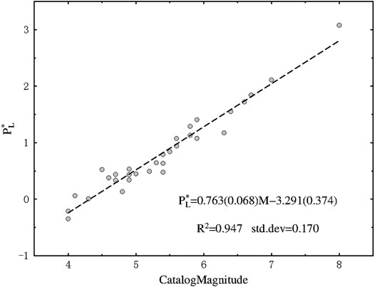
FIGURE 5. Scaling relationship between P_L* and magnitude. The circles present the P_L* value of each event. The dashed line indicates the best-fit relation between P_L* and magnitude.

FIGURE 6

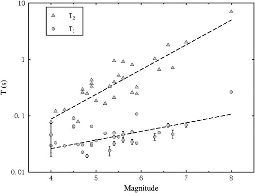
FIGURE 6. Scaling relationship between T₁ and T₂ as a function of magnitude. Triangles and circles represent T₂ and T₁ for LPDT curves, respectively. The error bars which represent the standard deviation of the parameters fitted by our exponential model are shown as black lines (where visible). The best fitting line for each parameter is shown as dashed line.

Magnitude Estimation

Once the observed amplitude has been corrected for the distance effect, the LPDT value at each P-wave time window can be associated to a corresponding magnitude using the coefficients of Eq. 1 (Supplementary Table S1). Figure 3 shows the dynamic process of estimating magnitude for the LPDT curve. The y axis on the left stands for the distance corrected Pd, and the corresponding magnitude or estimated magnitude scale is shown on the right. The magnitude then can be estimated accurately based on the true plateau level of the LPDT curves and the coefficients of Eq. 1 listed in Supplementary Table S1. As shown in Figure 3, the occurrence of the plateau for large events (M > 6–7) needs more than 9 s after the P-wave arrival, suggesting that the typical approaches for the magnitude estimate using fixed 3–4 s P-wave time windows (PTWs) would provide underestimated magnitudes for such large events. Moreover, the B coefficient (calibrated using a 3 s PTW) could not be suitable to compute the corresponding magnitude based on the P_L^* obtained in a longer time window. We therefore choose two magnitude ranges, with two different PTW lengths, to calibrate and use the optimal coefficients (Supplementary Table S1) for magnitude estimation. In this way, when an event reached its plateau within 4 s, we use the relation coefficients A and B for fixed 3 s PTW, while we used the coefficients A and B established with a fixed 9 s PTW when its LPDT curve keeps increasing after 4 s.

The estimated final magnitude based on the P_L* for the LPDT curve and obtained with the two sets of coefficients for small and large events respectively, is plotted in Figure 7 as a function of the catalog magnitude. As it can be seen in Figure 7, most of the points are distributed around the dashed line representing the 1:1 relationship between the estimated magnitude and the catalog magnitude. The scatter of data is rather small, with an average estimated error of 0.23 magnitude units.

FIGURE 7

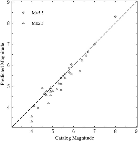
FIGURE 7. The estimation of the magnitude and catalog magnitude. The dashed line corresponds to the 1:1 scaling. The triangles and circles indicate the estimated magnitude with P_L* using the relation coefficients A and B for a fixed 3 s PTW and a fixed 9 s PTW, respectively.

Prediction of Rupture Length and Estimation of Stress Drop Δσ

The rupture duration is the total duration of a seismic event, given by the whole-time length of the moment rate function (Vallée, 2013). It is generally observed that the rupture duration scales with magnitude and is related to the rupture length, assuming a value for the rupture velocity (Wells and Coppersmith, 1994). As the moment rate function can be simplified as a symmetric triangle (Bilek et al., 2004), the peak time of the MRF, corresponding to the plateau time (T_PL) of the LPDT curve, is a measure of the Half-duration of each event (Colombelli and Zollo, 2015; Nazeri et al., 2019). Having in mind the Sato & Hirasawa model (Sato and Hirasawa, 1973) here we investigate the relation between parameter T₂ of LPDT curves and T_PL, the time at which occurs the peak of the MRF. In the Sato & Hirasawa model, the rupture spreads radially outwards at a constant velocity with a circular fault, and stress drop (Δσ) and rupture velocity (Vr) are two relevant parameters controlling the earthquake rupture process. Since Δσ and Vr of earthquakes can vary significantly for each event (Allmann and Shearer, 2009), we performed a set of dedicated simulations to explore stress drop values between 0.05 and 20 MPa with rupture velocities between 0.5 Vs (S-wave velocity) and 0.9 Vs, for a total of 55 combinations of the two parameters.

For each given magnitude, we fixe Δσ and Vr, and generate the corresponding Sato & Hirasawa moment rate Function (SHF) by changing the polar angle of the observation point from 0^o to 90^o and computing the average SHF (an example of M = 5 event shown in the Figure 8A). We then compute the log of the SHF and keep unchanged after the SHF reaches its peak to get a curve (hereinafter LSHF) with a similar shape of our LPDT curve. Since most of the selected earthquakes in our database occurred at an average depth of about 10 km, we set the Vp = 6.2 km/s, Vs = 3.4 km/s based on the velocity model for this region (Wang et al., 2014). Examples of the average SHF with fixed Vr = 0.7 Vs and Δσ = 0.1 MPa is shown in Figure 8, while examples with other Δσ values are shown in the Supplementary Material. For each available couple of stress drop and rupture velocity, we used the exponential model (Eq. 3) to fit the LSHF curve and extract the T₂ parameter for different magnitudes. As expected, we found that T₂ has linear relationship with T_PL obtained directly from the peak time of the generated SHF (in logarithmic scale) for the entire magnitude range with a small deviation when exploring the Δσ and Vr, suggesting that the T₂ parameter extracted from the observed curves can be used to predict T_PL:

$\mathit{lo}{\mathit{g}}_{10}\left({\mathit{T}}_{\mathit{PL}}\right)=1.111\left(0.051\right)\mathit{lo}{\mathit{g}}_{10}\left({\mathit{T}}_2\right)+0.542\left(0.030\right)(5)$

FIGURE 8

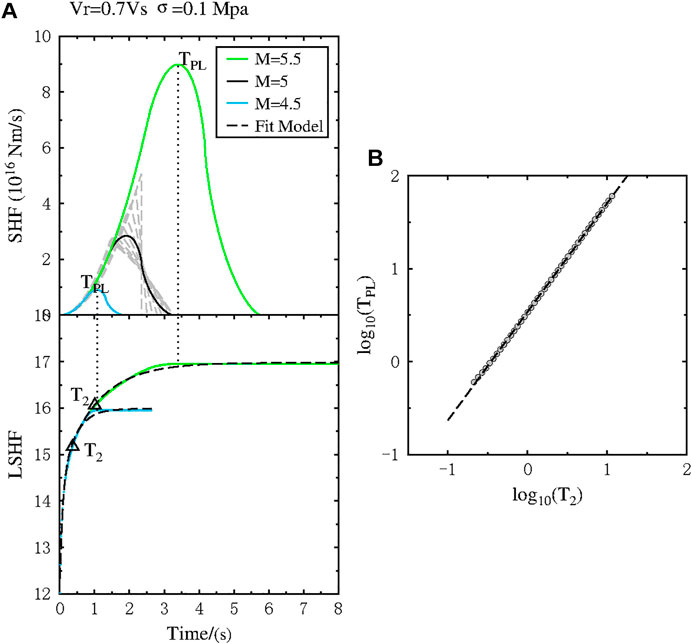
FIGURE 8. The exploratory simulations for Δσ = 0.1 MPa. (A) Fitting of the Sato & Hirasawa function with exponential model. The SHF and LSHF stand for the Sato & Hirasawa moment rate Function (SHF) and the log of the SHF (LSHF), respectively. The grey hatched curves display different SHFs, obtained by changing the polar angle of the observation point from 0^o to 90^o. The black solid line shows the average SHF for M = 5 event. The blue and green line represent the averaged SHF for M = 4.5 and M = 5.5 event, respectively. The dashed line represents the fitted model. (B) Relationship between T₂ and T_PL for magnitude from 4 to 8 with an interval of 0.1 magnitude units. The dashed line shows the fitting relationship between T₂ and T_PL.

For the circular model with a symmetric triangular shaped MRF, the obtained T_PL can be regard as the Half-Duration (HD) of the source function. Considering all azimuthal coverage around the fault, the relation between averaged half-duration and the source radius was given as follows (Aki and Richards, 2002):

${\mathit{T}}_{\mathit{PL}}=\langle \mathit{HD}\rangle =\frac{{\displaystyle {\int }_0^{\frac{\mathit{\pi }}{2}}\frac{\mathit{a}}{{\mathit{V}}_{\mathit{r}}}\left(1-\frac{{\mathit{V}}_{\mathit{r}}\mathit{sin\theta }}{{\mathit{V}}_{\mathit{P}}}\right)\mathit{d\theta }}}{\frac{\mathit{\pi }}{2}}=\frac{\mathit{a}}{{\mathit{V}}_{\mathit{r}}}\left(1-\frac{2}{\mathit{\pi }}\frac{{\mathit{V}}_{\mathit{r}}}{{\mathit{V}}_{\mathit{P}}}\right)(6)$

where a is the source radius, Vr is rupture velocity, $\mathit{\theta }$ is the polar angle of the observation point and Vp is the P-wave velocity. Given the half-duration of the source, the source radius of the analysed events can be estimated.

Figure 9 shows the predicted source radius as a function of magnitude and its corresponding half-duration with a fixed rupture velocity of 0.9 Vs. Based on the computation of stress drop (Δσ) for the circular model using the source radius (a) and the seismic moment (M₀) (Keilis-Borok, 1959), $\mathrm{\Delta }\sigma =\frac{7}{16}\frac{{\mathit{M}}_0}{{\mathit{a}}^3}$, the theoretical scaling lines of the source radius as a function of M with a constant Δσ = 0.1 and 10 MPa were given in the same figure as a comparison. The predicted source radius shows a similar increasing trend with the theoretical lines, indicating that the source radius of the analysed events has a consistent self-similar, constant stress drop scaling with magnitude. We fit the source radius with a weight-based fitting approach (same as Eq. 4, here, the SE is the standard error of the source radius computed from the predicted T_PL and its error obtained by the error propagation theory) to obtain the best-fit constant stress drop of 0.4 MPa. In addition, we repeated the process by setting Vr = 0.7 Vs and Vr = 0.8 Vs, and found that the mean value of Δσ are 1.0 and 0.6 MPa, respectively.

FIGURE 9

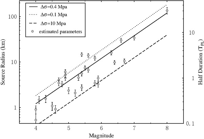
FIGURE 9. The scaling relation between source radius and magnitude with a fixed rupture velocity of 0.9 Vs. The right y-axis represents the corresponding Half-duration. The circles stand for the T_PL parameter extracted from LPDT curve. The estimated errors computed through the error propagation theory are shown by the vertical error bars. The dotted line and dashed line represent the theoretical scaling with constant Δσ = 0.1 and 10 MPa, respectively. The averaged constant Δσ of the analysed dataset are shown in the solid line.

The definition of rupture length changes in case of a circular fault (rupture length = rupture radius) and long-rectangular fault (rupture length = larger rectangular fault dimension). For a circular fault, the rupture lengths (source radius) predicted from LPDT curve were shown in Figure 10. As the figure indicates, most of our predicted rupture lengths as a function of magnitude agrees with the magnitude-rupture scaling relation studied by Cheng et al. (2019) using 91 earthquakes in Mainland China and the empirical scaling relation for strike-slip earthquakes with M 4.8 to M 8.1 proposed by Wells and Coppersmith (1994). However, our predicted results were smaller than the rupture length of two models in the moderate-large magnitude range (M 7.0 Lushan earthquake and M 8.0 Wenchuan earthquake). To better assess the performances of our LPDT scheme in predicting rupture length, we collect the rupture lengths of these two largest events derived from other methodologies. Our approach provides a rupture length of 34 km for the M 7.0 Lushan earthquake, which is consistent with the results of relocated aftershocks by Fang et al. (2013) (L∼35 km) and the inversion results by Liu et al. (2013) (L∼28 km). For the M 8.0 Wenchuan earthquake, our predicted rupture length of 135 km is obviously underestimated as compared to the inversion results of Zhang et al. (2014) (L∼300 km) and the observed aftershock distribution over a length of 330 km (Huang et al., 2008).

FIGURE 10

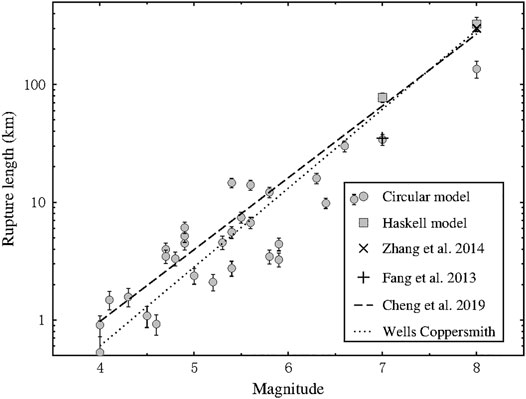
FIGURE 10. The scaling relationship between the predicted rupture length and M. The circles and the squares are the predicted rupture length from circular model and Haskell model, respectively. The dashed line is the linear regression relationship in mainland China calibrated by Cheng et al. (2019). The dotted line represents the relationship proposed by Wells and Coppersmith (1994). The diagonal cross and cross are the results of M 8.0 Wenchuan earthquake by Zhang et al. (2014) and M 7.0 Lushan earthquake by Fang et al. (2013), respectively. The estimated errors computed through the error propagation theory are shown by the vertical error bars.

The circular model is well suitable for small-to-moderate magnitudes (i.e., M < 6). Here, we also investigated the results of large magnitudes when applying the rectangular source model of Haskell. The far-field displacement radiated by a Haskell type fault model is equivalent to the convolution of two box-car functions of different amplitude and durations: rise time (τ) and rupture time (T_R). The resulting function has a trapezoidal shape with total duration given by the sum of τ + T_R. The rupture time T_R depends on the finite length of the fault (L) and the azimuth ($\theta$) between source and receiver (Haskell, 1964):

${\mathit{T}}_{\mathit{R}}=\frac{\mathit{L}}{{\mathit{V}}_{\mathit{r}}}\left(1-\frac{{\mathit{V}}_{\mathit{r}}}{{\mathit{V}}_{\mathit{P}}}\mathit{cos\theta }\right)(7)$

The rise time τ is independent of azimuth (Hwang et al., 2011) and can be obtained using the following relationship derived by Melgar and Hayes (2017) from a database of finite faults:

$\mathit{lo}{\mathit{g}}_{10}\left(\mathit{\tau }\right)=-5.323+0.293\mathit{lo}{\mathit{g}}_{10}\left({\mathit{M}}_0\right)(8)$

Figure 11 shows an example of the average total duration of Haskell model with azimuth ($\theta$) changed from 0^o to 180^o. Assuming that T_PL is the middle point of the average trapezoid plateau, the following relationship between L and T_PL can be obtained and be used for estimating rupture length of large events when assuming the Haskell model:

${\mathit{T}}_{\mathit{PL}}=\frac{1}{2}\left(\mathit{\tau }+\frac{\mathit{L}}{{\mathit{V}}_{\mathit{r}}}\left(1-\frac{{\mathit{V}}_{\mathit{r}}}{{\mathit{V}}_{\mathit{P}}}\right)\right)(9)$

FIGURE 11

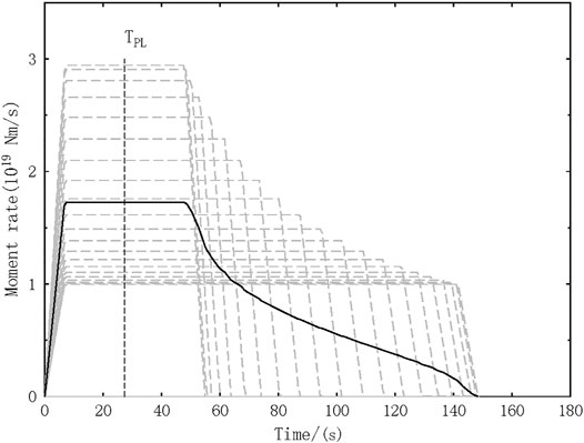
FIGURE 11. The trapezoid-like moment rate function (MRF) and the averaged MRF with azimuth from 0^o to 180^o. The dashed black line represents that the T_PL of the LPDT curves (Plateau time) occurs at the middle point of the average trapezoid plateau.

We computed the predicted rupture length for the two largest events using the Haskell model. As shown in Figure 10, with the same T_PL, applying the Haskell model appears to predict larger rupture lengths than the results using circular model. Specifically, we obtain an estimate of rupture length of 326 km without underestimation for Wenchuan earthquake, whereas the rupture length of Lushan earthquake has been overestimated (L = 77.3 km). The circular model produced a triangle-like MRF, as the Sato & Hirasawa moment rate Function of M = 5 event shown in the Figure 8A indicates, the peak time (T_PL) is almost half-duration. However, as the MRF of M 8.0 Wenchuan earthquake (download from USGS, shown in Figure 4) indicates, the MRF of some large events usually have the major peak occurring at the beginning of the rupture and followed by a long-time duration coda (Vallée, 2013). In this case, the circular model with a triangle-shape MRF may be not able to correctly reproduce this kind of source time function, and considering the peak time as the half-duration of the large events may result into underestimated rupture lengths. The averaged MRF from Haskell model shown in Figure 11 reaches its peak (T_PL) around 1/5 of the total duration, which is more like the characteristic of MRF of the large magnitude earthquakes stated above. Moreover, for large earthquakes, the width (W) of the fault is already saturated, i.e., equal to the thickness of the brittle fracturing zone in the lithosphere. Accordingly, the growth of the fault area with increasing seismic moment (M₀) is in the length direction only (Bormann et al., 2009; Cheng et al., 2019). Therefore, in the situation of L >> W for large events, the Haskell model is more appropriate. Since the rupture surface of Lushan earthquake presents the focal characteristics of small-moderate earthquakes (L ≈ W) (Chen et al., 2013; Hao et al., 2013), the Haskell model is not suitable for this event leading to an overestimated rupture length.

According to the derived rupture length of the analysed events, the stress drop can be computed based on different geometrical faults. Madariaga (1977) proposed that the general form $\Delta \sigma =\frac{M_o}{CSW}\cong \frac{M_o}{C{S}^{3/2}}$ (S is the rupture surface), where $C=\frac{16}{7\pi }$ for a circular fault, same as Keilis-Borok (1959)’s formula $\Delta \sigma =\frac{7}{16}\frac{M_0}{a^3}$ and $C=\frac{\pi }{2}$ for a long rectangular fault (L >> W) as follows:

$\Delta \mathit{\sigma }=\frac{2}{\mathit{\pi }}\frac{{\mathit{M}}_0}{{\mathit{W}}^2\mathit{L}}(10)$

where W is the rupture width. Referring to the observation of Cheng et al. (2019) that large events with M > 6.7 have a nearly constant rupture width of ∼20 km, here, we set W to 20 km.

We therefore suggest to use the circular model for small-moderate-strong events (M $\le$ 7) and the Haskell model (rectangle model) for large events (M > 7) in the estimation of rupture length and stress drop. The computed stress drop of each event is shown in Figure 12. After applying the rectangle source model for M 8.0 Wenchuan earthquake, the derived stress drop = 4.9 MPa is comparable with the results of Meng et al. (2019) (3.5 MPa). However, the circular model in this study provides an underestimated stress drop of 0.4 MPa for M 7.0 Lushan earthquake when comparing with the results (1.8 MPa) obtained by Li et al. (2017). As Figure 12B shows, the stress drops vary from 0.01 to 10 MPa. We divide the events into two groups based on Δσ = 0.6 MPa and calculate the averaged stress drop for these two groups. The higher stress drop group (Δσ > 0.6 MPa) has an averaged stress drop of 3.7 MPa, which is close to the world-wide measured median value of 4 MPa (Allmann and Shearer, 2009). The lower stress drop group with an averaged stress drop of 0.2 MPa consists of 19 events, in which half of the events are the aftershocks of the M 8.0 Wenchuan earthquake and the M 7.0 Lushan earthquake. Consistent with Wang et al. (2018), the lower stress drop of aftershocks may result from the remaining locked parts on the fault plane of the mainshock. All these source parameters of the analyzed events (M $\ge$ 5.5) are summarized in Table 1.

FIGURE 12

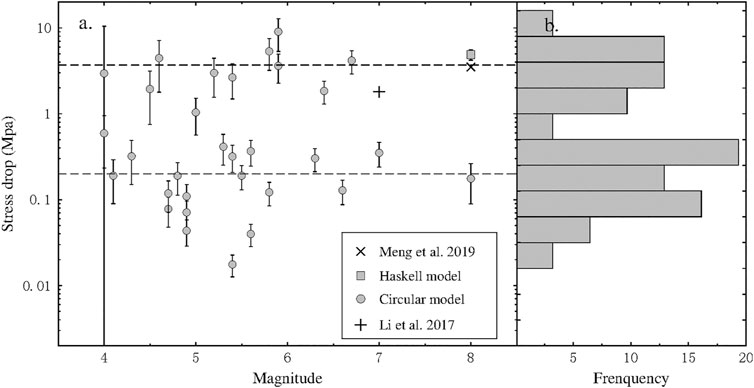
FIGURE 12. The estimated stress drop of the analyzed earthquakes. (A) The distribution of the estimated stress drop. The circles and the squares are the predicted stress drop from circular model and Haskell model, respectively. The estimated errors computed through the error propagation theory are shown by the vertical error bars. Events have been divided into two groups based on Δσ = 0.6 MPa. The average stress drops of these two groups are shown as the dashed lines. The diagonal cross and cross are the results of M 8.0 Wenchuan earthquake by Meng et al. (2019) and M 7.0 Lushan earthquake by Li et al. (2017), respectively. (B) The normalized histograms of the predicted stress drop.

TABLE 1

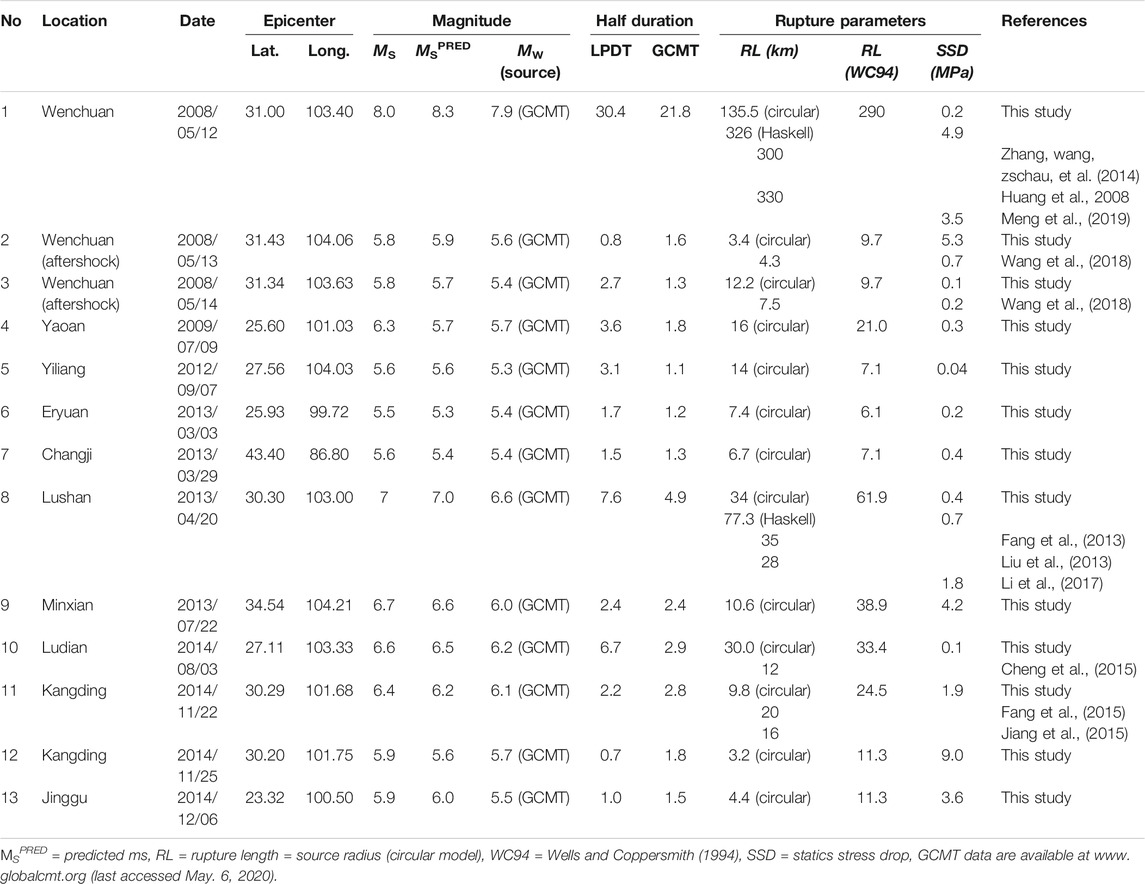
TABLE 1. List of source parameters including catalog magnitude (Ms), predicted magnitude (Ms^PRED), half duration, Rupture length (RL) and stress drop (Δσ) determined in this study for moderate-larger events (M$\ge$ 5.5).

Discussion and Conclusion

In this study, we generalized the approach proposed by Colombelli and Zollo (2015) to estimate the source parameters of a set of Chinese earthquakes with magnitude ranging from 4 to 8. The methodology is based on the use of the time evolution of the P wave (LPDT curve) as a proxy for the source time function to extract earthquake magnitude and rupture duration.

Comparing with the previous works by Colombelli and Zollo (2015) and Nazeri et al. (2019), we used the double corner time, exponential model proposed by Colombelli et al. (2020) for better modeling the behavior of LPDT curves. We improved the magnitude estimation based on the plateau level of LPDT curve, by using two different scaling coefficients with fixed C, which have been properly calibrated. Based on the analysis of 31 events in the magnitude range between 4 and 8, we found that the plateau level of LPDT curves has a strong correlation with magnitude (the coefficient of correlation is up to 0.95). Comparing with the catalog magnitude of the analyzed events, our predicted magnitude from the displacement data shows an average deviation of 0.23 magnitude units. The time at which these estimates are available implicitly depends on the event itself. Small events have a rapid initial increase and reach the plateau quickly, and for these events, the magnitude estimates would be available within a short time from the first P-wave detection. For the large events, like Wenchuan earthquake (M 8.0), the time needed to reach the plateau is longer. The near-source stations with a short fraction portion of the P-wave time-series cannot provide robust magnitude estimates for these large events, which is consistent with our observation that the LPDT curve at this stage is still growing and the plateau has not yet been reached. However, the expansion of hypocentral distance allows to capture longer P-wave signal portion of large events, and thus we provide a magnitude estimation of 8.3 for the Wenchuan earthquake after the LPDT curve reaches its plateau. By capturing the curve that reaches its plateau or looking at larger distances, our approach can estimate the magnitude of large events accurately, without saturation effects, typically observed when using shorter P-wave time windows (Lomax and Michelini, 2009; Bormann and Saul, 2009; Colombelli et al., 2012).

Together with the plateau level, the plateau time (T_PL) of the LPDT curve has also a clear scaling with magnitude, being approximately related to the half-duration of the source. In order to estimate the plateau time, we performed a series of simulations based on the Sato and Hirasawa (1973) circular rupture model and on the assumption that T_PL corresponds to the peak time of the MRF. We generated a set of MRFs exploring Δσ and Vr values and studied the relation between T_PL and the time characteristic parameter T₂. Finally, we established a linear scaling relationship between the two parameters for predicting the T_PL.

Considering the circular model with a symmetric triangular-shaped MRF, the obtained T_PL can be regarded as the Half-Duration (HD) of the events to predict the source radius. The obtained source radius in this study shows a consistent self-similar, constant stress drop scaling with magnitude. We obtained the best-fit stress drop (0.4 MPa) for the 31 analysed events, with fixing rupture velocity to 0.9 Vs. This value is lower than world-wide measured median value of 4 MPa (Allmann and Shearer, 2009), but it is comparable with the mean value of 0.5 MPa by studying the strong-motion recordings of the Wenchuan aftershocks (2008–2013) (Wang et al., 2018).

One major result of this paper concerns the determination of the scaling law of earthquakes in China. We obtained the rupture length of the analysed events using circular model and found the M 8.0 Wenchuan earthquake has a shorter predicted rupture length with comparing to other results. We realize that for the largest events in the sequence, the circular fault model may underestimate the total rupture length. Thus, we suggested to estimate the rupture length of the large events (M > 7) assuming the Haskell, rectangular fault model. Our predicted rupture length of different source models as a function of M is close to the rupture scaling relationship proposed by Cheng et al. (2019) and Wells and Coppersmith (1994).

The most critical issue of the proposed methodology is to assume a triangular shape to represent the source function. The assumption of a circular fault model can be inadequate to describe the complexity of the source for large events, for which multiple peaks of moment release can occur. Moreover, the rupture process of an earthquake is a chaotic process, and the simple exponential LPDT curve may hardly represent the complex nature of this process, especially at the very beginning. However, the now massive and well documented observation of LPDT empirical curves analysed in many worldwide seismic regions and in a wide magnitude and distance range confirm that the general ramp-like behavior of the curves is a universal evidence (Colombelli et al., 2012; Colombelli et al., 2015; Colombelli et al., 2020; Melgar et al., 2015; Trugman et al., 2019) which is well matched by the chosen exponential model (Colombelli et al., 2020). When the curve has reached its peak, the schematic representation with two parameters (plateau time and amplitude), may properly catch the essential features of the process we are interested in.

Concerning the anelastic attenuation effect on LPDT curves, the overall features of the curves are essentially dominated by the event magnitude, which mainly controls the plateau level and the time to reach this plateau, for each curve. Using similar LPDT curves, Colombelli et al., (2020) recently investigated the effect of anelastic attenuation on the shape of the curves. This was done both theoretically and through a careful and detailed analysis of real earthquake data. They found that the chosen anelastic attenuation parametrization (Eq. 1) is appropriate to correct the distance attenuation effect on LPDT curves and this does not produce a systematic effect on plateau and T_PL parameter determination in all the observed curves in the same distance range.

The source parameters of the larger events are a major focus of - and motivation for - the proposed methodology. Although the selected dataset has a relatively wide magnitude range from 4.0 to 8.0, there is an obvious lack of large-magnitude data for events with magnitudes between 7 and 8. The proposed methodology would be better verified through the application to other seismic areas, once that the proper calibration of scaling coefficients has been done. It is worth to mention that the findings (e.g., rupture scaling relation and stress drop distribution) obtained through applying the methodology to the selected events (31 earthquakes) are mainly based on the data from Sichuan-Yunnan region, and may not be applicable to other areas as they are.

We notice that in the presence of a jump in the increasing shape of the LPDT curve, our approach likely fits the curve with a longer T₂ thus resulting in a lower stress drop value. Supplementary Figure S2 shows the LPDT curve for the M 6.6 Ludian earthquake: a jump in the curve is clearly visible around 3.5 s. A similar magnitude event (M 6.4) which has a normal LPDT curve shape without jumps is selected for comparison. Our double corner time, exponential model (Eq. 3) fits the LPDT curve of this M 6.4 event with a T₂ = 0.66 s. However, due to the presence of jump, our exponential model tends to find a parameter (T₁ and T₂) with slower growth to fit the middle part (2 ∼ 4 s) of the LPDT curve for M 6.6 Ludian earthquake. This resulted in our model fitting the LPDT curve with a longer T₂ = 1.8 s. We further justify the effect of LPDT curve shape on the exponential fitting model in Supplementary Figure S3. The virtual LPDT curve with normal LPDT curve shape was generated as follow: the initial increasing part (0 ∼ 1.85 s) and the approach plateau part (4.26 ∼ 6 s) are the same as the observed LPDT curve, and only the middle part, we add points with exponential growth. After using our exponential model to fit the curves separately, we obtained a T₂ = 1.46 s for the virtual LPDT curve with a normal shape and a slightly longer T₂ (1.8 s) for the observed LPDT curve with a jump in the middle. Thus, based on the relationship between T₂ and T_PL, the predicted T_PL (plateau time) of LPDT curve with normal shape then will be 5.3 s, whereas the T_PL of the LPDT curve with jump will be 6.7 s. The jumps on the curve can be given by different effects, both related to the source process itself, such as multiple peaks on the Moment Rate Function, and/or to propagation effects, such as the arrival of intermediate phases (preceding the S-wave arrival), arriving at a receiver within the coda of P-wave phase. However, the presence of jumps on the LPDT curves is not frequently observed in our catalogue, only happens in two events. Meanwhile, the jump in the LPDT curve does not have a serious impact on the derived parameters. Thus, we believe that, on average, this is a negligible effect on the overall estimation of rupture length and stress drop.

The shape of the curves may change in real-time, when we do not have all the available stations. As a perspective of the work, we could evaluate the feasibility of application in real-time, that can be relevant for EEW applications. The accurate estimation of the rupture extent and magnitude at the early stage of the process can be a useful piece of information to add to the early shake-map computation, and the estimation of ground shaking can be strongly improved by considering the effect of the finite fault (Colombelli et al., 2013). While in this off-line study we used the post-earthquake location instead of the real-time estimation, a reliable estimation of the earthquake location is needed for the real-time application. Having in mind that the far-field stations must wait enough time to reach the plateau of the curve for large events, we need more time to get the plateau information. Hence, the real-time application performance and the timeliness based on the network distribution for this approach will be further studied. A possible method could be that we can estimate the final curve at each time step with a given probability and study the real-time curve reached how many percent of the final curve (maybe after T₂) can give a reliable probability for estimating final curve.

Data Availability Statement

The original contributions presented in the study are included in the article/Supplementary Material, further inquiries can be directed to the corresponding authors.

Author Contributions

YW applied the methodology and drafted the manuscript; SC and AZ critically revised the paper and supervised the study; JS and SL provided suggestions on the results. All authors contributed to the article and approved the submitted version.

Funding

This research was financially supported by the National Key Research and Development Program of China (2018YFC1504003) and its provincial funding, the Italian Ministry of Research and the University of Naples Federico II (Project Number AIM1834927-3; E66C19000090001), and the Scientific Research Fund of Institute of Engineering Mechanics, China Earthquake Administration (2016A03).

Conflict of Interest

The authors declare that the research was conducted in the absence of any commercial or financial relationships that could be construed as a potential conflict of interest.

Acknowledgments

We thank the China Strong Motion Network Centre (CSMNC) at the Institute of Engineering Mechanics, China Earthquake Administration, for providing the ground motion recording data. We would like to thank the University of Naples Federico II where the work has been carried out during the visiting period. We would also like to thank Jia Cheng (Institute of Crustal Dynamics, China Earthquake Administration) for the discussion about the calculation of stress drop. The moment rate function of the M 8.0 Wenchuan earthquake has been provided by the USGS: https://earthquake.usgs.gov/earthquakes/eventpage/usp000g650/finite-fault (last accessed May 2020). This manuscript has been posted on Earth and Space Science Open Archive (ESSOAr) with a preprint service (https://www.essoar.org/doi/abs/10.1002/essoar.10503831.1).

Supplementary Material

The Supplementary Material for this article can be found online at: https://www.frontiersin.org/articles/10.3389/feart.2021.616229/full#supplementary-material.

References

Aki, K., and Richards, P. G. (2002). Quantitative seismology. Sausalito, CA: University Science Books.

Allen, R. M., and Kanamori, H. (2003). The potential for earthquake early warning in southern California. Science 300 (5620), 786–789. doi:10.1126/science.1080912

PubMed Abstract | CrossRef Full Text | Google Scholar

Allen, R. M., and Ziv, A. (2011). Application of real-time GPS to earthquake early warning. Geophys. Res. Lett. 38 (16) doi:10.1029/2011gl047947

CrossRef Full Text | Google Scholar

Allen, R. V. (1978). Automatic earthquake recognition and timing from single traces. Bull. Seismological Soc. America 68 (5), 1521–1532.

Google Scholar

Allmann, B. P., and Shearer, P. M. (2009). Global variations of stress drop for moderate to large earthquakes. J. Geophys. Res. 114 (B1). doi:10.1029/2008jb005821

CrossRef Full Text | Google Scholar

Bilek, S. L., Lay, T., and Ruff, L. J. (2004). Radiated seismic energy and earthquake source duration variations from teleseismic source time functions for shallow subduction zone thrust earthquakes. J. Geophys. Res. 109 (B9), a. doi:10.1029/2004jb003039

CrossRef Full Text | Google Scholar

Brune, J. N. (1970). Tectonic stress and the spectra of seismic shear waves from earthquakes. J. Geophys. Res. 75 (26), 4997–5009. doi:10.1029/JB075i026p04997

Google Scholar

Boatwright, J. (1980). A spectral theory for circular seismic sources; simple estimates of source dimension, dynamic stress drop, and radiated seismic energy. Bull. Seismological Soc. America 70 (1), 1–27.

Google Scholar

Bormann, P., Baumbach, M., Bock, G., Grosser, H., Choy, G. L., and Boatwright, J. (2009). “Seismic sources and source parameters,” in New manual of seismological observatory practice (NMSOP). Editor P. Bormann (Potsdam: Deutsches GeoForschungsZentrum GFZ), 1–94.

Google Scholar

Bormann, P., and Saul, J. (2009). “Earthquake magnitude,” in Encyclopedia of complexity and systems science. Editor R. Meyers (New York, N Y: Springer). doi:10.1007/978-0-387-30440-3_151

CrossRef Full Text | Google Scholar

Keilis-Borok, V. (1959). On estimation of the displacement in an earthquake source and of source dimensions. Ann. Geofis. (Rome) 12, 205–214. doi:10.4401/ag-5718

CrossRef Full Text | Google Scholar

Böse, M., Felizardo, C., and Heaton, T. H. (2015). Finite-fault rupture detector (FinDer): going real-time in CalifornianShakeAlertWarning system. Seismological Res. Lett. 86 (6), 1692–1704. doi:10.1785/0220150154

CrossRef Full Text | Google Scholar

Böse, M., Heaton, T. H., and Hauksson, E. (2012). Real-time finite fault rupture detector (FinDer) for large earthquakes. Geophys. J. Int. 191 (2), 803–812. doi:10.1111/j.1365-246X.2012.05657.x

CrossRef Full Text | Google Scholar

Böse, M., Ionescu, C., and Wenzel, F. (2007). Earthquake early warning for Bucharest, Romania: novel and revised scaling relations. Geophys. Res. Lett. 34 (7). doi:10.1029/2007gl029396

CrossRef Full Text | Google Scholar

Caprio, M., Lancieri, M., Cua, G. B., Zollo, A., and Wiemer, S. (2011). An evolutionary approach to real-time moment magnitude estimation via inversion of displacement spectra. Geophys. Res. Lett. 38 (2), a. doi:10.1029/2010gl045403

CrossRef Full Text | Google Scholar

Chen, Y., Yang, Z., Zhang, Y., and Liu, C. (2013). From 2008 Wenchuan earthquake to 2013 Lushan earthquake (in Chinese). Sci. China Ser. D: Earth Sci. 43, 1064–1072.

Google Scholar

Cheng, J., Rong, Y., Magistrale, H., Chen, G., and Xu, X. (2019). Earthquake rupture scaling relations for mainland China. Seismological Res. Lett. 91 (1), 248–261. doi:10.1785/0220190129

CrossRef Full Text | Google Scholar

Cheng, J., Wu, Z., Liu, J., Jiang, C., Xu, X., Fang, L., et al. (2015). Preliminary report on the 3 august 2014, mw 6.2/ms 6.5 ludian, yunnan-sichuan border, southwest China, earthquake. Seismological Res. Lett. 86 (3), 750–763. doi:10.1785/0220140208

CrossRef Full Text | Google Scholar

Colombelli, S., Allen, R. M., and Zollo, A. (2013). Application of real-time GPS to earthquake early warning in subduction and strike-slip environments. J. Geophys. Res. Solid Earth 118 (7), 3448–3461. doi:10.1002/jgrb.50242

CrossRef Full Text | Google Scholar

Colombelli, S., Festa, G., and Zollo, A. (2020). Early rupture signals predict the final earthquake size. Geophys. J. Int. 223 (1), 692–706. doi:10.1093/gji/ggaa343

CrossRef Full Text | Google Scholar

Colombelli, S., and Zollo, A. (2015). Fast determination of earthquake magnitude and fault extent from real-timeP-wave recordings. Geophys. J. Int. 202 (2), 1158–1163. doi:10.1093/gji/ggv217

CrossRef Full Text | Google Scholar

Colombelli, S., Zollo, A., Festa, G., and Kanamori, H. (2012). Early magnitude and potential damage zone estimates for the great Mw 9 Tohoku-Oki earthquake. Geophys. Res. Lett. 39 (22), a. doi:10.1029/2012gl053923

CrossRef Full Text | Google Scholar

Duputel, Z., Rivera, L., Kanamori, H., and Hayes, G. (2012). W phase source inversion for moderate to large earthquakes (1990-2010). Geophys. J. Int. 189 (2), 1125–1147. doi:10.1111/j.1365-246X.2012.05419.x

CrossRef Full Text | Google Scholar

Fang, L., Wu, J., Liu, J., Cheng, J., Jiang, C., Han, L., et al. (2015). Preliminary report on the 22 november 2014Mw 6.1/ms 6.3 kangding earthquake, western sichuan, China. Seismological Res. Lett. 86 (6), 1603–1613. doi:10.1785/0220150006

CrossRef Full Text | Google Scholar

Fang, L., Wu, J., Wang, W., Lü, Z., Wang, C., Yang, T., et al. (2013). Relocation of the mainshock and aftershock sequences of M S7.0 Sichuan Lushan earthquake. Chin. Sci. Bull. 58 (28-29), 3451–3459. doi:10.1007/s11434-013-6000-2

CrossRef Full Text | Google Scholar

Hao, J., Ji, C., Wang, W., and Yao, Z. (2013). Rupture history of the 2013Mw6.6 Lushan earthquake constrained with local strong motion and teleseismic body and surface waves. Geophys. Res. Lett. 40 (20), 5371–5376. doi:10.1002/2013gl056876

CrossRef Full Text | Google Scholar

Haskell, N. A. (1964). Total energy and energy spectral density of elastic wave radiation from propagating faults. Bull. Seismological Soc. America 54 (6A), 1811–1841.

Google Scholar

Heaton, T. H. (1990). Evidence for and implications of self-healing pulses of slip in earthquake rupture. Phys. Earth Planet. Interiors 64 (1), 1–20. doi:10.1016/0031-9201(90)90002-f

CrossRef Full Text | Google Scholar

Hoshiba, M., and Aoki, S. (2015). Numerical shake prediction for earthquake early warning: data assimilation, real‐time shake mapping, and simulation of wave propagation. Bull. Seismological Soc. America 105 (3), 1324–1338. doi:10.1785/0120140280

CrossRef Full Text | Google Scholar

Huang, Y., Wu, J., Zhang, T., and Zhang, D. (2008). Relocation of the M8.0 Wenchuan earthquake and its aftershock sequence. Sci. China Ser. D-earth Sci. 51 (12), 1703–1711. doi:10.1007/s11430-008-0135-z

CrossRef Full Text | Google Scholar

Hwang, R.-D., Chang, J.-P., Wang, C.-Y., Wu, J.-J., Kuo, C.-H., Tsai, Y.-W., et al. (2011). Rise time and source duration of the 2008 M W 7.9 Wenchuan (China) earthquake as revealed by Rayleigh waves. Earth Planet. Sp 63 (5), 427–434. doi:10.5047/eps.2011.01.002

CrossRef Full Text | Google Scholar

Jiang, G., Wen, Y., Liu, Y., Xu, X., Fang, L., Chen, G., et al. (2015). Joint analysis of the 2014 Kangding, southwest China, earthquake sequence with seismicity relocation and InSAR inversion. Geophys. Res. Lett. 42 (9), 3273–3281. doi:10.1002/2015gl063750

CrossRef Full Text | Google Scholar

Kanamori, H. (2005). Real-time seismology and earthquake damage mitigation. Annu. Rev. Earth Planet. Sci. 33 (1), 195–214. doi:10.1146/annurev.earth.33.092203.122626

CrossRef Full Text | Google Scholar

Li, J., Liu, C., Zheng, Y., and Xiong, X. (2017). Rupture process of the M s 7.0 Lushan earthquake determined by joint inversion of local static GPS records, strong motion data, and teleseismograms. J. Earth Sci. 28 (2), 404–410. doi:10.1007/s12583-017-0757-1

CrossRef Full Text | Google Scholar

Li, X., Zhou, Z., Yu, H., Wen, R., Lu, D., Huang, M., et al. (2008). Strong motion observations and recordings from the great Wenchuan Earthquake. Earthq. Eng. Eng. Vib. 7 (3), 235–246. doi:10.1007/s11803-008-0892-x

CrossRef Full Text | Google Scholar

Liu, C., Zheng, Y., Ge, C., Xiong, X., and Hsu, H. (2013). Rupture process of the M s7.0 Lushan earthquake, 2013. Sci. China Earth Sci. 56 (7), 1187–1192. doi:10.1007/s11430-013-4639-9

CrossRef Full Text | Google Scholar

Lomax, A., and Michelini, A. (2009). Mwpd: a duration-amplitude procedure for rapid determination of earthquake magnitude and tsunamigenic potential fromPwaveforms. Geophys. J. Int. 176 (1), 200–214. doi:10.1111/j.1365-246X.2008.03974.x

CrossRef Full Text | Google Scholar

Madariaga, R. (1976). Dynamics of an expanding circular fault. Bull. Seismological Soc. America 66 (3), 639–666.

Google Scholar

Madariaga, R. (1977). Implications of stress-drop models of earthquakes for the inversion of stress drop from seismic observations. Pageoph 115, 301–316. doi:10.1007/bf01637111

CrossRef Full Text | Google Scholar

Melgar, D., Crowell, B. W., Geng, J., Allen, R. M., Bock, Y., Riquelme, S., et al. (2015). Earthquake magnitude calculation without saturation from the scaling of peak ground displacement. Geophys. Res. Lett. 42 (13), 5197–5205. doi:10.1002/2015gl064278

CrossRef Full Text | Google Scholar

Melgar, D., and Hayes, G. P. (2017). Systematic observations of the slip pulse properties of large earthquake ruptures. Geophys. Res. Lett. 44 (19), 9691–9698. doi:10.1002/2017gl074916

CrossRef Full Text | Google Scholar

Meng, L., Zang, Y., McGarr, A., and Zhou, L. (2019). High-frequency ground motion and source characteristics of the 2008 wenchuan and 2013 lushan, China, earthquakes. Pure Appl. Geophys. 177 (1), 81–93. doi:10.1007/s00024-019-02291-4

CrossRef Full Text | Google Scholar

Nazeri, S., Colombelli, S., and Zollo, A. (2019). Fast and accurate determination of earthquake moment, rupture length and stress release for the 2016-2017 Central Italy seismic sequence. Geophys. J. Int. 217 (2), 1425–1432. doi:10.1093/gji/ggz097

CrossRef Full Text | Google Scholar

Ohta, Y., Miura, S., Ohzono, M., Kita, S., Iinuma, T., Demachi, T., et al. (2011). Large intraslab earthquake (2011 April 7, M 7.1) after the 2011 off the Pacific coast of Tohoku Earthquake (M 9.0): coseismic fault model based on the dense GPS network data. Earth Planet. Sp 63 (12), 1207–1211. doi:10.5047/eps.2011.07.016

CrossRef Full Text | Google Scholar

Sato, T., and Hirasawa, T. (1973). Body wave spectra from propagating shear cracks. J,Phys,Earth 21 (4), 415–431. doi:10.4294/jpe1952.21.415

CrossRef Full Text | Google Scholar

Trugman, D. T., Page, M. T., Minson, S. E., and Cochran, E. S. (2019). Peak ground displacement saturates Exactly when expected: implications for earthquake early warning. J. Geophys. Res. Solid Earth 124 (5), 4642–4653. doi:10.1029/2018jb017093

CrossRef Full Text | Google Scholar

Vallée, M. (2013). Source time function properties indicate a strain drop independent of earthquake depth and magnitude. Nat. Commun. 4 (1), 2606. doi:10.1038/ncomms3606

PubMed Abstract | CrossRef Full Text | Google Scholar

Wang, H., Ren, Y., and Wen, R. (2018). Source parameters, path attenuation and site effects from strong-motion recordings of the Wenchuan aftershocks (2008-2013) using a non-parametric generalized inversion technique. Geophys. J. Int. 212 (2), 872–890. doi:10.1093/gji/ggx447

CrossRef Full Text | Google Scholar

Wang, W., Wu, J., Fang, L., Lai, G., Yang, T., and Cai, Y. (2014). Swave velocity structure in southwest China from surface wave tomography and receiver functions. J. Geophys. Res. Solid Earth 119 (2), 1061–1078. doi:10.1002/2013jb010317

CrossRef Full Text | Google Scholar

Wells, D. L., and Coppersmith, K. J. (1994). New empirical relationships among magnitude, rupture length, rupture width, rupture area, and surface displacement. Bull. Seismological Soc. America 84 (4), 974–1002.

Google Scholar

Wu, Y.-M., and Kanamori, H. (2008). Exploring the feasibility of on-site earthquake early warning using close-in records of the 2007 Noto Hanto earthquake. Earth Planet. Sp 60 (2), 155–160. doi:10.1186/BF03352778

CrossRef Full Text | Google Scholar

Wu, Y.-M., and Zhao, L. (2006). Magnitude estimation using the first three seconds P-wave amplitude in earthquake early warning. Geophys. Res. Lett. 33 (16). doi:10.1029/2006gl026871

CrossRef Full Text | Google Scholar

Zhang, Y., Wang, R., Zschau, J., Chen, Y.-t., Parolai, S., and Dahm, T. (2014). Automatic imaging of earthquake rupture processes by iterative deconvolution and stacking of high-rate GPS and strong motion seismograms. J. Geophys. Res. Solid Earth 119 (7), 5633–5650. doi:10.1002/2013jb010469

CrossRef Full Text | Google Scholar

Ziv, A., and Lior, I. (2016). Real‐time moment magnitude and stress drop with implications for real‐time shaking prediction. Bull. Seismological Soc. America 106 (6), 2459–2468. doi:10.1785/0120160091

CrossRef Full Text | Google Scholar

Zollo, A., Amoroso, O., Lancieri, M., Wu, Y.-M., and Kanamori, H. (2010). A threshold-based earthquake early warning using dense accelerometer networks. Geophys. J. Int. 183 (2), 963–974. doi:10.1111/j.1365-246X.2010.04765.x

CrossRef Full Text | Google Scholar

Zollo, A., Lancieri, M., and Nielsen, S. (2006). Earthquake magnitude estimation from peak amplitudes of very early seismic signals on strong motion records. Geophys. Res. Lett. 33 (23). doi:10.1029/2006gl027795

CrossRef Full Text | Google Scholar