Strong-Motions From Damaging Moderate Magnitude (5.9 ≥ Mw) Earthquakes in Japan Recorded by K-NET and KiK-net

Introduction

Big earthquakes are generally well reported and investigated in detail for disaster prevention measures for future earthquakes. It is well known that strong-earthquakes of magnitudes over about six can cause damage to broad areas crossing town and city borders, sometimes resulting in many fatalities: for example, the 2009 Mw 6.3 L’Aquila earthquake that caused fatalities of over 300 people and left more than 65,000 homeless (e.g., Alexander, 2010), the 2011 Mw 6.2 Christchurch earthquake that caused 181 deaths and widespread damages (e.g., Kaiser et al., 2012). On the other hand, damages from moderate magnitude events (moment magnitude Mw ≤ 5.9) are confined relatively to small areas and recorded by relatively few strong-motion sensors mainly due to sparse network operations. However, as the major cities and population centers in Japan are prone to large magnitude earthquakes due to the active plate tectonics in the region (e.g., Hashimoto and Jackson, 1993; Matsu’ura, 2017), dense strong-motion observation networks have been in operation throughout Japan, especially after the Kobe earthquake of 1995 (e.g., Okada et al., 2004; Aoi et al., 2020a). In the present study, I collected and analyzed more than 10,000 strong-motion records observed by K-NET and KiK-net (NIED, 2019a) from the moderate magnitude events (4.1 ≤ Mw ≤ 5.9) during the years 1996–2019. Altogether, 79 events of the aforementioned magnitudes were selected from the list of damaging earthquakes provided by the Japan Meteorological Agency (JMA, 2020a). The moderate earthquakes' effects ranged from an injury to a person without reported damages to built-structures for some events to fatalities of six people, the destruction of several buildings, damages to lifelines and national treasures and cultural assets, disruption to social services, etc. by the Mw 5.5 North Osaka earthquake in 2018 (e.g., Hirata and Kimura, 2018; Koshiyama, 2019). Examples of notable damaging moderate magnitude earthquakes recorded by modern instrumentation are the 2012 northern Italy earthquakes of Mw values between 5.5 and 6.0 (e.g., Mucciarelli and Liberatore, 2014; Meroni et al., 2017), the 2011 Mw 5.1 Lorca earthquake in southeastern Spain (e.g., Lopez-Comino et al., 2012; Gordo-Monso’ and Miranda, 2018), and so on.

This paper has mainly two objectives. The first is to introduce the peak ground motions from the damaging moderate magnitude events in terms of the peak ground accelerations (PGAs), peak ground velocities (PGVs), JMA instrumental intensities, and the absolute velocity response spectra (AVRS) at selected periods, and to discuss the factors that contributed to the generation of the larger values. Nationwide earthquake early warning (EEW) has been implemented in Japan since October 2007 (Hoshiba et al., 2008). The AVRS in the period range of 1.6–7.8 s has been used to provide the information on long-period ground motion intensity (LPGMI) by JMA since March 2013 (Aizawa et al., 2013; Nakamura 2013). Experimental EEW and real-time information on LPGMI has been operated in Japan (e.g., Aoi et al., 2020b). The threshold magnitudes and distance ranges for the large long-period ground motions are not known sufficiently because the sedimentary basins can remarkably amplify the long-period ground motions. For example, Dhakal et al. (2015) constructed ground motion prediction equations (GMPEs) for AVRS in the period range of 1–10 s with an objective of EEW of LPGMI using events of Mw ≥ 6.5. Analysis of data from the moderate earthquakes may also contribute to understanding the threshold magnitudes and distance ranges for EEW of short-period (conventional seismic intensity) and the long-period ground motions. Recently, a large-scale ocean bottom seismograph network, named as S-net (Aoi et al., 2020b), has been operated in the Japan Trench area with the objectives of enhanced EEW and tsunami warnings. Preliminary ground motion analysis at the S-net sites revealed that the PGVs were much larger at the ocean bottom sites while the PGAs were similar to those recorded at the land sites (Dhakal et al., 2020). An analysis of the ground motions from the damaging moderate magnitude earthquakes is an integral part of understanding the ground motions at the ocean bottom sites because the S-net data are expected to contribute to EEW. The 2018, Mw 5.5, North Osaka earthquake caused damages to wide areas despite the moderate magnitude, as mentioned above. PGA, PGV, and acceleration response spectra (ARS) for the North Osaka earthquake were compared with the GMPEs and data from similar magnitude events. The analysis indicated that the ground motions were significantly larger during the North Osaka earthquake. Therefore, another objective in this paper is to discuss the main features and generation mechanism of the strong-motions recorded during the 2018 Mw 5.5, North Osaka earthquake.

Data and Processing

The list of damaging earthquakes analyzed in this study are given in Table 1. The epicenters of the earthquakes are shown in Figure 1. The list was prepared from the list of damaging earthquakes reported online by JMA (JMA, 2020a), by selecting events that occurred after the start of K-NET and KiK-net and had moment magnitude (Mw) values between 4.1 and 5.9. The original list by JMA contained the information on the JMA magnitude of the events, but not the Mw values. For uniformity, the moment magnitudes of the analyzed events were taken from F-net, NIED (NIED, 2019b), except for the first and second events (see Table 1), which occurred in 1996. The F-net moment tensor solutions were not available in 1996. For the first event, the Mw value was taken from the GCMT catalog (Dziewonski et al., 1981), and for the second event, the value was taken from the JMA CMT catalog (see the data availability). The hypocenter information of all events were taken from the unified hypocenter catalog of JMA (see the data availability section).

TABLE 1

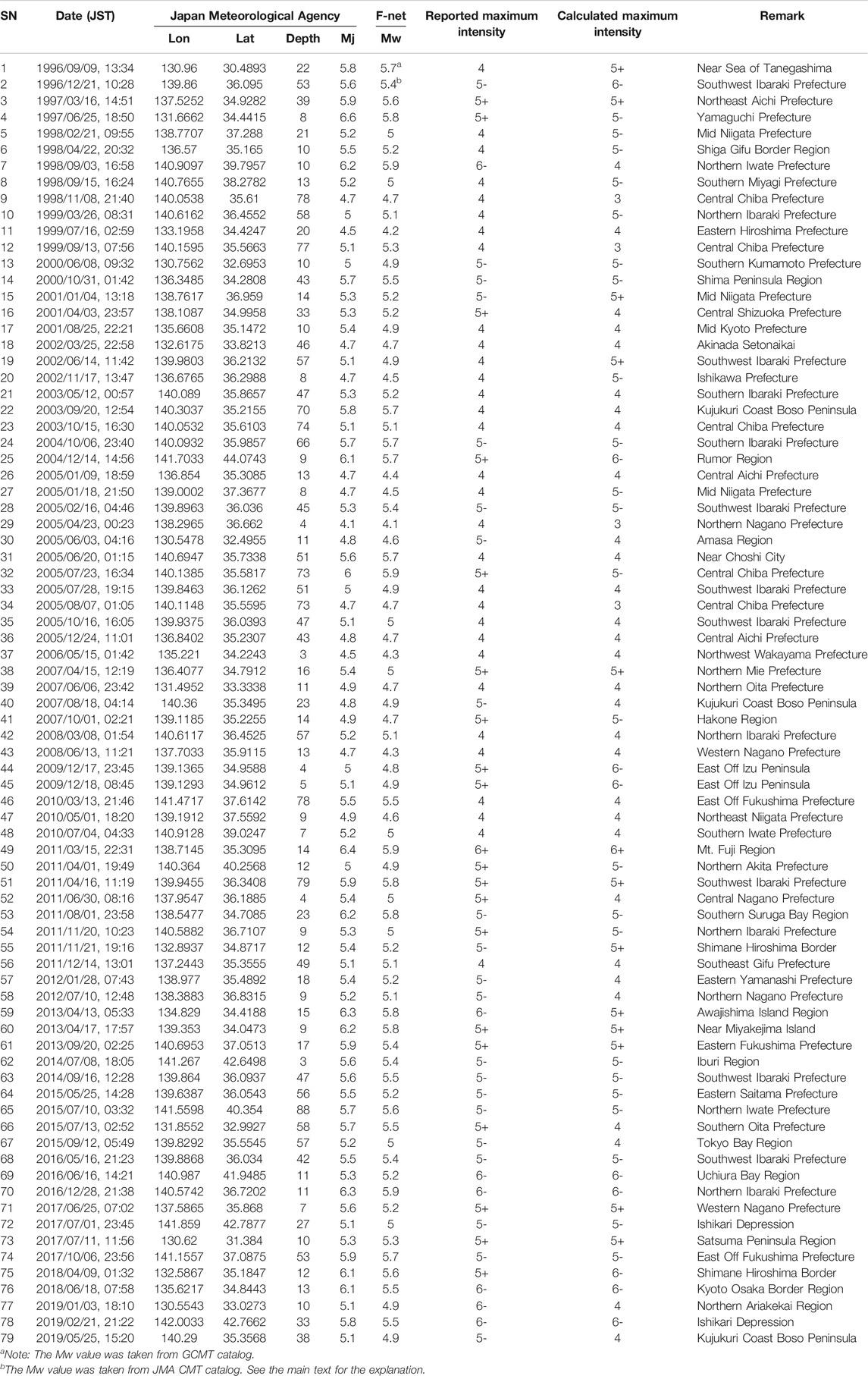
TABLE 1. List of damaging moderate magnitude earthquakes in Japan.

FIGURE 1

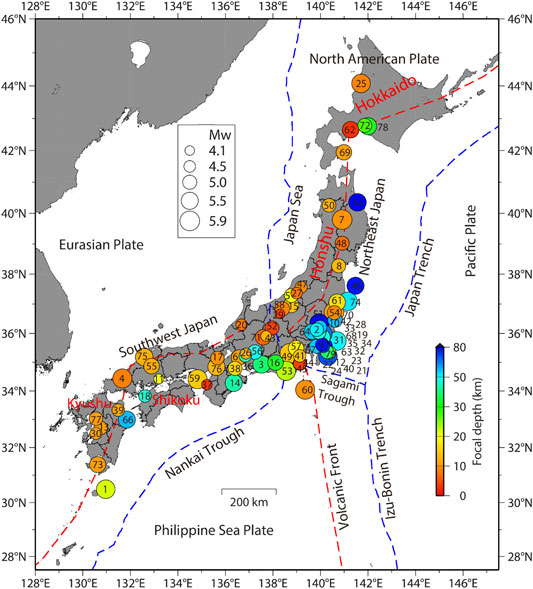
FIGURE 1. Location of the damaging moderate magnitude earthquakes (5.9 ≥ Mw) in Japan from 1996 to 2019. Circles denote the epicenters of the earthquakes. Numbers attached or close to the circles indicate the serial numbers of the events listed in Table 1.

Visual inspection of original accelerograms, velocity seismograms obtained by integrating accelerograms, and their Fourier spectra were carried out. Recordings were selected if both P- and S-onsets were present, and pre-event window of length 7 s was available. The corresponding mean acceleration of the pre-event window was reduced from the accelerograms to obtain peak ground motion parameters. Then, low cut filtering was applied at a corner frequency of 0.1 Hz for most of the recordings. However, for some recordings, the corner frequency for low-cut filtering was increased up to 0.5 Hz, based on the presence of noise. Cosine tapering was applied for a window of 5 s at both ends of the recordings. The ARS and AVRS were calculated for 5%-damping ratios using the method of Nigam and Jennings (1969). The sums of relative velocity responses and the corresponding velocity seismograms obtained by integration of filtered accelerograms give the absolute velocity responses, which were computed for each horizontal component. Finally, we calculated the vector sum of the two horizontal component absolute velocity responses and obtained the maximum value of all the time steps as the value of AVRS for each natural period.

Similarly, the ARS represents the peak vector of two horizontal component acceleration response time histories. The PGA and PGV values reported in this paper are larger ones of the PGAs and PGVs, respectively, of the two horizontal components. The definitions of PGA and PGV are different in some GMPEs, and they are defined at appropriate sections when they appear in this paper. An example plot of the acceleration and velocity seismograms is given in Figure 2 for two sites. The seismograms are discussed in the next section. The JMA instrumental intensity was computed following the procedure explained in JMA (2020b). A comparison of the JMA instrumental intensity scale with the Modified Mercalli Intensity (MMI) scale and the computation procedure of JMA instrumental intensity can also be found in Shabestari and Yamazaki (2001). Hoshiba et al. (2010) provide the relationship between the JMA intensity, JMA instrumental intensity, and MMI scale according to which JMA intensity of 4, 5L or 5−, 5U or 5+, 6L or 6−, 6U or 6+, and 7 correspond to MMI scale of 6-7, 7-8, 8-9, 9-10, 10-11, and 12, respectively.

FIGURE 2

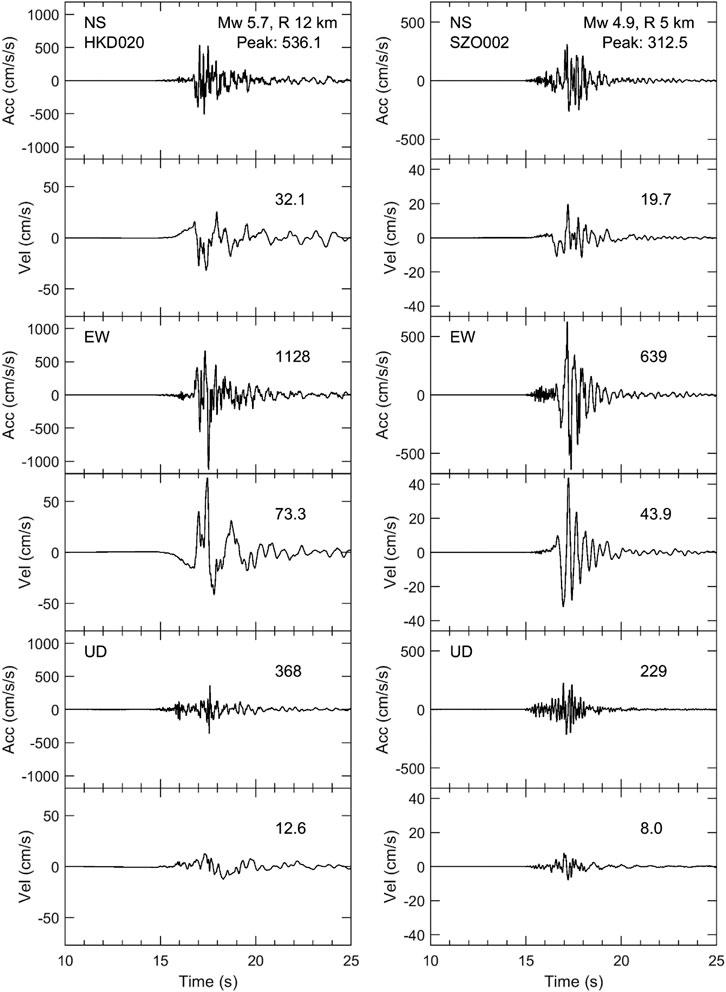
FIGURE 2. Plots of acceleration and velocity seismograms at HKD020 site for an Mw 5.7 event (left panel) and SZO002 site for an Mw 4.9 event (right panel). R denotes the hypocentral distance rounded to the closest integer. The peak values of the seismograms are written above the corresponding traces. Note the difference between the vertical scales in the left and right panels.

General Features of Strong-Motions

PGA and PGV

The PGAs and PGVs from all the earthquakes used in this study are plotted in Figures 3A,B, respectively. Figure 3A shows the PGAs (larger of two horizontal components) plotted as a function of hypocentral distance and magnitudes. The PGA values are colored by the magnitudes divided into four groups: 4.1–4.4, 4.5–4.9, 5.0–5.4, and 5.5–5.9. Out of the 79 earthquakes, 40 earthquakes had focal depths lower than 20 km. The median focal depth was about 23 km of all earthquakes. The minimum and maximum depths were approximately 3 and 88 km. The median prediction curves for Mw = 4.0, 4.5, 5.0, 5.5, and 6.0 are also shown in the figures for crustal type earthquake, focal depth of 20 km, and soil site condition using the equations in Si and Midorikawa (1999), Si and Midorikawa (2000). Similarly, the median prediction curves for interplate and intraslab earthquakes of Mw = 5.5 and 6 are drawn in the figures for two focal depths (30 km for interplate earthquake and 30 and 70 km for intraslab earthquake). The paper, Si and Midorikawa (1999), is, hereafter, referred to as SM 1999. The GMPEs in SM 1999 were constructed using events of Mw ≥ 5.8. However, the GMPEs are used here as reference GMPEs for PGA and PGV because of their widespread use in Japan. For example, the GMPEs for PGV in SM 1999 have been used by the Headquarters for Earthquake Research Promotion (HERP, 2018) in producing the national seismic hazard maps for Japan. For PGA, soil site condition means the site has Vs30 values (average S-wave velocity in the top 30 m of the soil column) lower than 620 m/s. For the PGV, the prediction curves are drawn for the Vs30 value of 300 m/s because this value is roughly the average site condition for the strong-motion stations (e.g., Kanno et al., 2006).

FIGURE 3

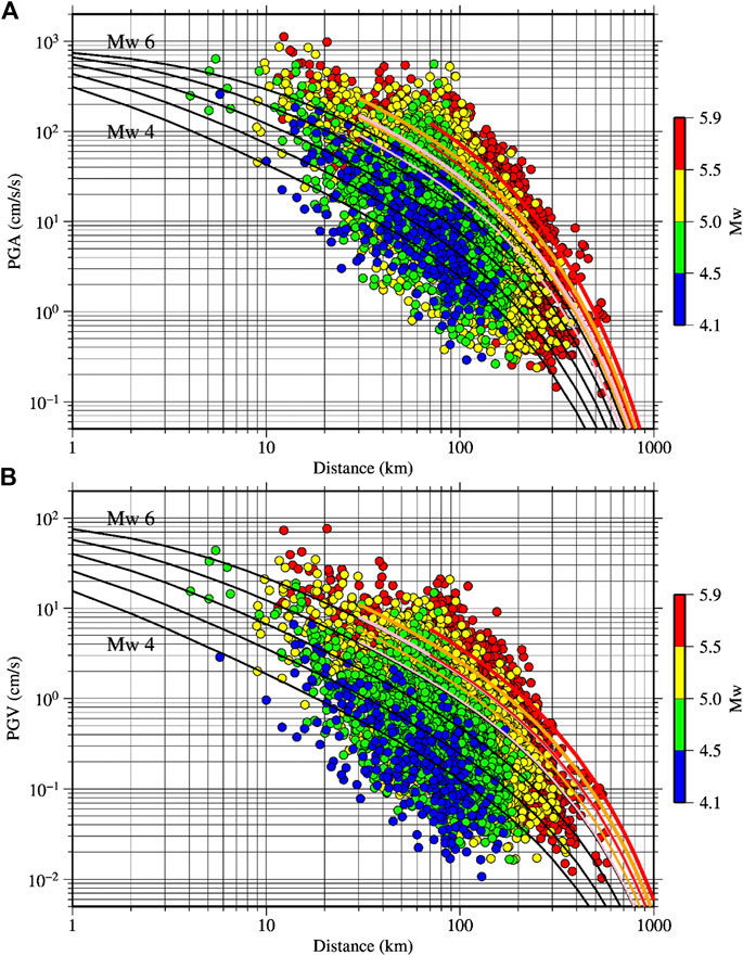
FIGURE 3. Plot of PGAs (A) and PGVs (B) as a function of hypocentral distance. The black curved lines denote the median prediction curves for crustal earthquakes for soil site conditions in (A) and Vs30 = 300 m/s in (B) for Mw = 4.0, 4.5, 5.0, 5.5, and 6.0, respectively, using the GMPEs in Si and Midorikawa (1999). The thin and thick pink (orange) lines denote the median prediction curves for interplate (intraslab) earthquakes of Mw = 5.5 and 6.0, respectively (focal depth = 30 km). Similarly, the thin and thick red lines denote the median prediction curves for intraslab earthquakes of Mw = 5.5 and 6.0, respectively, for focal depth = 70 km.

Magnitude and distance are the two most commonly employed parameters in the GMPEs. Figures 3A,B show that the PGAs and PGVs generally depend on the magnitude and the distance. The values increase with the increase of magnitudes and decrease with the increase of distances, on average. These trends are generally captured well by the prediction curves plotted in the figures. However, a significant proportion of the data between the magnitude groups overlap. The amplitude and frequency content of ground motions are strongly modified by the local site conditions, propagation path, and source factors such as focal mechanisms, stress drops, rupture directivity effects and so on (e.g., Campbell, 2003). To see the variation of the PGA and PGV values with respect to the magnitude, focal depth, and site condition clearly, the PGA and PGVs are shown repeatedly in Figure 4 by selecting the data over 100 cm/s². The log-scales used in Figure 3 for the horizontal axes are changed to linear scales, and the ranges of vertical and horizontal scales are narrowed down in Figure 4. Figures 4A,B show that the PGA values for the deeper events are larger than those for the shallower events. In Figure 4C, PGVs are plotted as a function of distance, and the values are colored by magnitudes. Even though the largest PGVs seen over wider distance bins are from large magnitude events, the PGVs from three magnitude bins (4.5–4.9, 5.0–5.4, 5.5–5.9) noticeably overlap within 10–30 km. The PGVs are color-coded by Vs30 values in Figure 4D. The PGV values at sites where Vs30 were not available are shown by open circles. The open circle data are from the K-NET stations. K-NET stations had PS-loggings down to the depth of 20 m. In this study, the Vs30 values for the K-NET stations were obtained using the correlation formula between the Vs20 and Vs30 in Kanno et al. (2006) for the sites where Vs20 was available. But many stations had PS-loggings down to the depth of 10 m. The open circles in Figure 4D are the sites lacking measured Vs20. It can be seen in Figure 4D that the PGVs are generally larger for sites with smaller Vs30 values. These figures showed that the PGAs and PGVs are generally larger for the deeper earthquakes and at sites with lower Vs30 values.

FIGURE 4

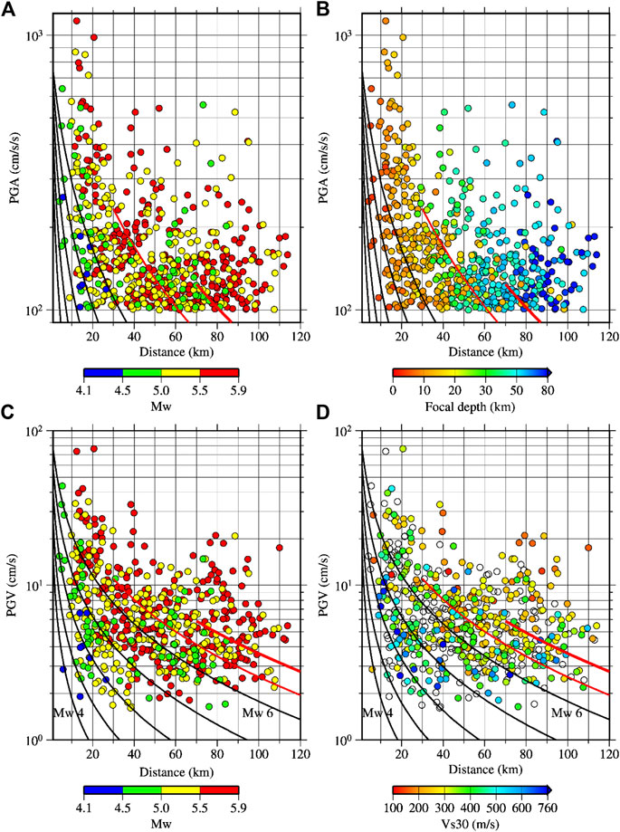
FIGURE 4. (A,B): same plot as in Figure 3A, but the PGA values smaller than 100 cm/s/s are not shown, and the hypocentral distance is limited to 120 km. The data in (A) are color-coded by magnitude while data in b by focal depths. (C,D): similar to (A,B), but for the PGVs. The data are color-coded by magnitudes in (C) and by Vs30 in (D). Open circles show data lacking Vs30 values. The black curved lines denote the prediction curves in the same order, as plotted in Figure 3. The red thin and thick lines denote the median prediction curves for intraslab earthquakes of focal depths 30 and 70 km, respectively, for Mw = 6. The prediction curves were obtained using the GMPEs in Si and Midorikawa (1999).

Here I discuss the plots of residuals for PGAs and PGVs against the different variables used in the GMPEs and against the predicted and observed values. The residuals in base-10 log-scale are plotted in Figure 5 for the PGAs from hypocentral distances smaller than 200 km. The residuals were grouped into different bins, and the binned mean values with plus-minus one standard deviation are also indicated in the figure. The binned mean residuals against the Mw values plotted in Figure 5A are positive, and the values decrease with the increase of magnitude. The mean values ranged between approximately 0.06 and 0.16. Similarly, the residuals against the hypocentral distance are plotted in Figure 5B. The plot shows that the binned mean residuals gradually decrease from short to long distances. In the construction of GMPEs in SM 1999, fault distance was used as a measure of source-to-site distance. I used the hypocentral distance as a measure of distance because the fault models of the events were not available except for few events. A mismatch between the fault distance and hypocentral distance may have resulted in the relatively larger residual values at the short distances. However, most of the recordings were from Mw values smaller than 5.5 for data points at short distances, and hence the difference between the fault and hypocentral distance may be small (see the Supplementary Material for the magnitude versus distance distribution of data). The residuals against the focal depth plotted in Figure 5C do not show a definite trend. The binned mean residuals plotted against the Vs30 values in Figure 5D show positive values for Vs30 values smaller than 600 m/s. For larger Vs30 values, the binned means are negative. The residuals against the predicted values and observed values are plotted in Figures 5E,F, respectively. The binned mean residuals for predicted PGAs >50 cm/s² are relatively larger. The residuals plotted against the observed values show a linear trend in Figure 5F. The binned mean residuals for the observed PGAs >100 cm/s² are larger than 0.6, which is larger than twice the standard deviation reported in SM 1999. The amount of data at small distances is fewer and the use of hypocentral distance is different from the fault distance used in the GMPEs. Therefore, the absolute value of residuals at short distances may not be accurate. However, the systematic difference of residual values between the soil and rock sites separated by Vs30 value of 620 m/s may indicate that the classification of sites into soil and rock based on the Vs30 value of 620 m/s may not be sufficient.

FIGURE 5

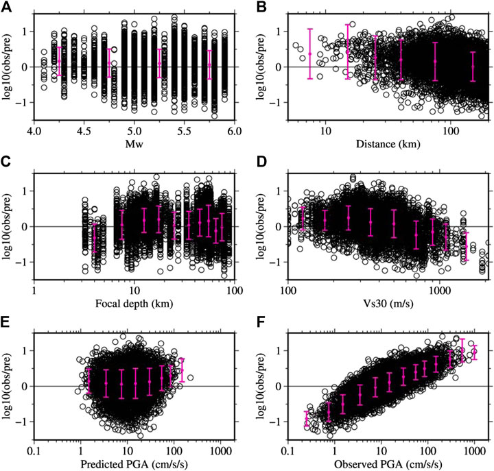
FIGURE 5. Plots of residuals for PGA data plotted in Figure 3A for hypocentral distances smaller than 200 km. The (A–F) show the distribution of residuals against the Mw, hypocentral distance, focal depth, Vs30, predicted PGA, and observed PGA, respectively. The vertical bars denote the mean values with plus-minus one standard deviation of the binned residuals.

The distributions of residuals for PGVs against the Mw, hypocentral distance, focal depth, Vs30, predicted PGV, and observed PGV are shown in Figures 6A–F, respectively. Different from the results for PGAs discussed above, the binned mean residuals tended to be lower for the PGVs. A gentle trend with Vs30 is seen; this is different from that for the PGAs, and may be due to that the Vs30 was used as continuous variable in the GMPEs for PGVs than just soil and rock sites for the PGAs. The binned mean residuals at small distances were relatively larger than at longer distances. The binned mean residuals for the observed PGVs > than 10 cm/s were larger than twice the standard deviation for PGV in SM 1999.

FIGURE 6

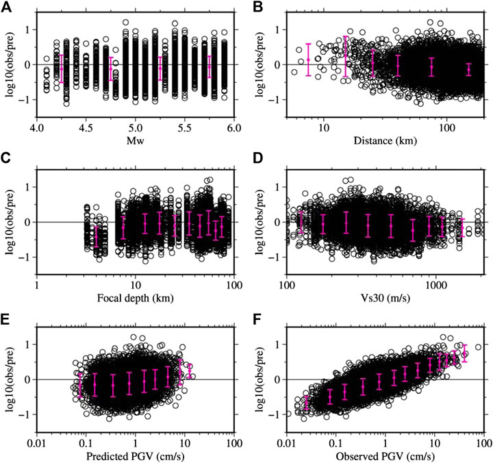
FIGURE 6. Plots of residuals for PGV data plotted in Figure 3B for hypocentral distances smaller than 200 km. The (A–F) show the distribution of residuals against the Mw, hypocentral distance, focal depth, Vs30, predicted PGA, and observed PGA, respectively. The vertical bars denote the mean values with plus-minus one standard deviation of the binned residuals.

The largest PGA was approximately 1,128 cm/s², which was recorded at HKD020 (see Figure 2) during an Mw 5.7 event that occurred on December 14, 2004, at 14:56 JST in Rumoi, Hokkaido (see Figure 1 for the location of the epicenter, Event no. 25). The maximum value of the PGV for the event was about 73 cm/s, which was also recorded at HKD020 (see Figure 2). The largest PGV of approximately 76 cm/s was observed at the SZO011 site during an Mw 5.9 event (Event no. 49, see Figure 1 for the event location); the observed PGA was ∼981 cm/s² at the site during the event. The instrumental intensities at the HKD020 and SZO011 sites were approximately 5.9 and 6.4, respectively. These values translate to 6− and 6+ intensities in the conventional JMA intensity scale and are identical to the reported maximum intensities for the two earthquakes (see Table 1).

Here I briefly discuss the mechanisms for the large PGA and PGV at the HKD020 site during the Mw 5.7, Hokkaido Rumoi earthquake, based on available literature. The site’s location, the epicenter of the event, and the F-net focal mechanism solution are given in a Supplementary Material. The site had S-wave velocity profiles known down to the depth of 10 m based on PS-logging, and the Vs10 was approximately 398 m/s. Based on empirical H/V spectral analysis and theoretical amplification models based on available shallow and deep velocity models, Maeda and Sasatani (2009) reported that the site amplification was not sufficient to explain the large PGA, PGV, and pseudo-velocity response spectrum exceeding 100 cm/s at frequencies of about 0.5–1.5 Hz at the site. Using empirical Green's function method, Maeda and Sasatani (2009) constructed a source model for the earthquake. Based on the used parameters and agreement between the observed and synthetic waveforms, they concluded that the earthquake was a typical crustal earthquake, and the large PGA and PGV were due to the source effect (close to the strong motion generation area and forward rupture directivity). Later on, Sato et al. (2013) conducted detailed geophysical borehole loggings and estimated input motions at a depth of 41 m that corresponded to Vs layer of 700 m/s. They showed that input PGA was approximately 50% smaller than the surface PGA, but the PGV was only around 20% smaller. They showed that 3–13 Hz ground motions were amplified by the soil layers above, while higher than 13 Hz were reduced by nonlinearity. I examined the PGV ratios at different frequency bands between the NS and EW components and found that the difference was the largest between 0.5 and 3 Hz (larger than a factor of two, 56 cm/s vs. 21 cm/s, between the two components). I found that the contribution to the PGV by the frequency band between 3 and 13 Hz was small, which is generally an expected result because the PGV better represents the intermediate period ground motions. On the other hand, the PGA of this frequency band was approximately 644 cm/s², and for the lower frequencies between 0.5 and 3 Hz, it was 560 cm/s², suggesting that the PGA was governed by broad frequency ranges between about 0.3 and 13 Hz. As shown in Figure 2, the EW-component had the PGV approximately 2.3 times the NS-component (73 cm/s versus 32 cm/s approximately). The site was located up-dip in the rupture propagation direction of a reverse fault, and the EW-component roughly coincides with the fault-normal component. Thus, the geometry between the fault and site and the large amplitude difference between the two horizontal components suggested that the cause of the large PGA and PGV was most probably the forward rupture directivity effect (Sommerville et al., 1997), and the aggravation by site amplification including the nonlinear one (e.g., Sato et al., 2013; Garini et al., 2017; Dhakal et al., 2019).

Even though the dominating values of PGAs and PGVs were mostly from the large magnitude events, the color scale in Figures 3, 4 shows that relatively large PGAs and PGVs are possible from smaller magnitude events (Mw < 5) at short distances (<7 km). The PGAs and PGVs at these small distances were between 170 and 639 cm/s², and 3–44 cm/s, respectively; the largest PGA and PGV were from an Mw 4.9 event recorded at the SZO002 site. Though it is beyond the scope of this paper to discuss each event, the above-mentioned Mw 4.9 event is briefly discussed here. The event occurred on December 18, 2009, at 08:45 JST (Event no. 45 located near the west end of the Sagami Trough; see Figure 1 for the location of the event and Table 1 for the other information about the event). The acceleration and velocity seismograms at the SZO002 site are plotted in Figure 2 (right panels). The S-wave profile at the site was available up to 12 m, and the Vs10 at the site was 232 m/s. Figure 2B shows that the PGV on the EW-component is approximately 2.2 times the PGV on the NS-component. Available literature (HERP, 2010) did not uniquely identify the causative fault’s geometry for this earthquake. The earthquake’s focal mechanism based on F-net, NIED, moment tensor solution is given in a Supplementary Material. The mechanisms suggest steeply dipping roughly east-west fault or north-south strike-slip fault. The site was located roughly west of the epicenter. The strike-slip mechanism can produce large amplitude normal to the strike, in this case the EW-component at the SZO002 site. Based on the F-net solution and the observed PGVs on the two components, a strong source radiation effect can be suspected at the site. The reported maximum intensity for this event was 5+. The computed instrumental intensity in this study is 5.65, which translates to 6- based on the intensity class divisions (5.0–5.4: 5+; 5.5–5.9: 6-) (JMA 2020b). In Figure 3, it can be seen that the PGAs and PGVs within the distance of 7 km are larger than those indicated by the median prediction curves for their magnitude values.

Instrumental Intensity

The instrumental intensities for all the events analyzed in this study are plotted in Figure 7A. The values are color-coded by the magnitudes. Median prediction curves for the instrumental intensities are also plotted based on the equations in Morikawa and Fujiwara (2013) for crustal earthquakes (Mw = 4, 4.5, 5, 5.5, and 6), interplate earthquakes (Mw = 5.5 and 6), and intraslab earthquakes (Mw = 5.5 and 6). Hereafter, the paper, Morikawa and Fujiwara (2013), is referred to as MF 2013. Similar to the PGAs and PGVs, the intensities also are larger for larger magnitudes, on average, and the prediction curves clearly capture the trends. Instrumental intensities larger than five were observed from events having Mw < 5 at short distances and up to approximately 100 km. An instrumental intensity of over five was recorded at the TCG009 site located at the hypocentral distance of approximately 90 km during an Mw 5.4 event; the focal depth of the event was 53 km (Event no. 2, southwest Ibaraki Prefecture earthquake, see Table 1; Figure 1 for event location). The Vs30 value at the TCG009 site was approximately 247 m/s. However, instrumental intestines of 5 and over were mostly within smaller than 50 km. At short distances of 10–20 km, larger intensity values were most probably governed by magnitudes and rupture directivity effects for these moderate magnitude earthquakes as discussed in the previous section, while at the longer distances, the intensity values near five were observed at sites having lower Vs30 values.

FIGURE 7

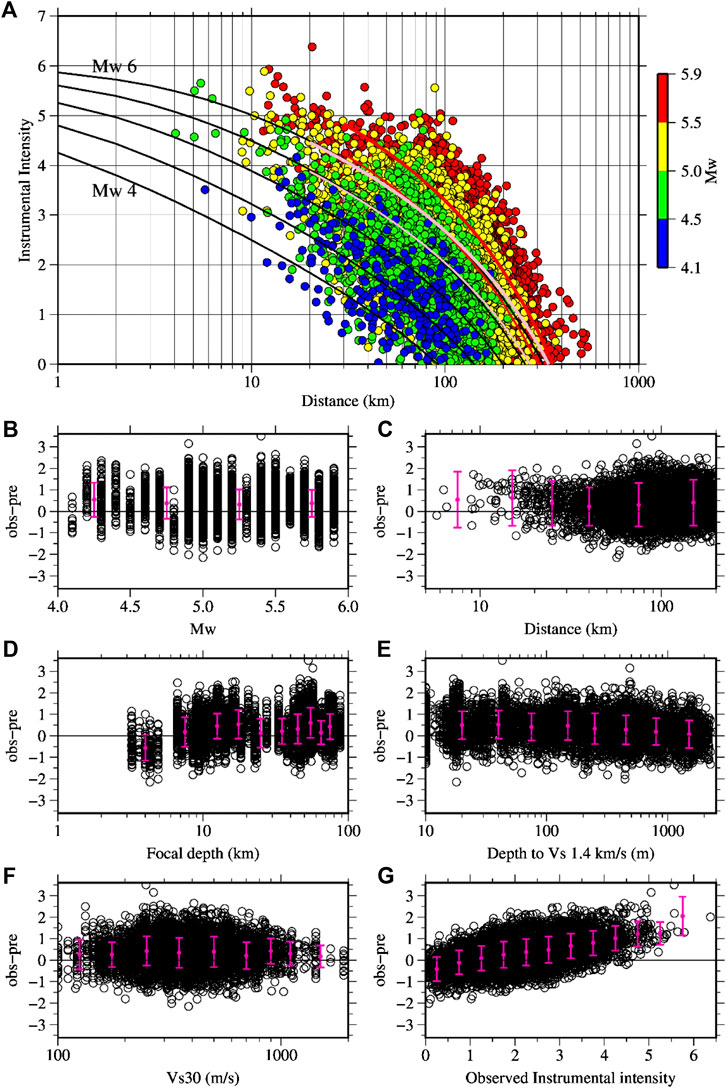
FIGURE 7. (A) JMA instrumental intensities for the same set of data plotted in Figure 3. The black lines denote the median prediction curves for crustal earthquakes of Mw = 4, 4.5, 5, 5.5, and 6, respectively, using the GMPEs in Morikawa and Fujiwara (2013). The thin and thick pink (red) lines denote the median prediction curves for Mw = 5.5 and 6, respectively, for the interplate (intraslab) earthquakes. (B–G) show the distribution of residuals against the Mw, hypocentral distance, focal depth, depth to Vs 1.4 km/s, Vs30, and observed instrumental intensity, respectively. The vertical bars denote the mean values with plus-minus one standard deviation of the binned residuals.

Figures 7B,G shows the plots of residuals (observed instrumental intensity–predicted instrumental intensity) based on the GMPEs for instrumental intensity in MF 2013. The binned mean residuals against the Mw values and hypocentral distances are positive, and their trends are similar to those plotted in Figures 5A,B for the residuals for PGAs. The binned means are relatively larger for smaller magnitude events and at short distances. In MF 2013, two different parameters were used for site corrections. They are the depth to Vs 1.4 km/s for the effect of deep sediments and Vs30 for the effect of shallow sediments. The depths to Vs 1.4 km/s were taken from the J-SHIS (Japan Seismic Hazard Information Station) subsurface velocity model (Fujiwara et al., 2009) (see the Data Availability Statements). The binned mean residuals decrease with the increase of sediment thickness (Figure 7E), and the binned mean residuals do not show a definite trend with the Vs30 (Figure 7F). The binned mean residuals plotted against the observed instrumental intensities in Figure 7G show that the binned mean residual values range approximately between 0.5 and 2 for observed intensities larger than 4. Most probably, the damages from these small to moderate earthquakes were related to the large ground motions, which are underpredicted considerably by the GMPEs employed in the present study.

AVRS

The AVRS at the periods of 1.6, 2.0, 3.0, and 4.0 s are plotted as a function of hypocentral distance and colored by magnitudes in Figure 8. As briefly described in the introduction section, long-period ground motion intensities (LPGMIs) are calculated from the AVRS in the period band of 1.6–7.8 s. The maximum value determines the level of intensity. The intensity levels are as follows: class 1 (5–15 cm/s), class 2 (>15–50 cm/s), class 3 (>50–100 cm/s), and class 4 (>100 cm/s). These intensity levels are indicated in Figure 8. Out of the 79 earthquakes, 47 earthquakes produced LPGMI of 1 or over, totaling 489 recordings. The dominant peak period was 1.6 s within the band of 1.6–7.8 s from 346 recordings. The number of recordings with the dominant peak period of 1.8 s was 59, the second-largest number. Similarly, the number of recordings with dominant peak periods between 2 and 2.8 s was 62, between 3 and 3.8 s was 13, and between 4 and 5 s was 9. The dominant peak periods >3 s were mostly from the Kanto basin area and were not from shallow events, but with focal depths between 20 and 40 km and magnitudes between 5.4 and 5.7. In Figure 1, it can be seen that most of the events have larger focal depths in the Kanto area, north of the Sagami Trough. However, the maximum intensity from these longer periods was 2. During the June 18, 2018, 07:58, North Osaka earthquake, LPGMI of level 2 was observed at ten sites, and the peak periods from the band of 1.6–7.8 s were mostly 1.6 s. It can be clearly seen in Figure 8 that the number of recordings with intensity 2 is only two at the period of 4 s. Also, from the plots in Figure 8, it may be inferred that the moderate earthquakes are of not serious concern at distances beyond 200 km. The distribution of peak spectral periods from the period band of 1–10 s against the Mw, hypocentral distance, focal depth and depth to Vs 1.4 km/s are provided in the Supplementary Material. In the Supplementary Material, the peak spectral periods are shown only for the records for which the maximum AVRS was >1 cm/s in the period band of 1–10 s. The peak periods increased generally with the increase of magnitude, hypocentral distance, and sediment thickness, while they decreased with the increase of focal depths. However, the peak periods scattered largely suggesting that multiple parameters can influence the spectral values and hence the peak periods.

FIGURE 8

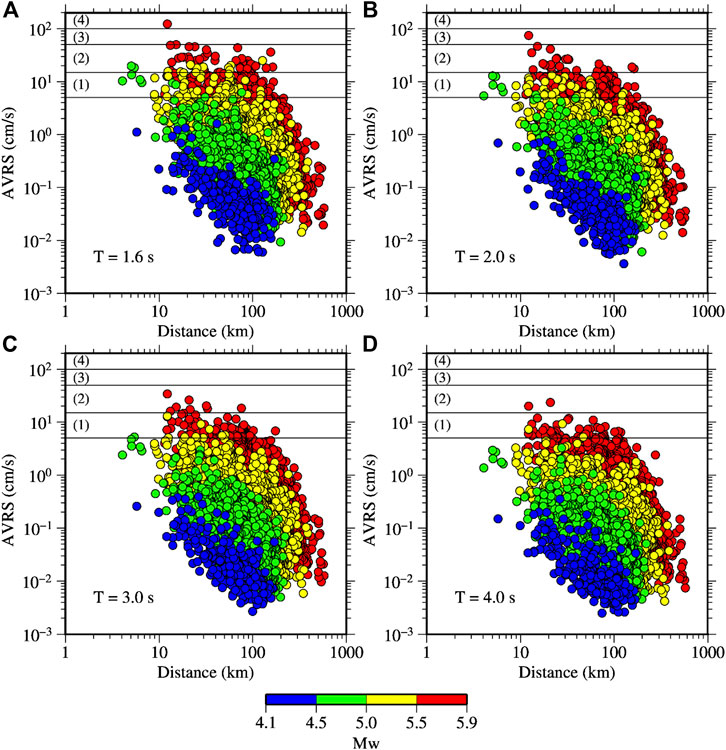
FIGURE 8. Absolute velocity response spectra (AVRS) at the periods of 1.6, 2.0, 3.0, and 4.0 s plotted against the hypocentral distance in A, B, C, D, respectively. The horizontal lines across the AVRS of 5, 15, 50, and 100 cm/s mark the threshold values for JMA long‐period ground motion intensities of 1, 2, 3, and 4, respectively.

North Osaka Earthquake

Strong-Motions

The epicenter of the 2018 North Osaka earthquake is shown in Figures 9A,B. The larger values of the two horizontal components’ PGAs and PGVs observed at small distances are depicted along with the site codes in Figure 9B. Within an epicentral distance of 20 km, ten strong-motion stations of K-NET and KiK-net recorded the ground motions. Out of the ten stations, eight stations recorded PGAs >200 cm/s² and PGVs >15 cm/s. The maximum PGA and PGV were approximately 794 cm/s² and 40 cm/s, respectively, recorded at an epicentral distance of approximately 2.7 km at the same site (OSK002, Takatsuki). It was shown by several studies that the North Osaka earthquake occurred on two different faults closely separated in space almost simultaneously (Kato and Ueda, 2019; Hallo et al., 2019). As shown in Figure 9B, one of the events was a reverse fault (F1 in the figure), and the other was a strike-slip fault (F2 in the figure). The start of slips on fault F2 was about 0.3 s after the start of slips on the fault F1 (Kato and Ueda, 2019). The plots of aftershocks and fault models by Kato and Ueda (2019) (see Figure 2 in Kato and Ueda, 2019) showed that the OSK002 site was located on the footwall of the north-south striking east-dipping reverse fault, and in the direction of the rupture propagation (see Figure 9B for the site location). The large PGV was observed on the EW-component, which is roughly perpendicular to the strike of the reverse fault. This observation also supports that the forward rupture directivity contributed to the generation of the large PGV on the EW-component. Figure 10 shows a comparison of the observed PGAs and PGVs with the median prediction curves for three different GMPEs: Figures 10A,B SM 1999, Figures 10C,DKanno et al. (2006), and Figures 10E,F MF 2013. Hereafter, the equations in Kanno et al. (2006) are abbreviated as KN 2006. The Mw value for the North Osaka earthquake estimated by Kato and Ueda (2019) and Hallo et al. (2019) was 5.6. In the present study, I used the F-net (NIED) Mw value of 5.5 for the median prediction curve for uniformity with the Mw values used in this paper for other earthquakes and in KN2006 and MF 2013. However, the mean errors using the Mw value of 5.6 are also plotted in Figure 11 for the comparison. The observed values are colored to the Vs30 values in Figures 10A–D, while the values in Figures 10E,F are colored to the depth of Vs layer of 1.4 km/s. This is because SM 1999 and KN2006 used Vs30 values for site corrections, while the MF 2013 used both the Vs30 and depth of Vs layer of 1.4 km/s. It is expected that the color scales provide a general view of the site profiles.

FIGURE 9

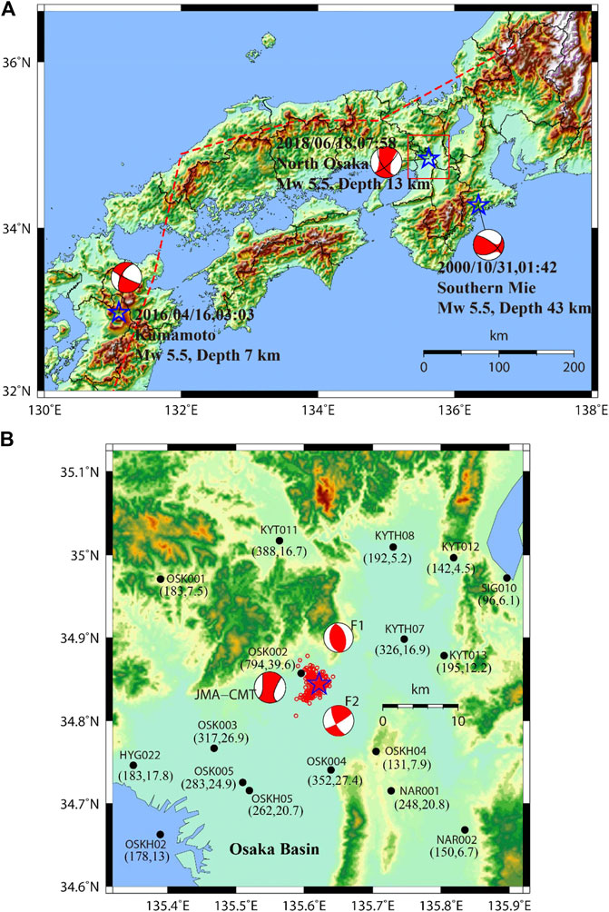
FIGURE 9. (A) Stars denote epicenters of three Mw 5.5 earthquakes in North Osaka, Southern Mie, and Aso Kumamoto regions, as depicted in the figure. The rectangle around the epicenter is the enlarged area in (B). The red dashed line represents the volcanic front. The F1 and F2 written near the focal mechanism plots in (B) are the double couple mechanisms proposed by Kato and Ueda (2019) for the two subevents of the North Osaka mainshock. The small red circles denote the aftershocks having JMA magnitude >1 recorded within 24 h after the mainshock. The black filled circles represent the strong-motion observation stations. The site codes and the recorded larger PGA and PGV of the two horizontal components are given within parenthesis near the observation stations.

FIGURE 10

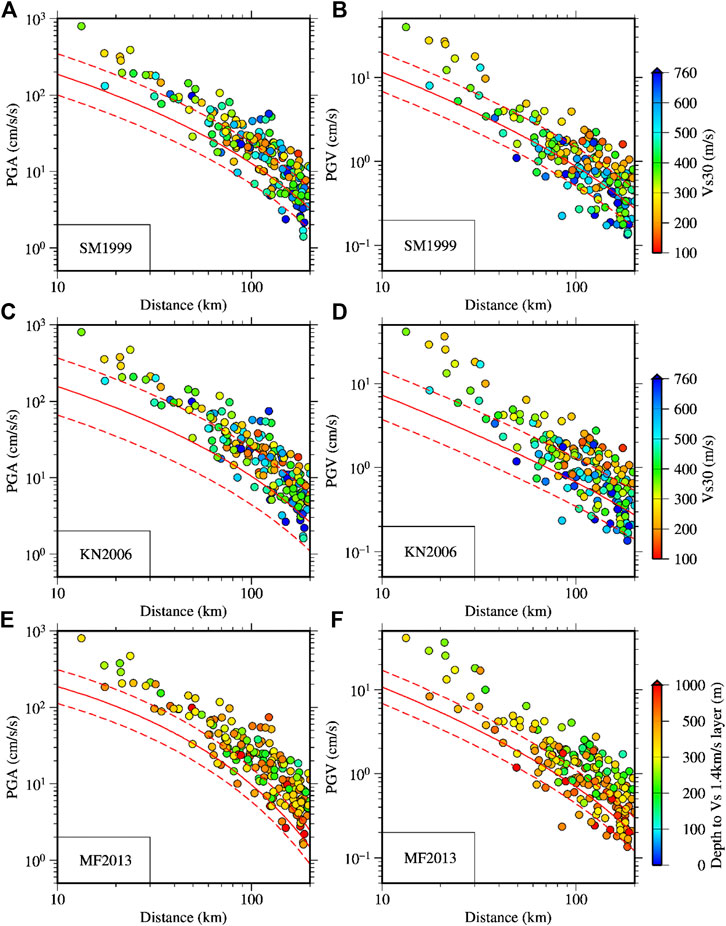
FIGURE 10. Comparison of the observed PGAs and PGVs during the Mw 5.5 North Osaka earthquake with the ground motion prediction curves. The horizontal axes denote the hypocentral distance. The data points in panels (A–D) are color-coded by Vs30 values while the data in (E,F) are by depth to Vs 1.4 km/s. The used prediction equations are indicated in each panel by alphanumeric codes. The codes SM 199, KN 2006, and MF 2013 mean the prediction equations in Si and Midorikawa (1999), Kanno et al. (2006), and Morikawa and Fujiwara (2013), respectively.

FIGURE 11

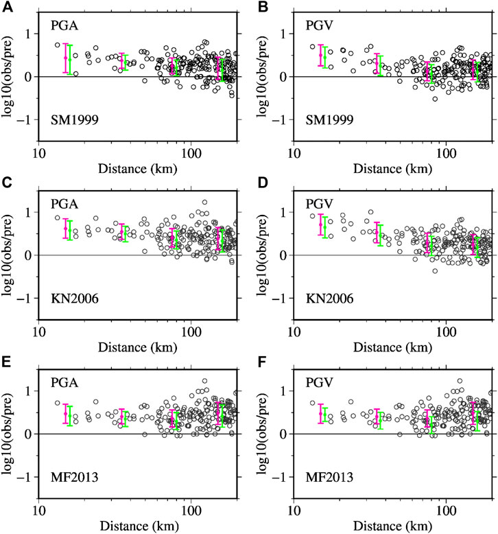
FIGURE 11. Plots of residuals as a function of hypocentral distance after the site corrections for the data plotted in Figure 10 for the PGAs and PGVs. The figure parts A-F correspond to the figure parts in Figure 10. The residual values shown in the plots were obtained for the Mw value of 5.5. The magenta-colored vertical bars represent the error bars for binned data with mean error and plus‐minus one standard deviation. The green‐colored vertical bars show the error bars for comparison for the Mw value of 5.6.

In Figure 10, it can be seen that the PGAs and PGVs at distances smaller than about 50 and 40 km, respectively, are larger than the median values on average. Figure 11 shows the plots of residuals after the site corrections. The binned mean errors for two magnitude values (Mw = 5.5 and 5.6) are also plotted as a function of distance. The mean errors suggest a distance dependence of the residuals for PGAs and PGVs for the SM 1999 and KN 2006. On the other hand, the mean residuals are generally uniformly distributed for the MF 2013. The mean residuals give that the PGA data are larger by a factor of about 2.7, 2.3, and 1.8 than the values from the median prediction curve at distances smaller than 20 km, between 20 and 50 km, and between 50 and 100 km, respectively, on average, for the SM 1999.

Similarly, the PGV data are larger by a factor of about 3.2, 2.0, and 1.3 at the above distance ranges, respectively, for the SM 1999. The results for the KN2006 are also similar: the PGA data are larger by factors of about 4.2, 3.5, and 2.6, while the PGV data are larger by factors of about 5, 3.3, and 1.9. The results for the MF 2013 are also similar: for the PGA, the data are larger by factors of about 3, 2.5, and 2.3, respectively, and for the PGV, the data are larger by factors of about 3.2, 2.3, and 1.9, respectively. The binned mean errors for the case of Mw = 5.6 are slightly smaller than the values for the case of Mw = 5.5. Based on the above results, it may be said that SM 1999, which has been used in the seismic hazard estimation for Japan by HERP (2018), gives the smallest error for the North Osaka earthquake. In general, all the equations used underpredicted the PGAs and PGVs for the North Osaka earthquake.

Figure 12 shows the residual plots for acceleration response spectra at the periods of 0.1, 0.5, 1, 2, 5, and 7 s after the site corrections, using the prediction equations in MF 2013. At periods up to 2 s, the results are similar to those discussed above for PGA and PGV. However, at the periods of 5 and 7 s, the residuals were generally within the expected range of errors at longer distances, while the data were noticeably underpredicted at distances smaller than about 40 km. The plots of the observed data as a function of distance for the above periods are shown in a Supplementary Material.

FIGURE 12

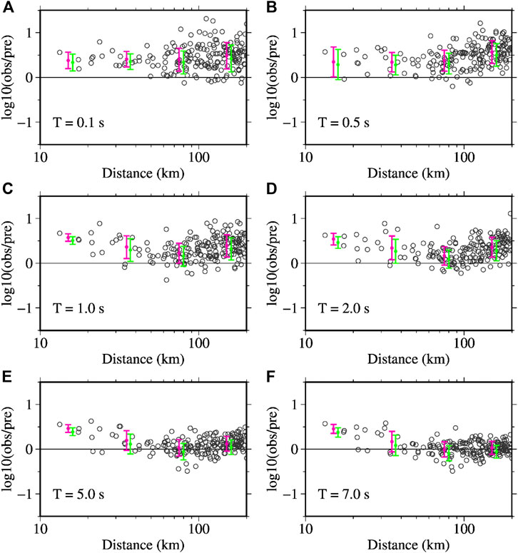
FIGURE 12. Plots of residuals as a function of hypocentral distance after the site corrections for the acceleration response spectra (ARS) at the periods of 0.1, 0.5, 1, 2, 5, and 7 s in panels, A-F, respectively, using the prediction equations in Morikawa and Fujiwara (2013). The residual values shown in the plots were obtained for the Mw value of 5.5. The magenta‐colored vertical bars denote the error bars for binned data with mean error and plus‐minus one standard deviation. The green‐colored vertical bars show the error bars for comparison for the Mw value of 5.6. See the supplementary file for the plots of ARS values as a function of hypocentral distance.

Comparison With Other Events

Here, the PGAs and PGVs from the North Osaka earthquake are compared with those from the other two earthquakes of identical Mw values of 5.5 but differing focal depths. One of the earthquakes occurred as a shallow crustal event beneath the northeast Kumamoto Prefecture at a focal depth of 7 km on April 16, 2016, at 03:03 local time, and the other as an intraslab earthquake in the subducting Philippine Sea Plate at the focal depth of 43 km on October 31, 2000, at 01:42 local time (Event no. 14 in Table 1). The first event may be an aftershock of the Mw 7.1 Kumamoto earthquake (e.g., Hashimoto et al., 2017). This Mw 5.5 Kumamoto event is, however, not available in the list of events in Table 1 because this event was not listed in the list of damaging events. If any damage occurred from this event, the reports were perhaps combined with the mainshock event, which occurred less than two hours before this small event. The epicenters of the earthquakes used here are depicted in Figure 9A. In Figures 13A,B, the PGAs and PGVs, after adjusting for the site corrections, are plotted, respectively, as a function of distance for the North Osaka and northeast Kumamoto earthquakes, together with the prediction curves by MF 2013. It can be seen that the data for the shallow focus northeast Kumamoto earthquake are generally described well by the prediction curves for both PGAs and PGVs. On the other hand, the difference is considerable between the observed data and the median prediction curves for the North Osaka Earthquake, as discussed previously.

FIGURE 13

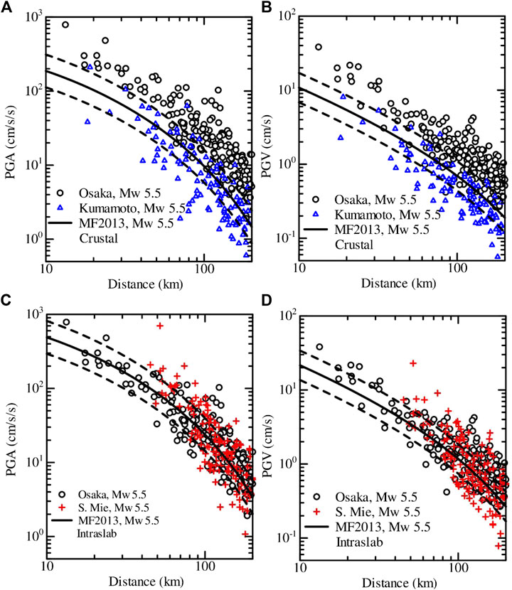
FIGURE 13. Comparison of the PGAs and PGVs between three events having identical Mw value of 5.5 (F‐net, NIED). A-B: between the North Osaka and northeast Kumamoto Prefecture earthquakes. C-D: between the North Osaka and southern Mie Prefecture earthquakes. The horizontal axes denote the hypocentral distance. The circles, cross marks, and triangles denote the adjusted values by site corrections using equations in Morikawa and Fujiwara (2013) for the events indicated in each panel. See Figure 9(a) for the location of the events. See the text for further explanation.

Similarly, the data from the relatively deep focus (43 km) southern Mie Prefecture earthquake and the North Osaka earthquake are plotted together for PGAs in Figure 13C and for PGVs in Figure 13D, after adjusting for the site corrections. The prediction curves drawn in Figures 13C,D are for the intraslab earthquake category in MF 2013. It can be seen that the data for the southern Mie Prefecture earthquake and the North Osaka earthquakes are generally described well by the prediction curves.

It has been known that the static stress drop generally increases with the increase of focal depths for inland crustal earthquakes (e.g., Asano and Iwata 2011), and the stress drop is larger for the intraslab earthquakes (e.g., Morikawa and Sasatani, 2004). The difference in the focal depth between the North Osaka earthquake (13 km) and the Kumamoto earthquake (7 km) is not large. This difference may only partially explain the observed difference of the PGAs and PGVs between the two earthquakes. The mean event residual computed from the data within 200 km for the northeast Kumamoto earthquake after the site corrections was approximately −0.14 for PGA in the base-10 log-scale. Although the error is within the range of estimation errors, the negative value suggests that the median prediction curve tends to overestimate the northeast Kumamoto earthquake data. This observation is in line with that the aftershocks tend to have a lower level of stress drops than the mainshocks, at least for smaller aftershocks (e.g., Nakano et al., 2015; Bindi et al., 2018), resulting in lower high-frequency ground motions. In the volcanic region in Japan, it has been shown that the low Q mantle wedge can cause considerable attenuation of short-period ground motions in the back-arc (BA) regions than in the fore-arc (FA) regions (Kanno et al., 2006; Morikawa and Fujiwara 2013; Dhakal et al., 2010). The PGAs and PGVs for the northeast Kumamoto earthquake were grouped into the FA, and BA regions separated by the volcanic-front and are shown in Figure 14. The plots do not indicate a noticeable effect of the low Q mantle wedge. The observed general similarities of the PGAs and PGVs between the north Osaka and the relatively deep focus southern Mie Prefecture earthquake mentioned above also augmented the possibility that the North Osaka earthquake was a higher stress drop event. Thus, one of the reasons for the discrepancy between the observed values and the prediction curves for the moderate events discussed here is likely due to the variability of stress drops among the events (e.g., Baltay et al., 2013; Oth et al., 2017; Bindi et al., 2018). It is also likely that the almost concurrent fault movements on two closely located faults with different orientations but with comparable magnitudes caused the larger ground motions during the North Osaka earthquake.

FIGURE 14

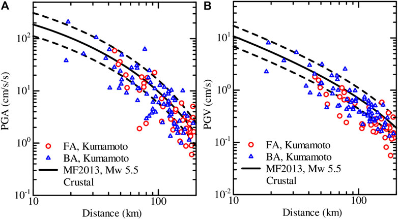
FIGURE 14. Same as in Figures 13A,B for the northeast Kumamoto earthquake, but here the data are grouped into the fore-arc (FA) and back-arc (BA) regions. See the text for further explanation.

Conclusion

PGA, PGV, JMA instrumental intensity and AVRS from 79 damaging moderate magnitude earthquakes were analyzed and presented. It was found that the focal depth and site Vs30 values were significant contributing factors for large values at longer hypocentral distances. At smaller distances (<30 km), considerable overlap was seen between the differing magnitudes producing similar PGA, PGV, and intensities. This overlap exists due to the contributions of both sources and sites. Based on the available literature and the analyzed data, source effects, mostly forward rupture directivity effect was found to produce the large velocity pulses even for the Mw 4 class events. Moderate earthquakes of Mw 4 class can generate an instrumental intensity of 4 or larger at short distances and up to about 80 km from the hypocenter of deeper earthquakes of focal depths 50–60 km. The instrumental intensities were smaller than 4 at distances > about 120 km from these moderate magnitude events. The analysis of residuals for the PGA, PGV, and instrumental intensities based on the GMPEs suggested that the observed values at the small distances are somewhat underestimated by the GMPEs. All the GMPEs used in the analysis were constructed using data from events of Mw ≥ 5.5. The large ground motions reported in the paper for smaller events indicated that it is important to evaluate the ground motion hazards from these smaller events. The long-period ground motions (AVRS) at the periods of 1.6 s–7.8 s are found to be of lower concern at distances over 200 km from the viewpoint of EEW for these moderate magnitude earthquakes. However, at intermediate periods of 1.6–2 s, large AVRS leading to LPGMI of level 4 may be observed at short distances. Comparing the observed data from the North Osaka earthquake with GMPEs and other events suggested that the North Osaka earthquake was probably a higher stress drop event. Also, the complex faulting resulting in double earthquakes very closely separated in time and space resulted in large input motions in wide areas. The sediments further caused amplification leading to the large ground motions in the basin areas.

Data Availability Statement

The strong-motion records and PS-logging data were obtained from http://www.kyoshin.bosai.go.jp/. The hypocenter information of the events were taken from https://www.data.jma.go.jp/svd/eqev/data/bulletin/hypo_e.html. The moment magnitude for the first event was taken from https://www.globalcmt.org/, and, for the second event, the moment magnitude was taken from https://www.data.jma.go.jp/svd/eqev/data/bulletin/cmt_e.html. For all the other events, the moment magnitudes were taken from http://www.fnet.bosai.go.jp/event/joho.php?LANG=en. The J-SHIS deep subsurface model was obtained from http://www.j-shis.bosai.go.jp/map/JSHIS2/download.html?lang=en. The list of damaging events was obtained from https://www.data.jma.go.jp/svd/eqev/data/higai/higai1996-new.html. The original contributions presented in the study are included in the article/Supplementary Material, further inquiries can be directed to the corresponding author.

Author Contributions

The author confirms being the sole contributor of this work and has approved it for publication.

Funding

This study was supported by “Advanced Earthquake and Tsunami Forecasting Technologies Project” of NIED and JSPS KAKENHI Grant Number JP20K05055.

Conflict of Interest

The author declares that the research was conducted in the absence of any commercial or financial relationships that could be construed as a potential conflict of interest.

Acknowledgments

I would like to thank the Japan Meteorological Agency for providing us with hypocenter information for the earthquakes used in this study. I would also like to thank Wessel and Smith (1998) for providing us with Generic Mapping Tools, which were used to make some figures in the manuscript. I would like to thank the Editor Nicola Alessandro Pino for arranging review of this manuscript and two reviewers for their constructive and helpful comments.

Supplementary Material

The Supplementary Material for this article can be found online at: https://www.frontiersin.org/articles/10.3389/feart.2021.618400/full#supplementary-material.

References

Aizawa, K., Kawazoe, Y., Uratani, J., Sakihara, H., and Nakamura, M. (2013). “Japan meteorological agency information on long-period ground motion,” in American Geophysical Union, Fall Meeting. Abstract ID: S41A-2410, San Francisco, December 9–13.

Google Scholar

Alexander, D. E. (2010). The L’Aquila earthquake of April 6 2009 and Italian government policy on disaster response. J. Nat. Resour. Pol. Res. 2 (4), 325–342. doi:10.1080/19390459.2010.511450

CrossRef Full Text | Google Scholar

Aoi, S., Asano, Y., Kunugi, T., Kimura, T., Uehira, K., Takahashi, N., et al. (2020a). MOWLAS: NIED observation network for earthquake, tsunami and volcano. Earth Planets Space 72, 126. doi:10.1186/s40623-020-01250-x

CrossRef Full Text | Google Scholar

Aoi, S., Kimura, T., Kunugi, T., Suzuki, T., Dhakal, Y., and Koja, N. (2020b). Real-time long-period ground-motion prediction system and experimental demonstration for its practical usage. Proceedings: 17th world conference on earthquake engineering, 17WCEE, Paper ID 1e-0004, Sendai, September 27–October 2, 2021.

Google Scholar

Asano, K., and Iwata, T. (2011). Characterization of stress drops on asperities estimated from the heterogeneous kinematic slip model for strong motion prediction for inland crustal earthquakes in Japan. Pure Appl. Geophys. 168, 105–116. doi:10.1007/s00024-010-0116-y

CrossRef Full Text | Google Scholar

Baltay, A. S., Hanks, T. C., and Beroza, G. C. (2013). Stable stress-drop measurements and their variability: implications for ground-motion prediction. Bull. Seismol. Soc. Am. 103 (1), 211–222. doi:10.1785/0120120161

CrossRef Full Text | Google Scholar

Bindi, D., Spallarossa, D., Picozzi, M., Scafidi, D., and Cotton, F. (2018). Impact of magnitude selection on aleatory variability associated with ground-motion prediction equations: part I—local, energy, and moment magnitude calibration and stress-drop variability in central Italy. Bull. Seismol. Soc. Am. 108 (3A), 1427–1442. doi:10.1785/0120170356

CrossRef Full Text | Google Scholar

Campbell, K. W. (2003). “Strong-motion attenuation relations,” in International handbook of earthquake & engineering seismology. Editors W. Lee, H. Kanamori, P. Jennings, and C. Kisslinger, Vol. 81B, 1003–1012.

CrossRef Full Text | Google Scholar

Dhakal, Y. P., Kunugi, T., Kimura, T., Wataru, S., and Aoi, S. (2019). Peak ground motions and characteristics of nonlinear site response during the 2018 Mw 6.6 Hokkaido eastern Iburi earthquake. Earth Planets Space 71, 56. doi:10.1186/s40623-019-1038-2

CrossRef Full Text | Google Scholar

Dhakal, Y. P., Kunugi, T., Suzuki, W., Kimura, T., Morikawa, N., and Aoi, S. (2020). Comparison of PGA, PGV, and acceleration response spectra between the K-NET, KIK-net, and S-net strong-motion sites. Annual meeting of Seismological Society of Japan, October 29–31, S15-P12.

Google Scholar

Dhakal, Y. P., Takai, N., and Sasatani, T. (2010). Empirical analysis of path effects on prediction equations of pseudo-velocity response spectra in northern Japan. Earthq. Eng. Struct. Dynam. 39, 443–461. doi:10.1002/eqe.952

CrossRef Full Text | Google Scholar

Dhakal, Y. P., Wataru, S., Kunugi, T., and Aoi, S. (2015). Ground motion prediction equations for absolute velocity response spectra (1-10 s) in Japan for earthquake early warning. J. Jpn. Assoc. Earthquake Eng. 15, 91–111. doi:10.5610/jaee.15.6_91

CrossRef Full Text | Google Scholar

Dziewonski, A. M., Chou, T.-A., and Woodhouse, J. H. (1981). Determination of earthquake source parameters from waveform data for studies of global and regional seismicity. J. Geophys. Res. 86, 2825–2852. doi:10.1029/JB086iB04p02825

CrossRef Full Text | Google Scholar

Fujiwara, H., Kawai, S., Aoi, S., Morikawa, N., Senna, S., Kudo, N., et al. (2009). A study on subsurface structure model for deep sedimentary layers of Japan for strong-motion evaluation. No, 337. Technical Note of the National Research Institute for Earth Science and Disaster Prevention. (in Japanese).

Google Scholar

Garini, E., Gazetas, G., and Anastasopoulos, I. (2017). Evidence of significant forward rupture directivity aggravated by soil response in an Mw6 earthquake and the effects on monuments. Earthq. Eng. Struct. Dynam. 46, 2103–2120. doi:10.1002/eqe.2895

CrossRef Full Text | Google Scholar

Gordo-Monsó, C., and Miranda, E. (2018). Significance of directivity effects during the 2011 Lorca earthquake in Spain. Bull. Earthq. Eng. 16, 2711–2728. doi:10.1007/s10518-017-0301-9

CrossRef Full Text | Google Scholar

Hallo, M., Opršal, I., Asano, K., and Gallovič, F. (2019). Seismotectonic of the 2018 northern Osaka M6.1 earthquake and its aftershocks: joint movements on strike-slip and reverse faults in inland Japan. Earth Planets Space 71, 34. doi:10.1186/s40623-019-1016-8

CrossRef Full Text | Google Scholar

Hashimoto, M., and Jackson, D. D. (1993). Plate tectonics and crustal deformation around the Japanese Islands. J. Geophys. Res. 98 (B9), 16149–16166. doi:10.1029/93JB00444

CrossRef Full Text | Google Scholar

Hashimoto, M., Savage, M., Nishimura, T., Horikawa, H., and Tsutsumi, H. (2017). Special issue “2016 Kumamoto earthquake sequence and its impact on earthquake science and hazard assessment”. Earth Planets Space 69, 98. doi:10.1186/s40623-017-0682-7

CrossRef Full Text | Google Scholar

HERP (Headquarters for Earthquake Research Promotion) (2010). Seismic activity off-shore east of the izu peninsula. Available at: https://www.jishin.go.jp/main/chousa/10jan_izu/index-e.htm (Accessed August 24, 2020).

Google Scholar

HERP (Headquarters for Earthquake Research Promotion) (2018). Report: national seismic hazard maps for Japan (2009). Available at: https://www.jishin.go.jp/main/index-e.html (Accessed September 5, 2020).

Google Scholar

Hirata, N., and Kimura, R. (2018). The earthquake in Ōsaka-Fu Hokubu on June 18 2018 and its ensuing disaster. J. Disaster Res. 13 (4), 813–816. doi:10.20965/jdr.2018.p0813

CrossRef Full Text | Google Scholar

Hoshiba, M., Kamigaichi, O., Saito, M., Tsukada, S., and Hamada, N. (2008). Earthquake early warning starts nationwide in Japan. Eos, Transact., Am. Geophy. Uni. 89 (8), 73–80. doi:10.1029/2008EO080001

CrossRef Full Text | Google Scholar

Hoshiba, M., Ohtake, K., Iwakiri, K., Tamotsu Aketagawa, T., Nakamura, H., and Yamamoto, S. (2010). How precisely can we anticipate seismic intensities? A study of uncertainty of anticipated seismic intensities for the earthquake early warning method in Japan. Earth Planets Space 62, 611–620. doi:10.5047/eps.2010.07.013

CrossRef Full Text | Google Scholar

JMA (Japan Meteorological Agency) (2020a). Major damaging earthquakes near Japan. Available at: https://www.data.jma.go.jp/svd/eqev/data/higai/higai1996-new.html, (in Japanese), Accessed March 28, 2020.

Google Scholar

JMA (Japan Meteorological Agency) (2020b). Calculation method of measured seismic intensity (In Japanese). Available at: http://www.data.jma.go.jp/svd/eqev/data/kyoshin/kaisetsu/calc_sindo.htm (Accessed April 2, 2020).

Google Scholar

Kaiser, A., Holden, C., Beavan, J., Beetham, D., Benites, R., Celentano, A., et al. (2012). The Mw 6.2 Christchurch earthquake of February 2011: preliminary report. N. Z. J. Geol. Geophys. 55 (1), 67–90. doi:10.1080/00288306.2011.641182

CrossRef Full Text | Google Scholar

Kanno, T., Narita, A., Morikawa, N., Fujiwara, H., and Fukushima, Y. (2006). A new attenuation relation for strong ground motion in Japan based on recorded data. Bull. Seismol. Soc. Am. 96, 879–897. doi:10.1785/0120050138

CrossRef Full Text | Google Scholar

Kato, A., and Ueda, T. (2019). Source fault model of the 2018 Mw 5.6 northern Osaka earthquake, Japan, inferred from the aftershock sequence. Earth Planets Space 71, 11. doi:10.1186/s40623-019-0995-9

CrossRef Full Text | Google Scholar

Koshiyama, K. (2019). Damage characteristics of 2018 northern Osaka earthquake. Saf. Sci. Rev. 9, 69–72. Available at: https://kansai-u.repo.nii.ac.jp/ (Accessed August 12, 2020).

Google Scholar

Lopez-Comino, J. A., Mancilla, F., Morales, J., and Stich, D. (2012). Rupture directivity of the 2011, Mw 5.2 Lorca earthquake (Spain). Geophys. Res. Lett. 39 (3), L03301. doi:10.1029/2011GL050498

CrossRef Full Text | Google Scholar

Maeda, T., and Sasatani, T. (2009). Strong ground motions from an Mj 6.1 inland crustal earthquake in Hokkaido, Japan: the 2004 Rumor earthquake. Earth Planets Space 61, 689–701. doi:10.1186/BF03353177

CrossRef Full Text | Google Scholar

Matsu'ura, R. S. (2017). A short history of Japanese historical seismology: past and the present. Geosci. Lett. 4, 3. doi:10.1186/s40562-017-0069-4

CrossRef Full Text | Google Scholar

Meroni, F., Squarcina, T., Pessina, V., Locati, M., Modica, M., and Zoboli, R. (2017). A damage scenario for the 2012 northern Italy earthquakes and estimation of the economic losses to residential buildings. Int. J. Disaster Risk Sci. 8, 326–341. doi:10.1007/s13753-017-0142-9

CrossRef Full Text | Google Scholar

Morikawa, N., and Fujiwara, H. (2013). A new ground motion prediction equation for Japan applicable up to M9 mega-earthquake. J. Disaster Res. 8, 878–888. doi:10.20965/jdr.2013.p0878

CrossRef Full Text | Google Scholar

Morikawa, N., and Sasatani, T. (2004). Source models of two large intraslab earthquakes from broadband strong ground motions. Bull. Seismol. Soc. Am. 94 (3), 803–817. doi:10.1785/0120030033

CrossRef Full Text | Google Scholar

Mucciarelli, M., and Liberatore, D. (2014). Guest editorial: the Emilia 2012 earthquakes. Italy. Bull. Earthquake Eng. 12, 2111–2116. doi:10.1007/s10518-014-9629-6

CrossRef Full Text | Google Scholar

Nakamura, M. (2013). Information on long-period ground motion of the Japan meteorological agency. Proceedings 10th International Workshop on Seismic Microzoning and Risk Reduction, Paper ID 12. September 25, Tokyo.

Google Scholar

Nakano, K., Matsushima, S., and Kawase, H. (2015). Statistical properties of strong ground motions from the generalized spectral inversion of data observed by K-NET, KiK-net, and the JMA Shindokei network in Japan. Bull. Seismol. Soc. Am. 105 (5), 2662–2680. doi:10.1785/0120140349

NIED (2019a). NIED K-net, KiK-net. Tsukuba: National Research Institute for Earth Science and Disaster Resilience. doi:10.17598/NIED.0004

CrossRef Full Text | Google Scholar

NIED (2019b). NIED F-net. Tsukuba: National Research Institute for Earth Science and Disaster Resilience. doi:10.17598/nied.0005

CrossRef Full Text | Google Scholar

Nigam, N. C., and Jennings, P. C. (1969). Calculation of response spectra from strong motion earthquake records. Bull. Seism. Soc. Am. 59, 909–922.

Okada, Y., Kasahara, K., Hori, S., Obara, K., Sekiguchi, S., Fujiwara, H., et al. (2004). Recent progress of seismic observation networks in Japan —hi-net, F-net, K-NET and KiK-net—. Earth Planets Space 56, 15–58. doi:10.1186/BF03353076

CrossRef Full Text | Google Scholar

Oth, A., Miyake, H., and Bindi, D. (2017). On the relation of earthquake stress drop and ground motion variability. J. Geophys. Res. 122, 5474–5492. doi:10.1002/2017JB014026

CrossRef Full Text | Google Scholar

Sato, H., Shiba, Y., Higashi, S., Kunugi, T., Maeda, T., and Fujiwara, H. (2013). Estimation of basement earthquake motion and site characteristics at HKD020 during the 2004 rumor earthquake based on geophysical exploration and laboratory test. Central Research Institute of Electric Power Industry (CRIEPI), Tokyo, Civil Engineering Research Laboratory Rep. No. N13007.

Google Scholar

Shabestari, K. T., and Yamazaki, F. (2001). A proposal of instrumental seismic intensity scale compatible with MMI evaluated from three-component acceleration records. Earthq. Spectra 17 (4), 711–723. doi:10.1193/1.1425814

CrossRef Full Text | Google Scholar

Si, H., and Midorikawa, S. (1999). New attenuation relations for peak ground acceleration and velocity considering effects of fault type and site condition. J. Struc. Construc. Eng. Transact. AIJ 523, 63–70. doi:10.3130/aijs.64.63_2 (in Japanese with English abstract).

CrossRef Full Text | Google Scholar

Si, H., and Midorikawa, S. (2000). New attenuation relations for peak ground acceleration and velocity considering effects of fault type and site condition. Proceedings of the 12th world conference on earthquake engineering, Auckland, New Zealand, January 30 - February 4, 2000, paper no. 0532.

Google Scholar

Sommerville, P. G., Smith, N. F., Graves, R. W., and Abrahamson, N. A. (1997). Modification of empirical attenuation relations to include the amplitude and duration effects of rupture directivity. Seismol Res. Lett. 70, 59–80. doi:10.1785/gssrl.68.1.199

CrossRef Full Text | Google Scholar

Wessel, P., and Smith, W. H. F. (1998). New, improved version of generic mapping tools released. Eos, Transact., American Geophysical Union 79, 579. doi:10.1029/98EO00426

CrossRef Full Text | Google Scholar