Seismic Anisotropy Within an Active Fluid Flow Structure: Scanner Pockmark, North Sea

Introduction

Overview

Subsurface heterogeneities play a major role in controlling fluid flow phenomena and behavior in sedimentary basins. Fluid conduits, such as connected fracture networks, may create focused flow in sedimentary systems by enhancing porosity and permeability, or, conversely, may cause reservoir compartmentalization. Therefore, an assessment of fracture azimuth, aperture, spatial density and connectivity can improve understanding of subsurface fluid flow. Larger fractures can ordinarily be detected and quantified using traditional seismic reflection imaging techniques, which may include attribute analysis (e.g., Bahorich and Farmer, 1995). In order to constrain and resolve fractures at sub-seismic scale, seismic anisotropy analysis can be employed, which uses directional variations of seismic velocities and amplitudes.

The most common form of anisotropy within sediments is vertical transverse isotropy (VTI), where the symmetry plane is parallel to the sedimentary layering. The presence of aligned micro-cracks and vertical fractures is known to produce horizontal transverse isotropy (HTI), where the symmetry plane is perpendicular to the sedimentary layering (Wild, 2011). More broadly, HTI can be produced by any aligned vertical features, which may include geological structures originating from glaciological processes, such as tunnel valleys, striations, and iceberg scour marks, known as ice ploughmarks.

Shear-wave splitting (SWS) is a recognized method which can be used to constrain the orientation and spatial density of aligned vertical structures within a HTI medium (e.g.,Crampin, 1985). SWS analysis within shallow sediments normally uses P-to-S converted waves (C-waves), created using an active seismic source near the sea surface. When a shear wave (S-wave) enters a HTI medium (e.g., vertically fractured sediment), S-waves split into two components (Figure 1). The split S-waves propagate through the anisotropic medium, and are subsequently polarized along (fast, S1) and across (slow, S2) the vertical features, resulting in a difference between the detected arrival times and signal amplitudes (Lynn and Thomsen, 1990; Thomsen, 1999; Tsvankin et al., 2010). The time delay between S1 and S2 observed on the radial component (Figure 1B), and the amplitude nulls observed on the transverse component (Figure 1C), can be used respectively to constrain the percentage of anisotropy and therefore the spatial density, and the orientation of aligned vertical fractures exhibiting HTI anisotropy (e.g., Crampin, 1985; Bale et al., 2009). SWS analysis of active source data recorded on ocean bottom seismometers (OBSs) has been successfully applied for marine slope stability assessment on the west Svalbard continental slope (Haacke and Westbrook, 2006) and for the identification of vertical fluid migration pathways within hydrate-bearing sediments in the Storrega slide offshore Norway (Exley et al., 2010). Here we apply this method for the first time at a site of active natural venting of methane, the Scanner Pockmark Complex (SPC) with the objective of identifying fracture alignment and intensity, a proxy for the permeability, to characterize vertical fluid migration pathways within the shallow sediment.

FIGURE 1

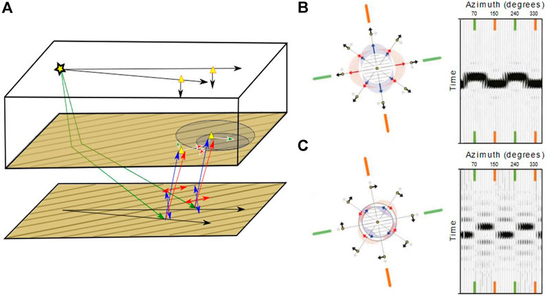
FIGURE 1. Diagram illustrating shear wave splitting (modified after Bale et al., 2009) at two ocean bottom seismometers located in, or close to a pockmark, sitting within seabed sediments containing vertical parallel fractures (HTI). (A) The pockmarks are shown as concentric circles on the seabed. Direction of shading indicates orientation of the vertical fractures. The lower surface (reflector) is the base of the anisotropic layer, across which S-wave conversion occurs. Yellow star shows location of an airgun shot near the sea surface. Yellow triangles are ocean bottom seismometers: black outline = on seafloor, red outline = projected to sea surface, to indicate the sagittal (shot – receiver) azimuth. Radial and transverse directions are indicated by black arrows. The white arrows represent the horizontal geophone orientations: green = X; red = Y component. The green arrow is the down-going P-wave phase. Fast (S1) and slow (S2) S-waves are represented with red and blue arrows respectively and their particle motions are indicated by double-ended red and blue arrows. (B) Aligned vertical fractures with 70°N azimuth viewed from the top indicating the amplitudes of fast (red arrows) and slow (blue arrows) S-waves in radial direction (black arrows) and corresponding radial seismogram. Green and orange arrows lines indicate the fracture parallel and fracture perpendicular directions. (C) same as b, transverse component. The presence of HTI is easily identifiable from the azimuthal variation seen on the radial and transverse components.

Pockmarks occur when fluid flow is focused and escapes from shallow, low-permeability, fine-grained surficial sediments (Hovland et al., 2002). The Scanner pockmark is a seafloor depression located in the northern North Sea (UK License Block 15/25), within the Witch Ground Basin. Large pockmarks, including Scanner, are continuously active in this area, with vigorous venting of methane (Böttner et al., 2019). At the Scanner pockmark complex, the seafloor and shallow sediments are also heavily disturbed by smaller pockmarks and palaeo-pockmarks (>1500 across 225 km²), with a principal NNE/SSW orientation, that are interpreted as dewatering features due to localized pressure changes (Gafeira and Long, 2015; Böttner et al., 2019).

On seismic reflection profiles, the large active pockmarks are commonly associated with bright spots at shallow depth, interpreted as gas-charged sediments, and are underlain by seismic chimneys or pipes, referred herein as chimneys. At the Scanner pockmark complex, the chimneys are imaged as sub-vertical columns of acoustic blanking reaching depths of several hundred meters. Chimneys have been interpreted as focused fluid migration pathways, hydraulically connecting deeper stratigraphic layers to the shallow sediment overburden (Berndt, 2005; Karstens and Berndt, 2015). Chimney-like features may also be generated as seismic artifacts due to scattering by near-surface features (e.g. Dean et al., 2015). Improved understanding of these shallow fluid flow systems is critical for assessing the integrity of future sub-seafloor Carbon Capture and Storage (CCS) sites.

Aims and Objectives

Here, we analyze data from a unique active-source seismic anisotropy experiment conducted using OBSs at the Scanner Pockmark Complex, an active methane venting seafloor depression. We investigate the presence of azimuthal anisotropy from beneath the Scanner pockmark, using SWS, and compare with results from a nearby reference site where there is no evidence for presence of gas such as seafloor gas emission, chimney structures or gas-bearing sediment. We conduct a multi-frequency seismic reflection analysis of the shallow sub-surface to constrain the geometry and azimuth of the observed geological features at the depth range resolved by the SWS analysis. We compare the seismic images with the results of SWS analysis to provide a complete characterization of the shallow subsurface structure directly beneath the Scanner pockmark. The SWS analysis is complemented by laboratory measurements of S-wave velocities which, in conjunction with seismic stratigraphy, enable the depth of the anisotropic layers in conjunction with seismic stratigraphy to be determined. The key aim of this study is to develop a further understanding of the structural control on fluid-escape at the Scanner Pockmark Complex by resolving the orientation and network geometry of the subsurface heterogeneities. In this paper we focus on observations of SWS from very shallow interfaces (< 10 m); future studies will investigate SWS over a greater depth range.

Stratigraphy and Seismostratigraphic Framework

The Scanner pockmark is a composite feature comprising two overlapping seabed pockmarks (East and West Scanner), with a combined size of ∼900 m × 450 m wide and depth of 22 m, lying in ∼155 m water depth. Direct evidence for methane venting is provided by the water column imaging of Li et al. (2020), who calculate a gas flux of 1.6 and 2.7 × 10⁶ kg/year (272–456 l/min), as well as the presence of methane-derived authigenic carbonate (MDAC) recovered from within the pockmarks, which formed due to anaerobic oxidation of escaping methane (Judd and Hovland, 2009).

The seismostratigraphy and lithostratigraphy hosting the Scanner pockmark complex comprises a ∼600 m-thick Quaternary sediment succession that has been described previously (Stoker et al., 2011; Böttner et al., 2019; Robinson et al., 2020), where it is sub-divided into five units, S1 to S5 (Figures 2, 3). Deposited within the Witch Ground basin, this stratigraphic complex is underlain by the Hordland and Nordland Groups, of Palaeogene and Neogene age respectively, which are composed of low-permeability claystone (Judd et al., 1994). The Scanner pockmark depression erodes down to the base of the shallowest unit, S5 (the Witch Ground Formation).

FIGURE 2

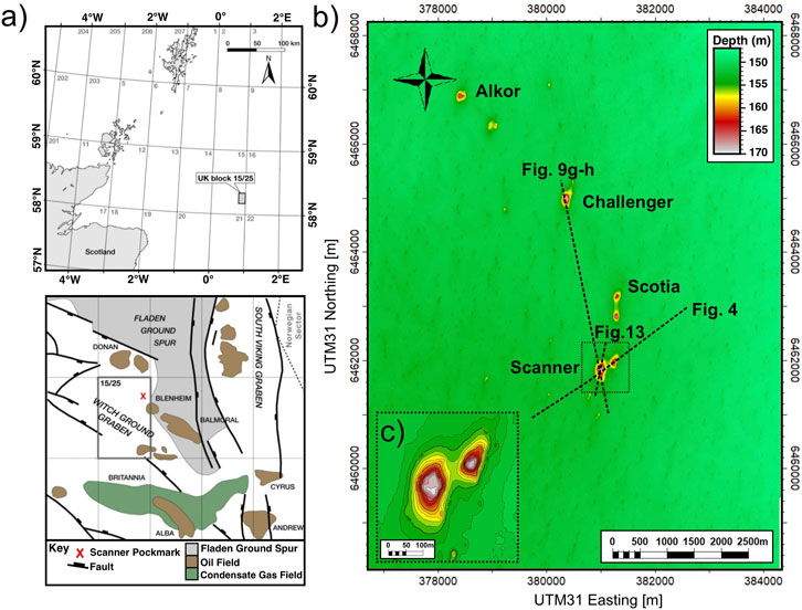
FIGURE 2. (A) Position of the Scanner Pockmark within the UK Sector of the North Sea. (B) Bathymetric map of the Scanner Pockmark Complex. Dashed lines highlight seismic lines used in Figures 4, 9G,H. Dotted square box shows inset (C). (C) Scanner pockmark, displaying East and West Scanner.

FIGURE 3

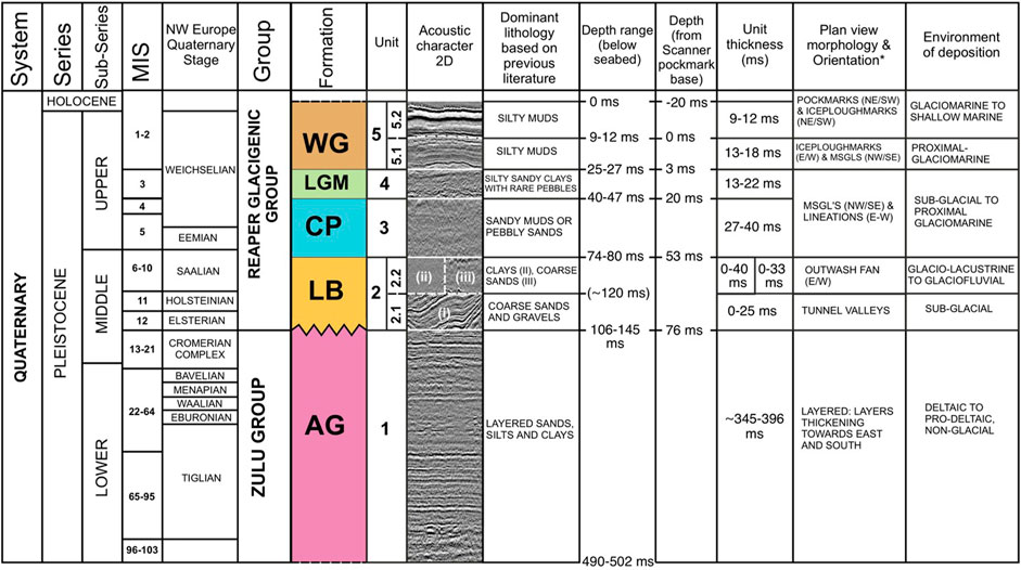
FIGURE 3. Stratigraphy of the Scanner Pockmark Complex. The chronostratigraphy, seismostratigraphy and lithostratigraphy of the Scanner Pockmark Complex is described. AG - Aberdeen Ground (purple), LB - Ling Bank (orange), CP - Coal Pit (blue), LGM - Last Glacial Maximum Deposits (green) and WG - Witch Ground (brown). The table has been created from a synthesis of Böttner et al. (2019), Ottesen et al. (2014), Stewart and Lonergan (2011), Stoker et al. (2011), Judd et al. (1994) and Andrews et al. (1990).

The Witch Ground Basin was the locus of rapid fine-grained sediment deposition between Marine Isotope Stages (MIS) 1–2, around 15–13 ka, after the end of the last glacial period (Stoker et al., 2011). Following the stabilization of sea level after the last glaciation, sedimentation into the Witch Ground Basin has become negligible, and hence the pockmarks at the current seabed demonstrate the effects of active fluid escape over at least the last 8 ka (Böttner et al., 2019).

Experiment and Datasets

In September 2017, we carried out the CHIMNEY seismic experiment around the Scanner Pockmark in the North Sea using RRS James Cook (cruise JC152) (Bull, 2018; Bull et al., 2018; Robinson et al., 2020), acquiring wide-angle and multi-channel seismic and high-frequency acoustic recordings.

Ocean Bottom Seismometer Data

A total of 25 four-component OBSs were deployed during the survey. These instruments were equipped with three orthogonal 4.5 Hz geophones fixed rigidly to the instrument frame, and a hydrophone. The OBS sampling rate was 4 kHz. Eighteen OBSs were deployed around the Scanner pockmark, with two instruments located within the pockmark (Figure 4). The OBS spacing was generally 200 m, with closer spacing within the pockmark. Seven OBSs were also deployed with 200 m spacing at a reference site, that displayed no evidence for water column venting, or subsurface fluid migration.

FIGURE 4

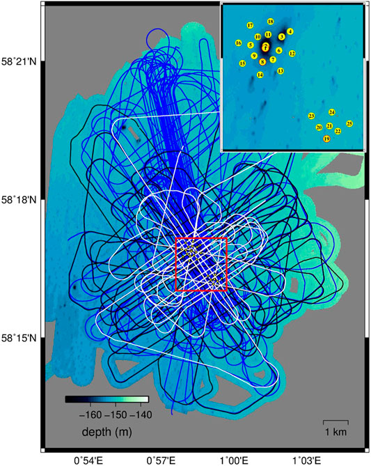
FIGURE 4. Map of the CHIMNEY seismic experiment. Black, white and blue profiles represent GI-gun, Squid 2000 sparker and sub-bottom profiler shots respectively. The 3D seismic volume extends over the entire area displayed. Yellow dots are the OBSs. Red square shows the location of the inset. Inset shows the location of the OBSs around the Scanner pockmark and at the reference site. OBSs 1, 8 and 19 shown in Figures 6–8 are surrounded in red.

All 25 OBSs recorded shot profiles acquired using five different seismic sources: Bolt and GI airguns, Squid and Duraspark surface sparkers and a deep-towed sparker. For the SWS study we used the shots acquired with the GI-gun source (2 × 210 in³), which generated frequencies of 3–300 Hz. The geometry of the GI-gun profiles (Figure 4) was chosen to be an asterisk to ensure even azimuthal coverage at all offsets and simplify the processing. Four profiles were centered on the Scanner pockmark at an azimuth interval of 45° and with lengths greater than 10 km (Figure 4). A grid of profiles of 326° and 146° azimuth was also acquired to obtain full azimuthal coverage for the SWS study and a well-sampled shot coverage for seismic tomography. The shooting interval was 8 s, equivalent to 18.5 m at the mean vessel speed of 4.5 kn.

The shot positions were calculated initially by backprojecting the ship’s GPS position to the airgun position, 84.1 m behind the ship. OBSs were deployed by free fall. Although the shallow water environment (∼150 m) reduced the difference between drop and seabed positions, the small scale of our target requires that the positions of instruments and shots are defined precisely. Therefore, we used a grid search algorithm to find the optimal average water velocity (1490 m/s), receiver locations and delay time (which accounts for airgun depth variations and for feathering), by minimizing the sum of the squared residuals between observed and predicted direct arrival times at every point of the grid. Receiver depths were not included in the inversion as the seafloor dips are small and depth differences between deployment locations and relocated positions were already within the 0.5 m uncertainty expected from the fitting algorithm.

The SEG convention for four-component seismic records (Brown et al., 2000) is used for display of the geophone and hydrophone polarities. Accordingly, the direct wave has positive polarity on the vertical geophone and negative polarity on the hydrophone. The up-going P-waves reflected from positive impedance contrasts are recorded with negative polarities on the vertical geophones. This is also the case on the hydrophones, which measure the pressure rather than a vector quantity. The x-geophone is considered to be positive when the distance vector from the shot to receiver is positive in Cartesian coordinates and the y-geophone is positive 90° clockwise from the positive x direction (Brown et al., 2000).

Seismic Reflection Data

Four different seismic sources (GI guns, Applied Acoustic Engineering Squid 2000 and Duraspark surface sparkers and a deep-towed sparker) were recorded by two different streamers (60-channel, University of Southampton, 120-channel, GeoEEL, TTS), operated at times separately and at times simultaneously (Robinson et al., 2021). In addition, a chirp source was used to acquire single-channel seismic data in sub-bottom profiler (SBP) mode. The experiment produced a broad-band seismic dataset, with frequencies from 3 to 6000 Hz.

In this study we use the SBP and Squid 2000 sparker data to generate 2D seismic reflection images around the Scanner pockmark. The SBP data were acquired using a chirp sweep lasting 0.035 s, with a bandwidth of 2.8–6 kHz, and a central frequency of 4.4 kHz. Over 100 SBP profiles were recorded (Figure 4). These profiles have a trace spacing of 2.5 m and a very high vertical resolution of <15 cm. The Squid 2000 surface sparker data were acquired at an energy of 2000 J giving a 80–1800 Hz source bandwidth and 2 s shot interval (∼4.6 m at 4.5 kn), recorded by the two streamers (Figure 4). Thirteen Squid profiles were acquired across the Scanner pockmark and processed using a time-domain workflow outlined in Provenzano et al., (2020). These profiles have a cdp-trace spacing of 2 m and a vertical tuning thickness resolution <0.45 m.

3D time-migrated seismic data were also provided by PGS (CNS MegaSurveyPlus) for the purposes of this study (Figure 5C). The 3D seismic survey used in this study covers an area >500 km² and a depth of 1.5 s two-way travel time (TWT). The full-stack data has a trace spacing of 12.5 m and a vertical resolution of approximately 5–10 m.

FIGURE 5

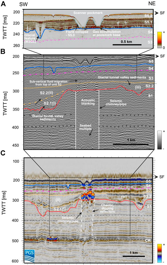
FIGURE 5. Seismostratigraphy of the Scanner Pockmark region. The seismic profiles extend from southwest to northeast across the Scanner Pockmark Complex. (A) Sub-bottom profiler seismic reflection data. (B) 2D seismic reflection data acquired using Sparker source. (C) 3D seismic reflection data. Interpreted seismic units CR and S1 to S5 are shown. CR - Crenulate Reflector (top of Nordland Group), S1 – Aberdeen Ground Fm., S2 – Ling Bank Fm., S3-4 – Coal Pit Fm [S3 – Coal Pit and S4 – Last Glacial Maximum deposits (LGM)], S5 – Witch Ground Fm (S5.1 – Fladen Member, S5.2 – Witch Member, S5.3 - Glen Member). Black dashed line = CR; red line = top S1; orange dot-dashed line = top S2.1; orange dashed line = top S2.2; pink dot-dashed line = top S3; blue line = top S4; pale brown dashed line = top S5.1 and black line = top S5.2/SF = Seafloor. Outline of a chimney is displayed with sub-vertical white dashed line. TWT values here are milliseconds below the sea surface.

Methods

Ocean Bottom Seismometer Data

P- to S- converted (C-) waves were studied using GI-gun shots on all 25 OBSs of the CHIMNEY survey network. We rotated the horizontal seismograms into radial and transverse directions, by trace by trace minimizing the power ratio of the amplitude of radial and transverse components (Haacke and Westbrook, 2006). We first flattened the direct water wave by applying a static time shift as a function of the shot-receiver offset (i.e. linear move out). Only shots up to 300 m offsets were used because at greater offsets it was difficult to distinguish the direct wave from other arrivals. The power ratios of the amplitudes were calculated on a window of 3 ms half-length centered on the direct wave arrival flattened to 0 s. The trace-by-trace minimization was done by stepwise incrementing the optimum orientation angle for x geophone using the Seismic Unix (Stockwell, 1997) compatible surttmp software of Haacke and Westbrook (2006). We searched for the optimum rotation angle between 0° and 180° to cover the whole range of possible azimuths. Instead of using a single rotation angle for all shots, with the trace-by-trace estimation of the optimum rotation angle we obtained a rotation angle for each shot. This approach accounts for possible residual uncertainties in shot and OBS locations (< 0.5 m) and the potential effects of OBS tilt.

The resulting radial and transverse components were visualized in a composite plot (Supplementary Figure S1) to check the efficiency of the rotation. A difference of two orders of magnitude is observed in the amplitude of the direct water wave observed on the radial and transverse components of all studied OBSs indicating a successful rotation. The P-wave energy is visible on the radial component but diminished on the transverse component. Radial and transverse components of the OBSs were then stacked in 9° bins of sagittal (shot-receiver) azimuth. No filtering was applied during processing because filters modify the arrival times of short offsets used in this study and C-waves are easily identified without filtering (Figures 4, 6).

FIGURE 6

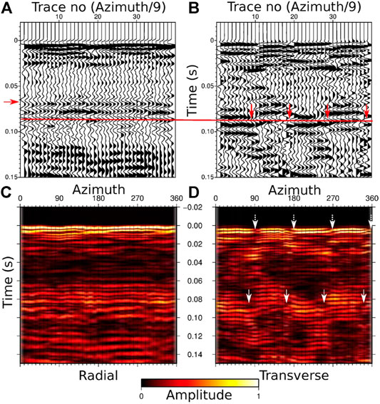
FIGURE 6. 9° azimuth stacks recorded on OBS1 located within the pockmark. Left and right panels show radial and transverse components respectively. (A) Radial wiggle plot. The red arrow shows the arrival time (∼65 ms TWT) of the C-wave phase on the radial seismogram. Red line shows the time at which the event is observed with highest amplitude due to ringing (see text). (B) Transverse wiggle plot. Red arrows show the polarity changes at 90° interval. (C) Radial envelope plot of the amplitudes (root of squared amplitudes). (D) Transverse envelope plot. White arrows show the amplitude nulls at ∼90° intervals, corresponding to the orientation of the anisotropy axes (70 and 150°). Dashed white arrows at t = 0 indicate the geophone orientations.

Seismic Reflection Data

The reflection data were interpreted using Schlumberger’s Petrel software. Over 5400 breaks in the lateral continuity of seismic reflectors were observed on a total of 104 SBP lines (Supplementary Figure S2). Such discontinuities can be created by faults, fractures, and other geological features, such as ice ploughmarks. The dense spacing of the 2D data (Figure 5) allowed the discontinuities, which crosscut the seismic profile directions, to be mapped with confidence from profile to profile. The length and net azimuth of the discontinuities (within the range of 0° - north to 180° - south) were then derived. Due to the uneven spatial distribution of the 2D profiles (Figure 4), the approach taken was to produce RMS amplitude maps over a time window of ±2.5 ms TWT around the picked horizon (top S4). This approach also had the advantage that no errors would be introduced in any depth conversion due to uncertainties in sub-surface velocities.

Macro-scale geological features and discontinuities (> 12.5 m) were also observed on time surfaces of the 3D seismic data. Where horizons were laterally continuous within the 3D data across the full study area (e.g. top of the unit S4), a surface map was produced. Where deeper horizons were laterally discontinuous, a time slice map approach was used in a similar manner to the near-surface SBP data.

Laboratory S-Wave Measurements

Knowledge of the S-wave velocities within the shallow sediments (<10 m depth) was needed to estimate the conversion depth of C-waves and thus the depth of the anisotropic layer. S wave velocities were determined from analysis of sediments cores collected during. RV Maria S Merian cruise MSM78 (Karstens et al., 2018). Sediment cores were collected from beneath the Scanner pockmark and a site 6 km northeast of the Scanner pockmark complex using a gravity corer and rock drill (RD2; British Geological Survey). A maximum penetration depth of ∼6 and ∼33 mbsf (meters below seafloor) was reached beneath the Scanner pockmark and the NE site, respectively. S-wave velocity measurements were taken in the Rock Physics laboratory of the National Oceanography center. S-wave velocity measurements were carried out on samples from four cores. The measurements were of the transmission type between two bimorph transducers inserted in to split core with their motion transverse to core major axis. Separation between transducers centers was ∼80 mm. The excitation signal consisted of a two cycle cosine wave with a center frequency of 1 kHz multiplied by a Blackman-Harris window to limit high frequency content, thus reducing and supressing the production of P-wave precursors higher in the frequency spectrum (Supplementary Figure S4). Both, the input and transmitted signal were recorded using an oscilloscope. Processing was performed in two separate ways to reduce measurement uncertainty and cross-validate results (Supplementary Figure S4). The first method was a time-of-flight approach performed in the time domain. The first major peak of the input and transmitted signals were picked. The time difference between the two picks and the distance between transducers was used calculate shear wave sound speed. The first major peak, rather than first break, was chosen because this was less affected by any residual P-wave precursor signals. The second processing method was performed in the frequency domain and is based upon the rate of change of phase with respect to frequency. The input and transmitted time domain signals were windowed using a Tuckey window to remove the P-wave precursor, multiple reflections and multi-path signals after the direct wave. The windowed signals were de-convolved in the frequency domain and a least squares linear fit to the slope of the phase with respect to frequency was calculated. The gradient of the linear fit, which is proportional to the reciprocal of sound speed, was then used to calculate sound velocity. Sources of error for these measurements include multiple reflections, propagation modes other than pure shear wave modes and p wave precursors. System time delays, the acoustic center of the transducers and measurement accuracy were estimated by making multiple measurements over distances of 0.05–0.2 m acoustic path length on a 0.5 by 0.3 by 0.3 m slab of homogeneous Potter’s clay. These reference measurements were then compared to measurements of the same Potter’s clay in split core liner over a 0.1 m acoustic path similar to that used in the experiment. From comparison to these calibration data a typically 2σ measurement accuracy of 10% is expected.

Results

Seismic Anisotropy

In this paper, two-way travel-time (TWT) values are given as milliseconds below the seafloor, unless stated otherwise. Two potential C-wave reflectors are observed at 45 and 65 ms TWT on the radial component of OBS1, located within the Scanner pockmark (Figure 6). Both reflections have apparent velocities of ∼1500 m/s, as expected for signals that have most of their raypath in the water column.

On all OBSs, the direct water wave arrival is affected by instrument ringing, most likely due to seabed coupling issues, which lasts for 25 ms. The ringing is observed on all components in different ways (Figures 6–8). A potential C-wave arrival (45 ms TWT) is visible on the radial component of OBS one as a phase clearly separated from the instrument ringing, but with a lower amplitude than the later arrival (65 ms). However, this phase is not observed on other OBSs (Figures 7, 8) as a clear arrival and is also not present on the transverse component of OBS1, suggesting that it represents either a P-wave reflection or a C-wave propagating within an isotropic medium. We interpret this early phase as a P-wave reflection from the base of seismic unit S3 (bottom of the Coal Pit Formation), since seismic units S5.1–5.2 are not present within the Scanner Pockmark, and the base of seismic unit S4 would be too shallow (20 ms TWT) to produce an arrival at this time.

FIGURE 7

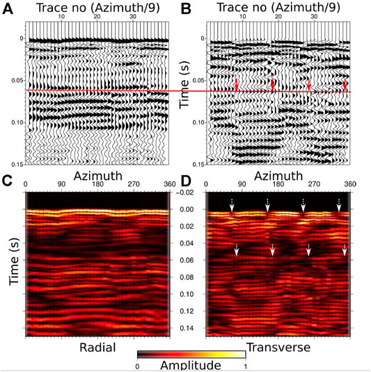
FIGURE 7. 9° azimuth stacks recorded on OBS8 located on the southwestern rim of the Scanner Pockmark. Left and right panels show radial and transverse components respectively. (A) Radial wiggle plot. The red line shows the arrival time (∼55 ms TWT) of the C-wave phase on the radial seismogram. (B) Transverse wiggle plot. Red arrows show the polarity reversals. (C) Radial envelope plot of the amplitudes (root of squared amplitudes). (D) Transverse envelope plot. White arrows show the amplitude nulls of ∼90° degree interval, corresponding to the orientation of the anisotropy axes (70 and 150°). Dashed white arrows at t = 0 indicate the geophone orientations.

FIGURE 8

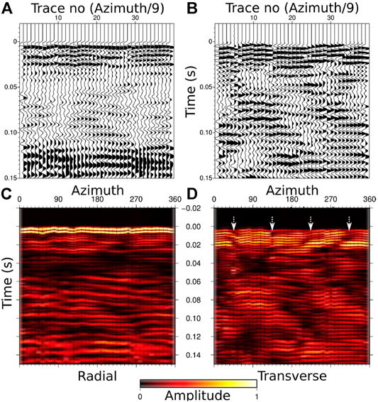
FIGURE 8. 9° azimuth stacks recorded on OBS19 located in the reference site. Left and right panels show radial and transverse components respectively. (A) Radial wiggle plot. (B) Transverse wiggle plot. No C-wave event is observed on the records of this OBS. (C) Radial envelope plot of the amplitudes (root of squared amplitudes). (D)Transverse envelope plot. Dashed white arrows (at t = 0) show the geophone orientations.

The second reflection is observed at 65 ms TWT on the stacked radial component of OBS1, and it spans on a time interval between 65 and 90 ms. The extended duration of this arrival may be due either to some instrument ringing (most likely), or the dynamic response of a localized shallow heterogeneity (Rubin et al., 2014). Polarity changes (Figure 6B) and energy nulls at ∼90° azimuthal intervals (Figures 6B–D) are observed on the transverse component, as expected for C-waves travelling within an anisotropic HTI medium. The energy nulls observed on the transverse component lie at 70° and 160° azimuths suggesting that the anisotropy symmetry axes follow these orientations. The polarity changes and the amplitude nulls are best observed at 80 ms TWT instead of 65 ms TWT, possibly because the amplitude of this event is too low to be observed at the onset of the phase, but then is amplified later due to constructive interference from the ringing. If this observed event was a residual direct water wave due to the unsuccessful rotation to radial and transverse components, the observed energy nulls would follow the geophone orientations. However, the X-geophone component of OBS1 is oriented to the north (0°), with the energy nulls at 90° intervals (Figure 6D; at 90°, 180°, 270° and 360°). There is a difference of ∼20° between the energy nulls observed on the direct wave and those observed for the C-wave event (70°–160°), and therefore we are confident of our C-wave identification. The early arrival time of the phase indicates that the S-wave conversion occurs at a very shallow reflector and the short travel time of the phase prevents the development of an observable delay between the fast and slow S-waves propagating parallel and perpendicular to the orientation of vertical fractures respectively.

A C-wave phase at 55 ms TWT (Figure 7) is observed on the radial component of OBS8. Ringing affects both the direct wave and the C-wave phase. Simultaneously, on the transverse component of OBS8, clear polarity changes are again observed, with the same azimuths as observed on OBS1 (70°–160°). Once again, there is a clear mismatch between the geophone orientations and the orientations of the anisotropy axes of the C-wave event which rules out the instrument ringing effect being misinterpreted as S-wave splitting within shallow sediments.

No potential early C-wave phase is observed on the records of the OBSs deployed at the reference site. For example, Figure 7 shows the records of OBS19. The only potential C-wave event is observed at ∼120 ms TWT with an incoherent, undulating nature on the radial component, and no polarity changes are observed on the transverse component. However, since here we focus on the SWS within the shallowest sediments, we cannot rule out the presence of deeper S-wave anisotropy around the Scanner pockmark and at our background site.

Seismic Reflection

SBP, sparker seismic reflection, and conventional 3D seismic reflection data (Figure 5) image zones with high amplitudes, characteristic of free gas within the near-surface: at 1–2 m (3 ms TWT) depth beneath the base of the Scanner pockmark complex (Figure 5A), and at 48 m (55 ms TWT) depth within the Upper Ling Bank Formation (unit S2.2; Figure 5C). Seismic chimneys are characterized on seismic images by a combination of seismic blanking and discontinuous or chaotic reflections (e.g., Løseth et al., 2011). Where free gas is present, high amplitudes are also observed at discrete intervals. The observed seismic characteristics support the interpretation that a chimney structure is present beneath Scanner pockmark (Figures 5B,C). The seismostratigraphy and observations of gas in the seismic reflection data are described in more detail by Böttner et al. (2019), Robinson et al. (2020).

Two potential causes of shallow HTI anisotropy are observed below the Scanner Pockmark (Figure 9). RMS amplitude maps derived from SBP profiles display seismic unit top S4, the uppermost sedimentary structure below the Scanner pockmark (Figures 9B,E). The presence of gas will result in a higher RMS amplitude. A prominent peak in RMS amplitude is observed at the Scanner Pockmark site, oriented at approximately 40°, and is located beneath OBS 3 (Figure 9C). The amplitude peak below OBS 3 extends towards the south west, with a small change in orientation to 50–60° azimuth below OBS1 (Figure 9C). No prominent amplitude peaks are observed at the reference site (Figures 9E,F). From a cross-sectional view, the amplitude peaks beneath the Scanner pockmark can be interpreted as due to gas-charged sediment (Figures 9G,H). The presence of gas also indicates a higher connected porosity which can be the origin of the observed S-wave splitting. In addition, the RMS amplitude maps also display areas of lower amplitude that are oriented at 50–60°, and are observed underlying several OBSs, including OBSs 1, 6, 8, 9, 14, 16, 17, and 21 (Figures 9B–E). In cross-sectional view, they are less than 80 m in width and U-shaped, with raised lateral berms, which are characteristic features of ice ploughmarks (e.g., Graham et al., 2007). Ice ploughmarks form as a result of iceberg keels coming into contact with the seafloor after calving from the marine termini of glaciers and ice sheets (Dowdeswell and Bamber, 2007). Ice-ploughmarks are common structures in the North Sea and their small dimension, and shape makes them another potential cause of S-wave splitting. In addition, sub-vertical discontinuity features can be observed on the sub-bottom profiler data within the seismic unit S5.1 (Figures 9G,H). The break in lateral continuity of the layers and minor resolvable vertical displacement may indicate the presence of fractures. These features are not visible in the sparker seismic profiles (Figure 5B) possibly because they are below the resolution of the sparker data.

FIGURE 9

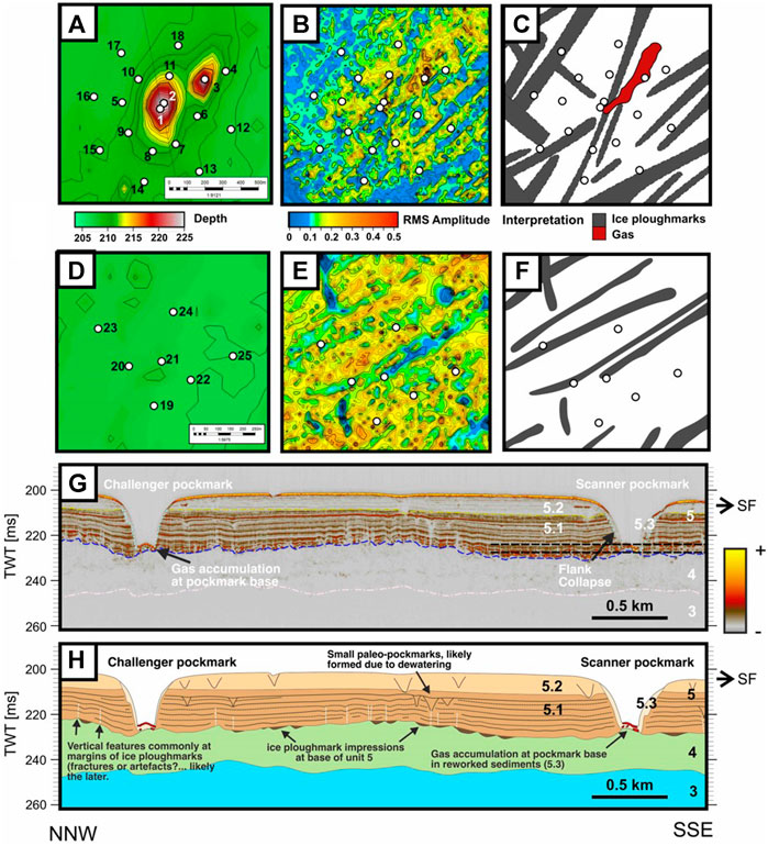
FIGURE 9. Attribute analysis and interpretation of the Scanner pockmark and reference site. Sub-bottom profiler 2D seismic reflection data is used to generate time slice attribute maps of seismic unit top S4 of (A–C) the Scanner Pockmark and (D–F) the reference site. (A, D) Bathymetry maps of seabed with OBS locations and numbers displayed. (B, E) RMS amplitude maps acquired over a time window of ±2.5 ms around the picked horizon (225–227.5 ms TWT from the sea surface); the blue areas highlight the spatial extent and orientation of ice ploughmarks. (C, F) Geological interpretation of the surface amplitude maps, highlighting gas-charged sediment (red – high amplitude) and ice ploughmarks (blue – low amplitude). (G–H) Seismic profile extending from north to south highlighting the key geological features of interest.

At a larger scale (> 12.5 m resolution) features present at the top S4 surface were also mapped using the 3D seismic data (Figure 10). We observe a clear trend of interpreted ice ploughmarks, oriented at 50–80° (Figure 10). While less evident on the length-weighted histogram (Figure 10), there is also a series of larger, more linear features oriented at 150–160° to the south west of the Scanner pockmark and reference sites. The linear features are interpreted as mega-scale glacial lineations (MSGLs), in agreement with previous interpretations of the area (e.g. Graham et al., 2007). Ice ploughmarks and MSGL trends of 50–80° and 150–160°, respectively, correlate with the azimuth of energy nulls observed on OBS1 and OBS8.

FIGURE 10

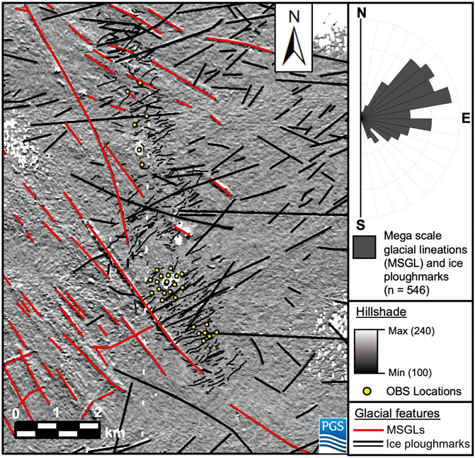
FIGURE 10. Plan view of glacial features mapped onto seismic unit top S4 (see also Supplementary Figures S2, S3). The map shows a seismic amplitude contrast (hillshade) image of unit top S4 (base of the Witch Ground Formation). Black lines display mapped ice ploughmarks and red lines display mega-scale glacial lineations (MSGLs), interpreted using the 2D and 3D seismic reflection data. A length-weighted histogram displays the most common orientation of the glacial features across the Scanner Pockmark region, binned into 10° intervals.

Between 40 and 55 ms TWT, glacial meltwater channels extend from the east across the Scanner Pockmark region (Figures 11A,B). A relatively thin channel extends into the north east of the OBS configuration with an orientation of 50–60°, underlying OBSs 1–4, (Figure 11B). The channel may be interpreted as a source for the gas-charged sediment that has been observed directly beneath Scanner Pockmark, which follows the same orientation (Figure 9C). At greater depths (60–80 ms TWT; Figure 11C), the glacial channels (corresponding to seismic unit S2.2, iii) extend further to the west, terminating at the less permeable sediments of an older glacial channel (seismic unit S2.2, ii). Gas-charged sediments are present at the stratigraphic boundary of the two sub-units (Figure 11D). Beneath Scanner pockmark, there is a clear orientation of gas-charged sediments at 50–60°, as well as an orientation of 140–150° associated with gas accumulation along the margin of the subunits (seismic units S2.2 ii and iii; Figures 10C,D). The gas accumulation appears to underlie OBSs 1–5, 9, and 11 (Figures 11C,D). The gas-charged sediment trends of 50–60° and 140–150°, also appear to correlate with the azimuth of energy nulls observed on OBS 1.

FIGURE 11

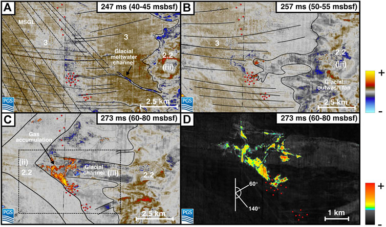
FIGURE 11. Time slice amplitude maps that provide a regional context for the presence and orientation of the shallow gas. 3D seismic reflection data is used to generate surface amplitude maps at three time intervals: (A) 40–45 ms (B) 50–55 ms and (C, D) 60–80 ms two way travel time below seafloor. Black solid lines display boundaries between seismic units or highlight key geological features. (D) RMS amplitude map, acquired over a time window of ±2.5 ms TWT, highlighting the presence and orientation of gas charged sediments; two dominant orientations of 60° and 140° are observed, which correspond to the orientation of glacial channels and the stratigraphic juxtaposition of seismic units S2.2 ii and S2.2 iii, respectively.

Core Shear-Wave Measurements

S-wave velocity measurements made of the sediment cores beneath the pockmark and at the site to the northeast are consistent and range in value between 57 and 115 m/s over a depth range of 2–22 m. There is a broad increase in velocity with depth (Figure 12) which is consistent with S-wave velocities of water-saturated clay, silty-, sandy-clay sediments (Hamilton, 1976;Hamilton, 1979).

FIGURE 12

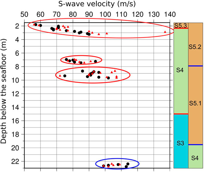
FIGURE 12. Laboratory S-wave velocity measurements. Samples surrounded by red ellipses are acquired from the pockmark and blue surrounded ones are from the reference site. Black circles are the velocities derived in time domain. Red triangles are those derived in frequency domain. Two columns represent the stratigraphy within the pockmark (left) and at the reference site (right).

Discussion

Fast S-Wave Orientation

On both OBS1 and OBS8, we observed clear SWS with consistent symmetry axes with azimuths of 70° and 160°. The delay between fast and slow S-wave arrivals observed on the radial component of the stacked azimuth versus time sections are usually used to infer the fast S-wave direction, which is commonly parallel to the fracture orientations. We do not observe significant time variations between fast and slow S-wave arrivals on the radial components of OBS1 (Figures 6, 7), likely because their travel-time as S waves is insufficient to allow the development of an observable delay and the percentage of anisotropy is low. Therefore, we cannot uniquely define the fast S-wave orientation from the analysis of the seismograms. Hence, we first analyze potential features observed on seismic profiles that may cause anisotropy and shear wave splitting. Due to the difference between the P- and S-wave velocities, especially close to the seabed where Vp/Vs is typically high (Hamilton, 1979), the up-going S-wave ray path is close to vertical (Gaiser, 2016). Therefore, any near-vertical features causing the HTI anisotropy that generates the observed SWS will be located directly below the corresponding OBSs. First, we consider the potential sources of anisotropy based on their fit to the orientation of the observed SWS. We then consider the observed arrival times of the C-wave events relative to these different potential sources of SWS, in order to attribute the observations to valid causal mechanisms.

Possible Causes of Seismic Anisotropy Within Scanner Pockmark

Regional Horizontal Stress

The regional maximum horizontal stress (σ1) is oriented NW/SE, and the average in-situ minimum horizontal stress of the region (σ3) is 54°N ± 11° (Evans and Brereton, 1990). In the region, horizontal stress exceeds the vertical stress (σ2) (Evans and Brereton, 1990). Therefore extension (tension) fractures, if present, may be expected to form perpendicular to the minimum horizontal stress (σ3), i.e. at 150–160°.

We do not observe shallow SWS on every OBSs. Only OBS 1 located within the pockmark and OBS eight located at the southwestern rim of the pockmark exhibit shallow S-wave splitting. Both OBSs are located closer to the active methane venting zone within the pockmark. The observed SWS may result from the connected porosity within the sediments that is used as migration pathways for the vertical fluid flow, aligned in the direction of the maximum regional horizontal stress. OBS 2 which is also located within the pockmark does not show any SWS suggesting that the HTI structure directly underlies the OBSs where the SWS is observed.

Local Stress

Below OBS 1, at the top S4 interface (3 ms TWT), gas-charged sediment is observed, oriented at 50–60° (Figure 9C). Gas-charged sediment is not clearly observed directly beneath OBS 8 but may be present at a scale below the horizontal resolution of the surface attribute map of 17.5 m × 17.5 m (Figures 9B,C). Where gas-charged sediment is present, gas-filled fracture corridors may form in the direction parallel to the localized overpressure gradient (e.g. Moss et al., 2003). In this case, extension (tension) fractures may form, with an orientation of 50–60°. The interpretation of gas-filled fractured sediment could explain the S-wave anisotropy directly beneath OBS 1.

Gas-charged sediment is also observed between 50–55 ms TWT with an orientation of 50–60° below OBSs 1–4 (Figure 11B), and between 60–80 ms TWT with an orientation of 140° below OBSs 1–5, 9, and 11 (Figures 11C,D). We do not observe shallow SWS on all these OBSs. However, further processing of the OBS data, including applying different normal move-out corrections to account for the increasing depth of P-S wave conversion and increase in shear-wave velocity with depth, in addition to layer stripping, to progressively correct for and remove the effects of anisotropy in shallower layers, may allow deeper SWS observations, caused by gas-filled fractures within deeper gas-bearing sediment, to be identified.

Ice Ploughmarks

Ice ploughmarks are observed at the top of unit S4. They directly underlie both OBS1 and 8 and have an azimuth of 50–70° (Figure 10). Ice ploughmarks represent an erosional surface, where icebergs have scoured the former seabed surface within a shallow glacio-marine environment. The U-shaped impressions are later filled with younger sediment, and so these could, in theory, also create anisotropy. Ice ploughmarks can act as both lateral traps and channels for fluid, creating areas of focused fluid flow (Haavik and Landrø, 2014; Chand et al., 2016). However, ice ploughmarks also directly underlie other OBSs around the pockmark and the reference site (e.g., OBSs 16, 17, 20, and 21). Therefore, despite their comparable azimuth to the observed SWS, ice ploughmarks are unlikely to be the primary cause of SWS at the Scanner Pockmark site.

Mega-Scale Glacial Lineations

MSGLs are also observed at the top S4 horizon, oriented at 150–160° (Figures 5, 10). However, the MSGL features, which represent past grounded ice in a sub-glacial environment, are not observed directly beneath the Scanner pockmark site, so we rule them out as a cause of the anisotropy observed there. It is curious that the glacial features share a similar orientation to the regional stress field of the area, posing the question of whether the two are intrinsically linked. A link may have arisen because the stress regime guides the geometry of the Witch Ground Basin and the icebergs that generated the ploughmarks were driven by contour currents along the edge of the basin.

Depth of S-Wave Conversion

Within the shallowmost water-saturated silty-clay sediments (S5, ∼18 m thick), core-logging observations indicate that the P-wave velocity is similar to the water velocity (∼1500 m/s). The corresponding S-wave velocities in shallow sediments are expected to be low and to increase with depth with a high velocity gradient (Hamilton, 1976; Hamilton, 1979). The top S4 horizon, separating units S5 and S4, is the first sedimentary boundary observed as a high-amplitude reflector on the seismic profiles. At the depth of this reflector, there are three potential features (gas-charged sediments, ice-ploughmarks and MSGLs) with similar orientations to the anisotropic symmetry axes observed on OBS1 and OBS8. Therefore, we first considered this reflector, which has an average depth of 18 m, as the interface at which the conversion occurs. With a P-wave velocity of 1500 m/s, an S-wave velocity of ∼419 m/s would be required to in order to match the arrival time of 0.055 s of the C-wave event observed on OBS 8. The Vp/Vs ratio of water-saturated silty-clay sediment varies between 13 and 7.35 in the first 20 m depth (Hamilton, 1979). In contrast, however, a Vp/Vs ratio of 3.6 is required here to match the arrival time of the C-wave event, which would be very low for these shallow sediments. We therefore ruled out the top S4 interface as the depth where the specific conversion occurs for the event observed on OBS 8.

At the NE drill site where we collected core samples and below OBS8, unit S5 exists with its full thickness. At ∼23 m depth, near the top S4 reflector, the laboratory measured S-wave velocities vary from 99 to 114 m/s (Figure 12). Considering an S-wave velocity of 100 m/s (Vp/Vs = 15), the conversion depth for the C-waves events observed on the OBS1 and OBS8 are 6.1 and 5.15 m respectively, suggesting that the conversion occurs at the top S5.1 horizon below OBS 8 (Figures 3, 9G,H). Below OBS 8, the top S5.1 horizon is observed as a bright reflector on the subbottom profiler data at 4.9 ms TWT (Figures 9, 13G,H). Below OBS1 within the Scanner Pockmark, unit S5 has a reduced thickness of 3 ms TWT (Figures 9, 13G,H) and it is reworked as it is exposed in the seafloor (unit S5.3 on Figures 9G,H). Here, unit S5.3 is underlain directly by unit S4. Within the S4 sediments, a low amplitude reflector is present on the SBP data at 7.2 ms TWT (Figure 13), which is likely to be the interface where the conversion occurs.

FIGURE 13

FIGURE 13. SBP data sampling the locations of the OBS1 and 8. The white squares are OBS 1 and 8. The low amplitude reflector is shown in black arrows. TWT values here are milliseconds below the sea surface.

Considering a P-wave velocity of 1500 m/s, the depth to the reflectors observed on the SBP data below the OBS1 and OBS8 are 5.4 and 3.7 m respectively. If the observed C-wave events are converted from the reflectors identified on the subbottom profiler data, then average S-wave velocities of 88 and 69 m/s are required to match the arrival times of 65 and 55 ms arrival times observed on OBS1 and 8 respectively. S-wave velocity measurements on samples from corresponding depths vary between 56 and 137 m/s with an average of 83 m/s. There is a good match between calculated and measured S-wave velocities, although the laboratory measurements could be affected by sampling and measurement effects (Batzle et al., 2006).

Gas-filled fractures are observed within the Coal Pit Fm (unit S3). Gravity core observations of sediment fluidization features and disseminated iron sulphide, indicates active fluid flow directly beneath the pockmark. Evidence of methane-derived authigenic carbonates and gas ebullition at this site further demonstrates that active methane venting has persisted since 27 (Böttner et al., 2019; Li et al., 2020). As shown by controlled gas release experiments in weakly consolidated sediment (e.g., Roche et al., 2020), mature gas migration from an active, focused source may take place through stable open conduits. These conduits represent channels of enhanced permeability relative to background matrix permeability (Roche et al., 2020). The very shallow conversion depth of P-S waves, together with the evidence of active gas venting within the Scanner pockmark, suggest that the SWS occurs along vertically oriented gas conduits (Figure 14). Therefore, two potential causes of anisotropy remain valid from the evidence presented: 1) aligned gas conduits, in the form of fractures, opening perpendicular to the regional minimum horizontal stress at 150–160^o, or 2) gas conduits aligned with a local stress gradient (50–60° azimuth) (Figures 5, 14)., caused by a hydraulic connection with underlying, overpressured gas charged sediment within units S2.2-S3 (Figures 5, 14).

FIGURE 14

FIGURE 14. Schematic diagram illustrating open gas migration pathways beneath Scanner pockmark that generate the shear-wave splitting observed on OBS1 and 8. Bottom right: Gas accumulations are present in S2.2, S4, and at the S4/S5.1 interface, indicated in red. Reference to color of seismic units S1-S5 found in Figure 3. Left: Blue arrows show regional maximum (σ1) and minimum (σ3) horizontal stress. Yellow arrows show local stress conditions caused by high pore fluid pressure. Red dashed line shows orientation of gas observed in Figures 11C,D. OBS locations shown in white. Top right image: S1 and S2 are the fast and slow S-wave directions, respectively.

Conclusions

We observe evidence of shear wave splitting on two ocean bottom seismometers, located within and adjacent to a pockmark which is actively venting methane. Both instruments show symmetry axes consistent with a vertically aligned fractures (HTI anisotropic system), with fracture azimuths of 70° and 160°. Based on the arrival times of the SWS events, and shallow sediment core measurements of shear-wave velocity, P- to S-wave conversions occur at 4–5 m depth beneath the seabed. Comparing these orientations and depths to potential sources for SWS, we interpret these observations as being related to vertically aligned gas conduits, which facilitate the ebullition of methane at the seafloor. These gas conduits may either result from the opening of fractures perpendicular to the regional minimum horizontal stress, or they may be aligned with the local stress gradient driven by overpressure resulting from a gas accumulation at ∼50 m depth beneath the pockmark. This study reports the first observation of very shallow anisotropy associated with active methane venting at the seabed.

Data Availability Statement

The raw data supporting the conclusions of this article will be made available by the authors, without undue reservation, to any qualified researcher.

Author Contributions

GB contributed to survey design, carried out the SWS analysis and led the manuscript writing. BC interpreted the seismic reflection data and contributed to manuscript writing. JB led the CHIMNEY survey at sea and contributed to the interpretation of the results. TM contributed to survey design, SWS analysis and the interpretation of the results. GP processed the seismic reflection data. LN carried out the S-wave velocity measurements on cores. CM calculated positions for the ocean bottom instruments and shots and contributed to the SWS analysis. AR contributed to the SWS analysis and to manuscript writing. TH led the acquisition of seismic reflection data and MC contributed to interpretation of the results from a rock physics perspective.

Funding

This work received funding from the European Union’s Horizon 2020 research and innovation programme under grant agreement No.654462 (STEMM-CCS) and the Natural Environment Research Council (CHIMNEY project: grants NE/N016130/1, NE/N016041/2 and NE/N015762/1).

Conflict of Interest

The authors declare that the research was conducted in the absence of any commercial or financial relationships that could be construed as a potential conflict of interest.

Acknowledgments

We would like to thank all those involved in the planning and acquisition of data during research cruise JC152, including the officers, engineers and crews, the scientific parties, and all seagoing technicians and engineers. The NERC Ocean-Bottom Instrumentation Facility (Minshull et al., 2005) provided the OBSs and their technical support at sea during JC152. We are also grateful for the support of Applied Acoustics Ltd. during Sparker data acquisition. We acknowledge PGS for the use of their dataset. We are grateful to Schlumberger Ltd. for the donation of Petrel software to the University of Southampton.

Supplementary Material

The Supplementary Material for this article can be found online at: https://www.frontiersin.org/articles/10.3389/feart.2021.626416/full#supplementary-material

Figure S1 | The composite plot of radial and transverse components along an inline profile recorded by 600 the OBS1. Even traces are the radial component and odd traces are the transverse component.

Figure S2 | 2D seismic vertical seismic feature picking method. Individual sub-vertical discontinuities were picked along 104 profile lines (black dots in map view – top left; and light blue in seismic cross-section view - below). Discontinuities that extended laterally across multiple 2D profiles were interpreted (black and red lines in map view – top middle and right). The discontinuities correspond to ice ploughmarks (black lines) and Mega-scale glacial lineations (red lines), respectively (Fig. 5.9).

Figure S3 | 3D seismic surface of unit top S4, uninterpreted. A seismic amplitude horizon surface (left) and hillshade map (right) is displayed.

Figure S4 | Laboratory S-wave measurements. Top: Input signal. Middle: output signal. Bottom: Frequency domain estimation of the S-wave velocity.

References

Andrews, I. J., Long, D., Richards, P. C., Thomson, A. R., Brown, S., Chesher, J. A., et al. (1990). The Geology of the Moray Firth. London: HMSO Vol. 3

Bahorich, M., and Farmer, S. (1995). 3-D Seismic Discontinuity for Faults and Stratigraphic Features: The Coherence Cube. The leading edge 14 (10), 1053–1058. doi:10.1190/1.1437077

CrossRef Full Text | Google Scholar

Bale, R., Gratacos, B., Mattocks, B., Roche, S., Poplavskii, K., and Li, X. (2009). Shear Wave Splitting Applications for Fracture Analysis and Improved Imaging: Some Onshore Examples. First Break. 27 (9). doi:10.3997/1365-2397.27.1304.32448

CrossRef Full Text | Google Scholar

Batzle, M. L., Han, D.-H., and Hofmann, R. (2006). Fluid Mobility and Frequency-dependent Seismic Velocity - Direct Measurements. Geophysics. 71 (1), N1–N9. doi:10.1190/1.2159053

CrossRef Full Text | Google Scholar

Berndt, C. (2005). Focused Fluid Flow in Passive Continental Margins. Phil. Trans. R. Soc. A. 363 (1837), 2855–2871. doi:10.1098/rsta.2005.1666

PubMed Abstract | CrossRef Full Text | Google Scholar

Böttner, C., Berndt, C., Reinardy, B. T. I., Geersen, J., Karstens, J., Bull, J. M., et al. (2019). Pockmarks in the Witch Ground Basin, Central North Sea. Geochem. Geophys. Geosyst. 20 (4), 1698–1719. doi:10.1029/2018gc008068

CrossRef Full Text | Google Scholar

Brown, R. J., Stewart, R. R., Gaiser, J. E., and Lawton, D. C. (2000). An Acquisition Polarity Standard for Multicomponent Seismic Data. CREWES Research Report. doi:10.1190/1.1815611

CrossRef Full Text

Bull, J. M., Berndt, C. B., Minshull, T. M., Henstock, T., Bayrakci, G., Gehrmann, R., et al. (2018). Constraining Leakage Pathways through the Overburden above Sub-seafloor CO₂ Storage Reservoirs. in 14th Greenhouse Gas Control Technologies Conference, Melbourne, 21-26 October 2018 (GHGT-14)

Google Scholar

Bull, J. M. (2018). Cruise Report – RRS James Cook JC152: CHIMNEY - Characterisation of Major Overburden Pathways above Sub-seafloor CO₂ Storage Reservoirs in the North Sea Scanner and Challenger Pockmark Complexes,University of Southampton, 55 pp. Available at: https://eprints.soton.ac.uk/420257/

Google Scholar

Chand, S., Thorsnes, T., Rise, L., Brunstad, H., and Stoddart, D. (2016). Pockmarks in the SW Barents Sea and Their Links with Iceberg Ploughmarks. Geol. Soc. Lond. Mem. 46 (1), 295–296. doi:10.1144/M46.23

CrossRef Full Text | Google Scholar

Crampin, S. (1985). Evaluation of Anisotropy by Shear‐wave Splitting. Geophysics. 50 (1), 142–152. doi:10.1190/1.1441824

CrossRef Full Text | Google Scholar

Dean, M., Tucker, O. D., Strijbos, F. P. L., de Jong, R. A. M., Marshall, J., and Goswami Bv, R. (2015). Characterisation and Monitoring of the Goldeneye CO2 Storage Site. Madrid: 77th EAGE Conf. Exhibition. doi:10.3997/2214-4609.201412719

CrossRef Full Text

Dowdeswell, J. A., and Bamber, J. L. (2007). Keel depths of modern Antarctic icebergs and implications for sea-floor scouring in the geological record. Mar. Geol. 243, 120–131.

Evans, C. J., and Brereton, N. R. (1990). In situ crustal Stress in the United Kingdom from Borehole Breakouts. Geol. Soc. Lond. Spec. Publications. 48 (1), 327–338. doi:10.1144/gsl.Sp.1990.048.01.27

CrossRef Full Text | Google Scholar

Exley, R. J. K., Westbrook, G. K., Haacke, R. R., and Peacock, S. (2010). Detection of Seismic Anisotropy Using Ocean Bottom Seismometers: a Case Study from the Northern Headwall of the Storegga Slide. Geophys. J. Int. 183 (1), 188–210. doi:10.1111/j.1365-246x.2010.04730.x

CrossRef Full Text | Google Scholar

Gafeira, J., and Long, D. (2015). Geological Investigation of Pockmarks in the Scanner Pockmark SCI Area. JNCC Report No 570. JNCC Peterborough. Available at: http://data.jncc.gov.uk/data/290b95b7-fcfc-4c76-8780-8714329dcf0c/JNCC-Report-570-FINAL-WEB.pdf

Google Scholar

Gaiser, J. (2016). “Chapter 7. Inversion Applications,” in 3C Seismic and VSP: Converted Waves and Vector Wavefield Applications. Editor J. Gaiser (Society of Exploration Geophysicists), 341–418. doi:10.1190/1.9781560803362.ch7

CrossRef Full Text | Google Scholar

Graham, A., Lonergan, L., and Stoker, M. (2007). Evidence for Late Pleistocene Ice Stream Activity in the Witch Ground Basin, Central North Sea, from 3D Seismic Reflection Data. Quat. Sci. Rev. 26 (5-6), 627–643. doi:10.1016/j.quascirev.2006.11.004

CrossRef Full Text | Google Scholar

Haacke, R. R., and Westbrook, G. K. (2006). A Fast, Robust Method for Detecting and Characterizing Azimuthal Anisotropy with marinePSconverted Waves, and its Application to the West Svalbard Continental Slope. Geophys. J. Int. 167 (3), 1402–1412. doi:10.1111/j.1365-246x.2006.03186.x

CrossRef Full Text | Google Scholar

Haavik, K. E., and Landrø, M. (2014). Iceberg Ploughmarks Illuminated by Shallow Gas in the Central North Sea. Quat. Sci. Rev. 103, 34–50. doi:10.1016/j.quascirev.2014.09.002

CrossRef Full Text | Google Scholar

Hamilton, E. L. (1976). Shear‐wave Velocity versus Depth in Marine Sediments: a Review. Geophysics. 41 (5), 985–996. doi:10.1190/1.1440676

CrossRef Full Text | Google Scholar

Hamilton, E. L. (1979). Vp/Vs and Poisson's Ratios in Marine Sediments and Rocks. The J. Acoust. Soc. America 66 (4), 1093–1101. doi:10.1121/1.383344

CrossRef Full Text | Google Scholar

Hovland, M., Gardner, J. V., and Judd, A. G. (2002). The Significance of Pockmarks to Understanding Fluid Flow Processes and Geohazards. Geofluids. 2 (2), 127–136. doi:10.1046/j.1468-8123.2002.00028.x

CrossRef Full Text | Google Scholar

Judd, A., and Hovland, M. (2009). Seabed Fluid Flow: The Impact on Geology, Biology and the Marine Environment. Cambridge University Press. doi:10.1017/CBO9780511535918

CrossRef Full Text

Judd, A., Long, D., and Sankey, M. (1994). Pockmark Formation and Activity, UK Block 15/25, North Sea. Bull. Geol. Soc. Denmark 41, 34–49.

Google Scholar

Karstens, J., and Berndt, C. (2015). Seismic Chimneys in the Southern Viking Graben - Implications for Palaeo Fluid Migration and Overpressure Evolution. Earth Planet. Sci. Lett. 412, 88–100. doi:10.1016/j.epsl.2014.12.017

CrossRef Full Text | Google Scholar

Karstens, J., Böttner, C., Edwards, M., Falcon-Suarez, I., Flohr, A., James, R., et al. (2018). RV MARIA S. MERIAN Fahrtbericht/Cruise Report MSM78-PERMO 2, Edinburgh, UK: Edinburgh.

CrossRef Full Text

Li, J., Roche, B., Bull, J. M., White, P. R., Leighton, T. G., Provenzano, G., et al. (2020). Broadband Acoustic Inversion for Gas Flux Quantification—Application to a Methane Plume at Scanner Pockmark, Central North Sea. J. Geophys. Res. Oceans 125 (9), e2020JC016360. doi:10.1029/2020jc016360

CrossRef Full Text | Google Scholar

Løseth, H., Wensaas, L., Arntsen, B., Hanken, N.-M., Basire, C., and Graue, K. (2011). 1000 M Long Gas Blow-Out Pipes. Mar. Pet. Geology. 28 (5), 1047–1060. doi:10.1016/j.marpetgeo.2010.10.001

CrossRef Full Text | Google Scholar

Lynn, H. B., and Thomsen, L. A. (1990). Reflection Shear‐wave Data Collected Near the Principal Axes of Azimuthal Anisotropy. Geophysics 55 (2), 147–156. doi:10.1190/1.1442821

CrossRef Full Text | Google Scholar

Minshull, T. A., Sinha, M. C., and Peirce, C. (2005). Multi-disciplinary, Sub-seabed Geophysical Imaging. Sea Technology 46 (10), 27–31. Available at: http://eprints.soton.ac.uk/id/eprint/18172.

Google Scholar

Moss, B., Barson, D., Rakhit, K., Dennis, H., Swarbrick, R., Evans, D., et al. (2003). “Formation Pore Pressures and Formation Waters,” in The Millennium Atlas: Petroleum Geology of the Central and Northern North Sea. Editor D. Evans (Geological Society of London), 317–329.

Google Scholar

Ottesen, D., Dowdeswell, J. A., and Bugge, T. (2014). Morphology, Sedimentary Infill and Depositional Environments of the Early Quaternary North Sea Basin (56°-62°N). Mar. Pet. Geology. 56, 123–146. doi:10.1016/j.marpetgeo.2014.04.007

CrossRef Full Text | Google Scholar

Provenzano, G., Henstock, T. J., Bull, J. M., and Bayrakci, G. (2020). Attenuation of Receiver Ghosts in Variable-Depth Streamer High-Resolution Seismic Reflection Data. Mar. Geophys. Res. 41, 1–15. doi:10.1007/s11001-020-09407-9

CrossRef Full Text | Google Scholar

Robinson, A. H., Callow, B., Böttner, C., Yilo, N., Provenzano, G., Falcon-Suarez, I. H., et al. (2020). Multiscale Characterisation of Chimneys/pipes: Fluid Escape Structures within Sedimentary Basins. Int. J. Greenhouse Gas Control. doi:10.5194/gmd-2019-304-rc2

CrossRef Full Text | Google Scholar

Roche, B., Bull, J. M., Marin-Moreno, H., Leighton, T., Falcon-Suarez, I. H., White, P. R., et al. (2020). Time-lapse Imaging of CO₂ Migration within Near-Surface Sediments during a Controlled Sub-seabed Release Experiment. Int. J. Greenh. Gas Control. In press.

Google Scholar

Rubin, S., Shtivelman, V., Keydar, S., and Lev, A. (2014). Seismic Ringing Effect in the Shallow Subsurface. Near Surf. Geophys. 12 (6), 687–696. doi:10.3997/1873-0604.2014030

CrossRef Full Text | Google Scholar

Stewart, M. A., and Lonergan, L. (2011). Seven Glacial Cycles in the Middle-Late Pleistocene of Northwest Europe: Geomorphic Evidence from Buried Tunnel Valleys. Geology. 39 (3), 283–286. doi:10.1130/g31631.1

CrossRef Full Text | Google Scholar

Stockwell, J. W. (1997). Free Software in Education: A Case Study of CWP/SU: Seismic Un*x. The Leading Edge 16 (7), 1045–1050. doi:10.1190/1.1437723

CrossRef Full Text | Google Scholar

Stoker, M. S., Balson, P. S., Long, D., and Tappin, D. R. (2011). An Overview of the Lithostratigraphical Framework for the Quaternary Deposits on the United Kingdom Continental Shelf. Nottingham, UK: British Geological Survey. doi:10.21236/ada557589Available at: http://nora.nerc.ac.uk/id/eprint/15939

CrossRef Full Text

Thomsen, L. (1999). Converted‐wave Reflection Seismology over Inhomogeneous, Anisotropic Media. Geophysics 64 (3), 678–690. doi:10.1190/1.1444577

CrossRef Full Text | Google Scholar

Tsvankin, I., Gaiser, J., Grechka, V., Van Der Baan, M., and Thomsen, L. (2010). Seismic Anisotropy in Exploration and Reservoir Characterization: An Overview. Geophysics. 75 (5), 75A15–75A29. doi:10.1190/1.3481775

CrossRef Full Text | Google Scholar

Wild, P. (2011). Practical Applications of Seismic Anisotropy. First Break 29 (5).

Google Scholar