Accounting for Natural Uncertainty Within Monitoring Systems for Induced Seismicity Based on Earthquake Magnitudes

1. Introduction

The increasing number of industrial operations related to hydrocarbon extraction, geothermal power production, hydraulic fracturing for shale gas exploitation, wastewater injection, water impoundment, hydrocarbon storage, and mining operations in recent years, and the potential for large-scale subsurface CO₂ storage in future, has increased the importance of understanding and de-risking induced seismicity both to the scientific community and to the public who live near such operations (Grigoli et al., 2017). The potential to induce seismicity by human activities is well-known (McGarr et al., 2002; Elsworth et al., 2016; Foulger et al., 2018; Keranen and Weingarten, 2018; Schultz et al., 2020). Military waste fluid injected in the Rocky Mountain Arsenal in the 1960's near Denver, Colorado (Healy et al., 1968), induced the so-called “Denver earthquakes.” Since then induced earthquakes related to mining (Arabasz et al., 2005; Fritschen, 2010), oil and gas field depletion (Bardainne et al., 2008; Van Thienen-Visser and Breunese, 2015) shale gas exploitation (Bao and Eaton, 2016; Clarke et al., 2019; Lei et al., 2019), geothermal exploitation (Häring et al., 2008; Deichmann and Giardini, 2009), and waste water disposal (Ellsworth, 2013) have been documented around the world (Baisch et al., 2019). In the UK, induced earthquakes related to hydraulic fracturing at Preese Hall (Clarke et al., 2014), and Preston New Road (Clarke et al., 2019) have been observed, and the latter led to an indefinitely imposed UK government moratorium on fracking.

Traffic light systems (TLS; Bommer et al., 2006; Majer et al., 2012; Mignan et al., 2017; Baisch et al., 2019) are used widely to manage hazard and risk due to induced seismicity in geothermal and hydrocarbon industries, whereby operations are continued (“green”), amended (“amber”), or stopped (“red”) based on the local event magnitude. In the original TLS developed by Bommer et al. (2006), the TLS thresholds are based on peak ground velocity, but other TLSs have been implemented based on earthquake magnitude or other ground motion parameters, such as peak ground acceleration (Ader et al., 2020). Depending on the industrial activities, criteria for a TLS may be very different. Baisch et al. (2019) and He et al. (2020) summarized some examples of existing TLSs that correspond to different industrial activities. In the UK the “amber” and “red” thresholds for induced seismicity related to unconventional oil and gas operations are set to local earthquake magnitudes M_L = 0 and M_L = 0.5, respectively, and this has led to multiple halts of hydraulic fracturing operations during the past few years (Clarke et al., 2019) and finally to an immediate moratorium of operations in November 2019.

The thresholds between zones in TLS are often defined based on limited case studies and on a priori assumptions in a best effort to provide simple schemes (Grigoli et al., 2017; Baisch et al., 2019). Consequently, they do not necessarily take into account the range of possible scenarios, nor uncertainties in event magnitudes, and hence some operations will incorrectly continue, increasing the risk of larger triggered earthquakes, while others will be wrongly halted. To ensure actions taken are robust, it is therefore necessary to estimate local magnitudes with uncertainties, and to consider them in the choice of M_L thresholds in TLSs.

Assessing accurate magnitudes for human-induced earthquakes such as shale gas stimulation, waste water storage, or enhanced geothermal systems is difficult, because they are affected by lack of knowledge about the Earth's subsurface between the source and receivers and by the magnitude scale used (Kendall et al., 2019). A standard approach to determine M_L is to first locate the earthquake and then apply an empirical scaling relation to the source-to-receiver distance (Gutenberg and Richter, 1942; Gutenberg, 2013). Source location-related uncertainties in M_L can then be evaluated using the location confidence ellipses. Unfortunately, estimating errors on M_L due to velocity model uncertainties, energy attenuation during propagation or site effects such as wavefield focusing is difficult.

It is well-known that the accuracy of hypocenter locations depends largely on the velocity model accuracy (Husen and Hardebeck, 2010). Various efforts have been made to estimate velocity model uncertainties, by including a correction term to traveltime curve predictions (Myers et al., 2007), making random perturbations around a given velocity model (Poliannikov et al., 2013) and by locating seismic events in an ensemble of velocity models obtained by a Bayesian analysis of independent data (Gesret et al., 2011; Hauser et al., 2011). Recently, Garcia-Aristizabal et al. (2020) analyzed different sources of uncertainty that can be relevant for the determination of earthquake source locations, and introduced a logic-tree-based ensemble modeling approach for framing the problem in a decision-making context. Their approach, however, is not fully probabilistic, but limited to a finite set of explored models.

Here we propose a way to calculate local magnitudes with uncertainties for microseismic events, and to include the uncertainties in the design of TLS. We use a 3D Monte Carlo non-linear traveltime tomography method to jointly invert for hypocenter locations and velocity model. This allows us to obtain posterior distributions for local magnitude M_L, which cover both velocity and source location uncertainties. Results clearly show that velocity uncertainties and station site effects are significant and change the zones of the TLS to which events are assigned, hence they directly affect safety related decisions. We then apply our method to the hydraulic fracturing induced seismicity at Preston New Road, UK and a mining site, and demonstrate that a red-light would have been encountered earlier if uncertainties would have been accounted for in the TLS thresholds.

2. Methods and Data

Usually, local magnitudes M_L are calculated by first locating the earthquake using standard linearized earthquake location methods (e.g., Klein, 2002), which require simple assumptions about the unknown underlying subsurface seismic velocity structure, and then applying an empirical scaling relation to the source-receiver distance to determine M_L (Gutenberg and Richter, 1942; Gutenberg, 2013). The solution found by such location methods depends on the a priori best guess velocity model, and so it is not guaranteed to find a location near that of the true earthquake. They also cannot represent uncertainties on M_L related to velocity model uncertainties, energy attenuation during propagation, or site effects such as wavefield focusing.

2.1. Non-linear Joint Hypocenter-Velocity Travel-Time Tomography

We use a probabilistic approach to jointly invert for hypocenter locations and 3D subsurface velocity. Our approach is based on a reversible jump Markov chain Monte Carlo algorithm (Green, 1995), which is an iterative stochastic method to generate samples from a target probability density. In a Bayesian approach all information is described in probabilistic terms. The goal is to calculate the posterior probability distribution function (pdf) which describes the probability of model m being true given observed data d and other relevant, a priori information. The posterior pdf is defined using Bayes' theorem (Jaynes, 2003): this combines prior knowledge about the model the prior probability p(m) with a likelihood function p(d∣m) that describes the probability of observing the data if the particular given model m was true. In our approach, the posterior probability is a trans-dimensional function: the number of parameters is not fixed, and hence the posterior pdf is defined across a number of spaces with different dimensionalities.

We use the approach and code of Zhang et al. (2020) and use arrival times of P and S body waves from local earthquakes as data, and include the velocity model, the average arrival time uncertainties, source locations and original time as parameters. The 3D subsurface velocity model is defined in terms of a Voronoi tessellation of constant velocity cells, where both the position of Voronoi cells and their number can change during sampling, guided by the data and prior information. However, due to the parsimony of Bayesian inference, complicated models (models with many cells) tend to be rejected in favor of simpler models, if they fit the data equally well. The full model vector m is given by

$\begin{array}{ll}\text{m}=(\sigma ,n,\text{s},{\text{V}}_s,{\text{V}}_p,\text{e}),& (1)\end{array}$

where n is the number of Voronoi cells, s describes their positions, and V_s and V_p describe the S- and P wave velocity within each Voronoi cell. The vector $\text{e}=\left(e_x^1,e_y^1,e_z^1,e_t^1,...e_x^N,e_y^N,e_z^N,e_t^N\right)$ contains source locations and origin times of N events, and σ is the arrival time data uncertainty. The travel time uncertainties for event i are defined as Zhang et al. (2018):

$\begin{array}{ll}{\sigma }_i={\sigma }_0{t}_i+{\sigma }_1,& (2)\end{array}$

where σ₀ and σ₁ are noise hyperparameters and t the P or S travel time.

We initialize 20 Markov chains with randomly generated starting models drawn from the prior distribution so that each chain starts from a different point in model space. To minimize dependence on this initial model, chains progress through a large number of samples called the burn-in phase from which all models are discarded. To reduce dependence of each sample on the next, after burn-in we only store every 200th model to use as samples of the posterior distribution. Each chain sampled 1.88 million models. At each step of the Markov chain a new model m′ is generated by perturbing the current model. In our approach we have seven types of possible perturbation: adding, removing or moving a Voronoi cell (i.e., changing s), changing the P or S velocity of a randomly chosen Voronoi cell (V_p, V_s), changing the noise hyperparameter σ, or changing the source coordinates of one randomly chosen source (e). The type of perturbation is selected randomly at each iteration, and the candidate model m′ is accepted with a probability α (Green, 1995) given by:

$\begin{array}{ll}\alpha ({\text{m}}^{\prime }|\text{m})=\text{min}\left[1,\frac{\text{p}({\text{m}}^{\prime })}{\text{p}(\text{m})}\frac{\text{q}(\text{m}|{\text{m}}^{\prime })}{\text{q}({\text{m}}^{\prime }|\text{m})}\frac{\text{p}({\text{d}}_{obs}|{\text{m}}^{\prime })}{\text{p}({\text{d}}_{obs}|\text{m})}|\text{J}|\right]& (3)\end{array}$

where J is the Jacobian matrix of the transformation from m to m′ and is used to account for the volume changes of parameter space during jumps between dimensions, and q(m|m′) are proposal distributions that we use to propose new models m′ at each step. In our case, it can be shown that the Jacobian is an identity matrix (Zhang et al., 2018).

A key function in the acceptance probability is the likelihood p(d∣m) which quantifies the misfit between the observed data d_obs and estimated data d_est obtained by an eikonal solver using the fast marching method (Rawlinson and Sambridge, 2004) in model m. The likelihood is defined as:

$\begin{array}{ll}\text{p}(\text{d}|\text{m})\propto exp\left(\frac{-\varphi (\text{m})}{2}\right)& (4)\end{array}$

where

$\begin{array}{ll}\varphi (\text{m})={\displaystyle \sum _i}\frac{{\left(d_{obs}^i-d_{est}^i\right)}^2}{{\sigma }_i}& (5)\end{array}$

and σ_i is the P or S wave travel time uncertainty for event i given by Equation (2). The likelihood function contains both the effect of the errors in the source locations and the velocity model uncertainties on the travel times. We choose uniform priors for the source location coordinates and the number of Voronoi cells, and Gaussian priors for all other parameters. A full and more detailed description of the methodology can be found in Zhang et al. (2018, 2020).

2.2. M_L Scaling Relations

A general local magnitude scaling relation is described by

$\begin{array}{ll}{M}_L={log}_{10}(A)+a{log}_{10}(r)+br+c+dexp(fr),& (6)\end{array}$

where r is the hypocentral distance in km, and A is the zero-to-peak amplitude in nm on the horizontal components filtered with a Wood-Anderson response (Ottemöller and Sargeant, 2013; Butcher et al., 2017; Luckett et al., 2018). Parameters a, b, c, d, and f are region dependent constants which describe the geometrical spreading (a), attenuation (b), the base level (c), and distance dependent correction terms (d and f), respectively.

The original BGS scaling relation given by Ottemöller and Sargeant (2013) is

$\begin{array}{ll}{M}_L^{OS}={log}_{10}(A)+1.11{log}_{10}(r)+0.00189r-2.09.& (7)\end{array}$

This was updated by Butcher et al. (2017) to account for short source-receiver distances, giving

$\begin{array}{ll}{M}_L^B={log}_{10}(A)+1.17{log}_{10}(r)+0.0514r-3.& (8)\end{array}$

The M_L scaling relation now used by the BGS (Luckett et al., 2018) is:

$\begin{array}{ll}{M}_L^L={log}_{10}(A)+1.11{log}_{10}(r)+0.00189r-1.16exp(-0.2r)-2.09.& (9)\end{array}$

The latter scale was used for the BGS locations throughout this paper.

2.3. Data

We use data from surface seismic monitoring arrays at two sites in the United Kingdom: (1) Preston New Road, where hydraulic fracturing took place in the Bowland Shale tight gas reservoir, and (2) Thoresby Colliery, a deep coal mine in Nottinghamshire.

At Preston New Road, hydraulic fracturing started on 15 October 2018 at the PNR-1z well in Lancashire, UK under the guidance of Cuadrilla Resources Ltd. and targeted the Bowland shale at a depth of ~2,300 m (Clarke et al., 2019). During operations, the British Geological Survey (BGS) detected 172 local seismic events with local magnitudes M_L between −1.8 and 1.6. The M_L = 0 threshold (“amber”) was exceeded by nine events, six of which had local magnitudes larger than 0.5 (“red” zone). In late October 2018, five events occurred that exceeded the red light TLS thresholds after which operations were paused for a month, but microseismicity still occurred during the hiatus (Figure 1). The largest event with M_L = 1.6, which was felt by some local residents, occurred on 11 December 11:21:15 UTC after operations resumed on 8 December. Hydraulic fracturing operations of the well ended on 17 December 2018. Over the course of 3 months more than 38,000 microseismic events were detected in real-time with the geophone array, with moment magnitudes M_w between −3.1 and 1.6 (Clarke et al., 2019). We analyzed the P- and S-wave travel time data for the 172 largest earthquakes which were recorded at 11 seismic stations by the BGS (Figure 2). The majority of these events occurred between 2 and 2.5 km depth and occur in the vicinity of the well.

FIGURE 1

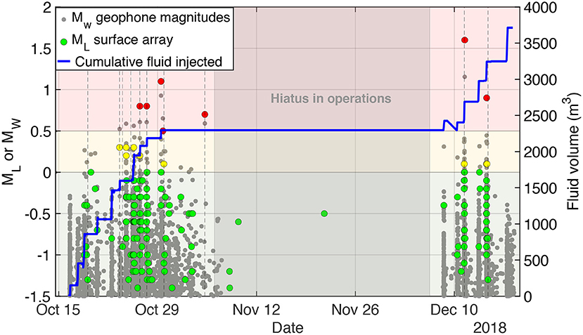
Figure 1. Induced seismicity at hydraulic fracturing site at Preston New Road, UK. Background colors indicate the three zones of the UK TLS. Smaller gray dots show the moment magnitude (M_w) for events observed on the dowhole geophone array. Larger dots show the local magnitude (M_L) for events observed by the surface seismometer array, and are color-coded by the TLS zone into which they fall. The blue line shows the cumulative volume of fluid injected into the well.

FIGURE 2

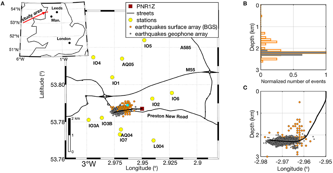
Figure 2. Seismicity at Preston New Road. (A) Seismic stations (yellow dots) near the Preston New Road hydraulic fracturing site near Blackpool (location shown in inset) and seismic events used in this study (orange dots). The injection well is shown by a black line. The cyan dot marks an earthquake discussed in Figure 5. (B) Histogram of depth distribution of the seismic events recorded at the surface array (orange) and the downhole geophone array (gray). (C) Distribution of seismic events.

2.3.1. Thoresby Colliery

Thoresby Colliery in New Ollerton has a history of seismicity related to mining (Bishop et al., 1993), and in response to felt earthquakes between December 2013 and January 2014, the British Geological Survey (BGS) installed a temporary seismic network with seven seismometer stations, four of which are three-component broadband stations (Figure 3). Mining-induced earthquakes are some of the most widely studied and their magnitude and depth range is similar to fracking induced earthquake magnitudes (Davies et al., 2013), hence provide an excellent analog for the study of hydrofracturing induced seismicity.

FIGURE 3

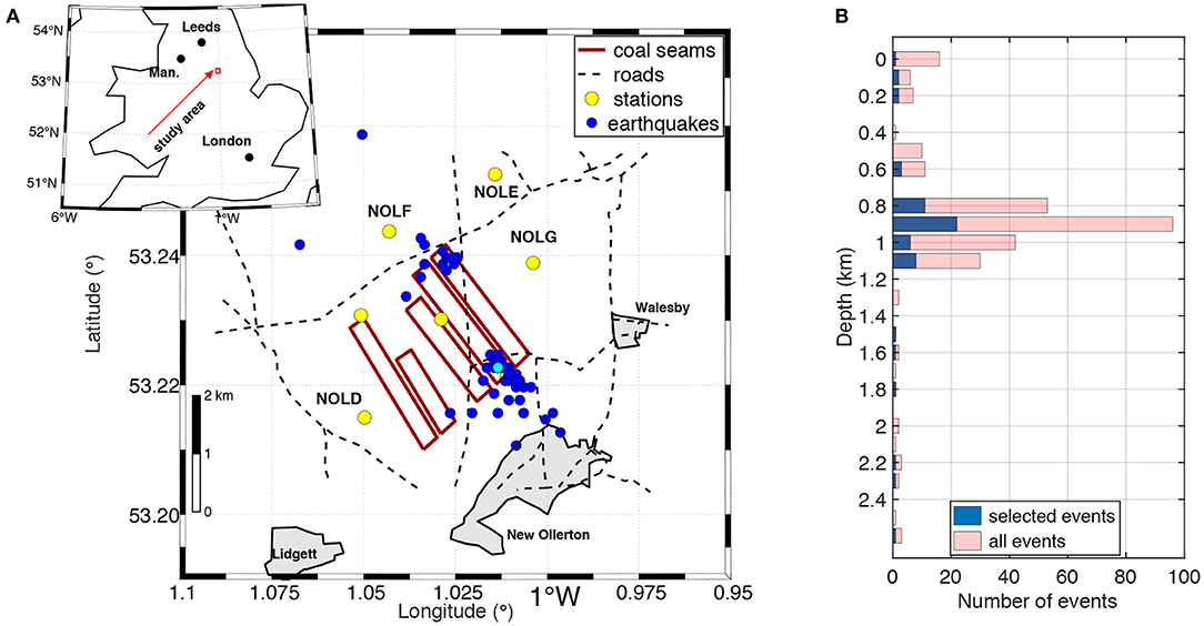
Figure 3. Seismicity at the Thoresby Colliery mining site. (A) Seismic stations (yellow dots) near the UK's last deep coal mine in New Ollerton (location shown in inset) and seismic events used in this study (blue dots). The coal seam mine galleries are outlined by red rectangles. (B) Depth distribution of the seismic events as determined by the British Geological Survey. Depths for all events in the catalog are shown in pink; the blue bars correspond to the subset of the catalog used in this study.

Most of the seismic events used in this study are located north and south of the coal seams (Figure 3), and the majority of the events occurs at 800 m depth, which coincides with the depth of the coal seams (Butcher et al., 2017). The northern cluster occurred later in 2014 than the southern one. To reduce the computational costs we only use 61 seismic events out of the 305 recorded, giving 769 P- and S travel times to invert.

3. Results

The McMC joint inversion provides us 3D posterior distributions of seismic velocities (V_p and V_s), and of the earthquake hypocenter locations (Figures 4A,B). Therefore, we can calculate hypocentral distance posterior distributions (Figure 4C), which in turn allows us to estimate station-average local magnitudes M_L posterior distributions (Figure 4D) using a scaling relation (e.g., one of Equations 6–8). These distributions include the effects of velocity and source location uncertainties as well as the source radiation pattern on the pdf for event magnitudes. The station-averaged M_L posterior distribution for one source may have a width that spans more than one zone of the traffic light system (e.g., cyan distribution in Figure 4D) which indicates that velocity model uncertainties alone can change the TLS zone to which the earthquake is attributed. Thus, uncertainties affect real operational decisions.

FIGURE 4

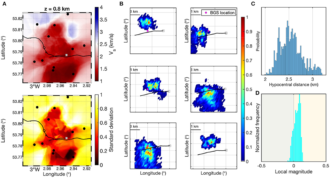
Figure 4. Results of the McMC joint hypocenter-velocity tomography at Preston New Road. (A) Shear wave velocity V_s at 0.8 km depth and its standard deviation. (B) Posterior probability distribution of hypocenter locations in longitude-latitude for six different sources. (C) Posterior probability distribution of hypocentral distance of one source to one station. (D) Posterior probability distribution of local magnitude of the same event as in (C), calculated from the hypocentral distance using the scaling relation in Equation (8).

3.1. Scaling Relation and Station Site Effects on M_L

Figure 5 summarizes uncertainties in M_L due to scaling relation and station site effects at one station at Preston New Road. We observe that the particular choice of M_L scaling relation affects the local magnitude and is itself large enough to change the TLS zone. Local magnitudes are more than half a magnitude unit larger using the original BGS scaling relation ($M_L^{OS}$, Equation 6) compared to the most recent scale ($M_L^L$, Equation 8) (Figure 5A; Supplementary Figure 1) and therefore make a difference between a continuation (“green”) and an immediate stop (“red”). Note, however, that the original BGS scaling relation was not used by the BGS to calculate M_L for these events; we include it here to show the effect of magnitude scale choices. The difference in M_L between the $M_L^B$ scale (Equation 7) and the most recent UK scaling relation $M_L^L$ (Equation, 8) are smaller, but peaks of distributions can lie in different zones of the TLS (Figure 5A).

FIGURE 5

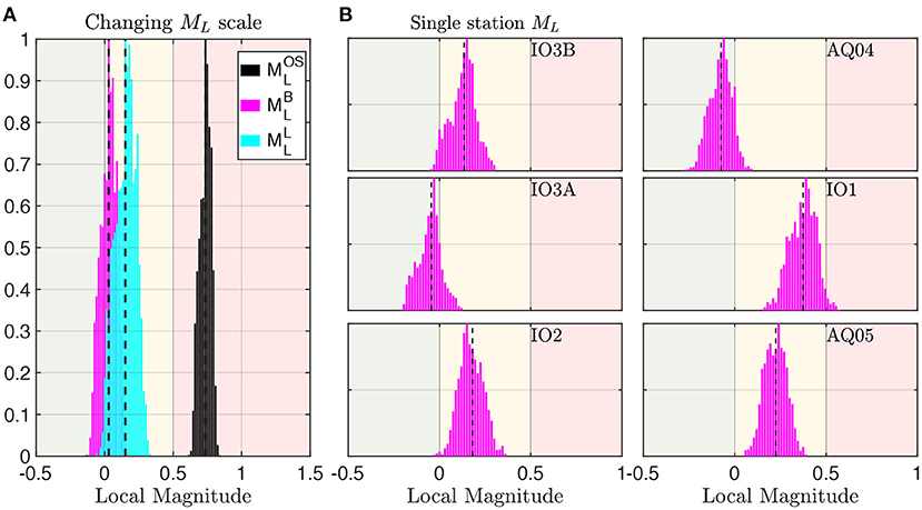
Figure 5. Effect of scaling relation and station site effects on M_L for Preston New Road stations. Local earthquake magnitude M_L posterior probability distributions for the cyan colored earthquake in Figure 1. (A) Effect of the local magnitude scaling relation (Ottemöller and Sargeant, 2013; Butcher et al., 2017; Luckett et al., 2018) (Equations 6–8). (B) Single-station magnitudes at 6 stations using Equation (7). Background colors indicate the zones of the UK traffic light system (Department of Energy and Climate Change, 2013). Dashed lines indicate the mean.

Station site effects such as attenuation, focusing, and radiation pattern become evident by comparing M_L distributions at individual stations. These uncertainties can shift the M_L posterior distribution for one source by half a magnitude unit, sometimes more, easily sufficient to move the source into another zone of the TLS (Figure 5B; Supplementary Figure 2). We compare velocity and station site effect uncertainties on local magnitudes in Figure 6 for the hydraulic fracturing induced earthquakes at Preston New Road. The site effect uncertainties are estimated by calculating the mean local magnitude for each seismic source at all 4 stations (using the amended BGS scaling relation, Equation, 8), and then taking the difference between the smallest and largest mean station magnitude as a measure of site-related uncertainties. The velocity-related uncertainties are defined as the width of the interval between the 5–95% percentile of the station-averaged local magnitudes distributions. Their effects each average around ±0.125 and ±0.05 magnitude units, respectively, in our case study, but they vary and can have a combined effect that alters magnitude estimates by up to a whole magnitude unit (Figure 6). We observe that uncertainties are also roughly equally important for the mining induced seismicity at New Ollerton—their effects average around ±0.3 and ±0.05 magnitude units for site and velocity-related effects, respectively—with a combined effect that again can alter magnitude estimates by up to a whole magnitude unit, and potentially move events from “green” to “red” zones (Figure 7).

FIGURE 6

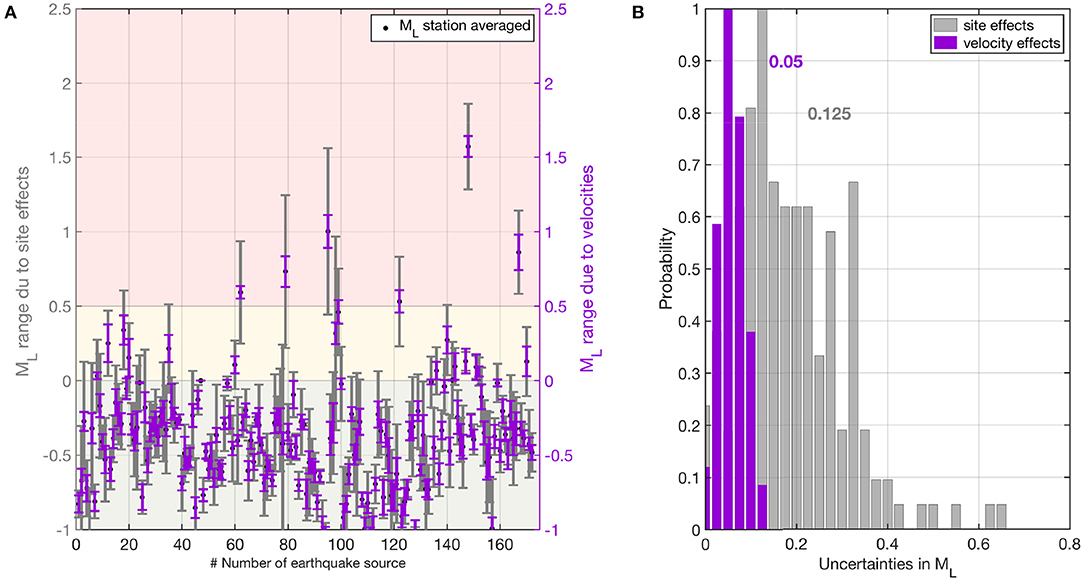
Figure 6. Comparison of velocity and station site effect uncertainties on local magnitudes at Preston New Road. (A) Uncertainties on the station-averaged magnitude calculated with the amended BGS scale (Equation 8) due to velocity uncertainties (purple error bars) and station site effects (gray bars). Black dots mark the maximum of the station-averaged M_L distribution for each seismic event. Background colors indicate the three zones of the UK traffic light system, “green,” “amber,” and “red.” (B) Normalized histograms of the magnitude uncertainties displayed in (A). Numbers display the velocity and station-site effect uncertainties at which the histograms take maximum values.

FIGURE 7

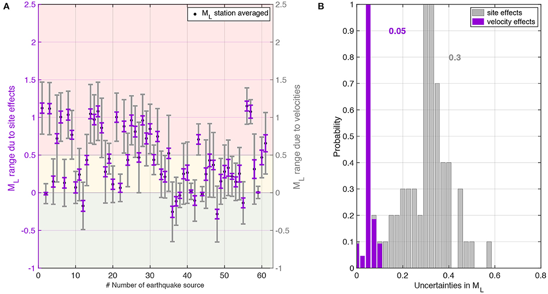
Figure 7. Comparison of velocity and station site effect uncertainties on local magnitudes at New Ollerton mining site. (A) Uncertainties on the station-averaged magnitude calculated with the amended BGS scale (Equation 8) due to velocity uncertainties (purple error bars) and station site effects (gray bars). Black dots mark the maximum of the station-averaged ML distribution for each seismic event. Background colors indicate the three zones of the UK traffic light system, “green,” “amber,” and “red.” (B) Normalized histograms of the magnitude uncertainties displayed in (A). Numbers display the velocity and station-site effect uncertainties at which the histograms take maximum values.

4. A Probabilistic Traffic Light System

We can now include the velocity and station site effect uncertainties in M_L in a traffic light system (TLS). To do this, we first calculate M_L threshold probability curves using the station-averaged M_L posterior distributions of the microseismic events at Preston New Road. Threshold probability curves describe the probability that an earthquake of a given magnitude is in any one zone of the TLS. They take into account velocity and station-site effect uncertainties, as well as attenuation and geometrical spreading in M_L. Furthermore, the threshold probability curves allow us to draw conclusions about the range of observed M_L for which the probability of any earthquake being in a zone drops below a given confidence level α. The last point is particularly interesting for regulators and operators because it enables them to define the thresholds between zones in such a way that the probability of an earthquake being in each zone of the TLS is always above a chosen confidence level α.

M_L threshold probability curves are obtained by shifting each of the 172 station-averaged event M_L pdfs along the local magnitude axis and estimating the percentage of the distribution lying in each of the three zones of the TLS (Supplementary Figure 3). By averaging over all threshold probabilities curves, we obtain one curve that describes the probability of an earthquake with a given magnitude being in any zone of the TLS. This can then be used to draw conclusions about (1) probabilities of earthquakes of a certain event magnitude M_L being in any one of the TLS zones, and (2) the M_L range for which the probability of any earthquake being in a zone drops below a given confidence level α.

Our approach here is approximate, but once the first inversion if performed, subsequent assignment of a new event's M_L to the correct zone of an adjusted TLS is trivial and can be done in real time, as explained below. In theory, however, the most rigorous approach to incorporating uncertainty into the calculation of M_L for any one event is to retrieve its full posterior M_L distribution, which is the averaged pdf across all stations for that one event. Although at this point we can do this for any existing event in our dataset, in practice we want to be able to do this for each new event that occurs, in real time. This presents a large challenge, however, since formally we must add the travel times from this new event to our dataset and re-run the whole sampling procedure again. We have added one new earthquake to the dataset and sampled 140,000 new models. This took 14,880 CPU-hours on the ARCHER HPC machine, and so remains practically impossible for real time monitoring. Furthermore, the M_L pdf of the new event is still sparsely sampled, and hence does not allow for a robust M_L uncertainty quantification.

4.1. TLS With Realistic Uncertainties

A regulator or operator can choose whether they wish to minimize the probability of any such event exceeding a TLS threshold undetected, or to maximize the certainty that an event truly has exceeded the legal magnitude limits in order to avoid unnecessary, costly halt of operations. We term the first TLS^–, where the M_L thresholds are shifted toward smaller apparent-magnitude thresholds. In this way, the risk of smaller-magnitude events leading to large earthquakes is reduced because operations are both halted and put “on caution” earlier. In the latter, the TLS thresholds would effectively be increased to higher values (TLS⁺), so that operations could still continue up to larger apparent earthquake magnitudes. The choice of the risk system by the operator (TLS⁺ or TLS^–) is, however, subjective and depends on the country's governmental policies. The choice of the confidence level defines the TLS thresholds, but these as well as the risk strategy can be changed at any time.

For example, say a regulator or operator chooses that the confidence level with which each event is assigned to the correct zone must be at least 80% for decisions to be made. The range of estimated M_L values that would have less than α = 0.8 probability is −0.036 < M_L < 0.035 (zone A) and 0.46 < M_L < 0.53 (zone B) (gray zones in Figure 8A) using the current UK TLS thresholds. Then, in a TLS^–, all of zone A would be attributed to “amber,” and zone B to “red,” effectively moving the TLS thresholds to lower values (Figure 8B). Alternatively, in a TLS⁺, zone A would be assigned to “green” and zone B to “amber,” so the TLS thresholds would effectively be increased to higher values (Figure 8C).

FIGURE 8

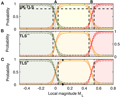
Figure 8. Developing TLS systems where the risk of larger triggered earthquakes is potentially reduced (TLS^–), and a TLS where the risk of unnecessary, costly stop of operations is reduced (TLS⁺). The threshold probability curves describe the probability of an event of local magnitude M_L being in any one of the TLS zones (color coded red/amber/green for each zone). (A) Earthquakes that have M_L estimates in zones A and B cannot be assigned to “red/amber/green” with 80% confidence. (B) For a 20% risk of an event exceeding a TLS threshold undetected, zones A and B are attributed to “amber” and “red,” respectively (TLS^–). (C) For 80% certainty that any event has exceeded a threshold, zones A and B are attributed to “green” and “amber,” respectively (TLS⁺). Black dots in (C) mark probabilities for example earthquakes of different M_L.

The uncertainties in M_L discussed here are site specific so need to be determined for each geographical area or industrial operation individually. However, our approach can be applied to any site and to any form of induced seismicity. We have also demonstrated that for the Thoresby Colliery mining site in the UK the velocity model and station site effect uncertainties in M_L are non-negligible (Figure 7), and can be accounted for in the choice of TLS thresholds (Supplementary Figure 4).

5. Application of a Probabilistic TLS to Preston New Road seismicity

We can use the three TLSs (Figure 8) to analyze retrospectively how decisions would have changed at Preston New Road under a TLS⁺ or TLS^– (Figure 9). We compare here the classification in the UK-TLS, a TLS^– and TLS⁺ for a 80% confidence level (Figure 5). That means, the risk of exceeding a TLS threshold in TLS^– is 20%, while in the TLS⁺, the certainty that a threshold was exceeded is 80%. The earthquake on October 19th would have been classified as “amber” in all three TLSs using the maximum probability magnitude, whereas it was classified as “green” by the operator. Hence, action would have been taken earlier and the probability of subsequent larger events would have been reduced. The same is true for the seismicity on October 24th (Figure 9B), where operations would have stopped immediately with a safety prioritizing system (TLS^–), and also in the UK TLS with a M_L that accounts for uncertainties. This demonstrates the importance of accounting for uncertainties in local magnitudes M_L in the decision-making process.

FIGURE 9

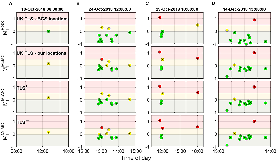
Figure 9. Classification of seismic events for 4 days (A-D) in the UK TLS (top two rows). Row 1 shows results using the local magnitudes determined by the BGS while other rows use the maximum probability magnitude determined in this work. Row 3: Classifications for a TLS where the risk of unnecessary, costly stop of operations is reduced (TLS⁺). Row 4: TLS where the risk of larger triggered earthquakes is potentially reduced (TLS^–). Both were calculated for an 80% confidence level.

We acknowledge that the occurrence of induced seismicity is a multi-parameter phenomenon, depending on details of subsurface structures as well as on the complete history of operational measures and therefore cannot be predicted. Deformation processes may continue and can still induce seismicity after injections stop. The delay time between hydraulic fracturing completion and the cessation of the observed seismicity can be up to several years (Baisch et al., 2019). It is therefore speculative that an earlier stop would have prevented large magnitude post-injection seismicity at PNR. Nevertheless, it has been shown that lower M_L threshold values in the TLS used for the geothermal stimulation in Basel, Switzerland could have prevented larger magnitude post-injection seismicity (Baisch et al., 2019). We therefore argue that it is critical to establish systems which permit regulators to account for uncertainties while managing risk, as we propose here.

6. Conclusions

We implemented a fully Bayesian approach for analysing uncertainties, such as velocity model and source location uncertainties in local earthquake magnitudes and evaluate their influence on decision-making for induced seismicity. We conclude that these uncertainties are important, as they can make a difference of up to one or two magnitude unit, and hence directly affect operational decisions by potentially moving an earthquake two zones in a traffic light system (TLS) leading to radically different operational outcomes.

To build a site-specific probabilistic TLS that accounts for uncertainties, the following three steps are necessary: (1) run one fully non-linear hypocenter-velocity tomography for the site and calculate M_L posterior distributions for each earthquake. (2) calculate threshold probability curves, choose a desired confidence level α, and determine the M_L zones A and B below the desired confidence level. (3) attribute zone A and B to “green/amber” or “amber/red” according to the desired safety system (reduce the risk of larger magnitude events (TLS^–) or reduce the risk of halting operations unnecessarily (TLS⁺)). From this point on, real time assignment of any new event's M_L to the correct TLS zone is trival, yet incorporates all the uncertainty in the measurements.

We applied our method to anthropogenic seismicity at a hydraulic fracturing site in the UK, and demonstrate that a red-light threshold would have been encountered earlier in a TLS^–, which possibly could have prevented the UK-wide shut-down. We also applied our methods to mining-related seismicity at Thoresby Colliery, UK and find they apply equally well in this different setting. Hence, our approach can be applied to any site and any form of seismicity.

Data Availability Statement

The original contributions presented in the study are included in the article/Supplementary Materials, further inquiries can be directed to the corresponding author/s.

Author Contributions

CR processed the data, performed the analysis, prepared the figures, and wrote the paper. XZ developed the inversion code. BB provided the data of both case studies. All authors contributed to the interpretation of the results and the writing of the paper.

Funding

This work was supported by the Natural Environment Research Council [grant number NE/R001154/1].

Conflict of Interest

The authors declare that the research was conducted in the absence of any commercial or financial relationships that could be construed as a potential conflict of interest.

The handling editor declared a shared affiliation with one of the authors AC at time of review.

Acknowledgments

This work used the ARCHER UK National Supercomputing Service (http://www.archer.ac.uk) and ARC3, part of the High Performance Computing facilities at the University of Leeds, UK. The authors thank the Edinburgh Interferometry Project sponsors for supporting this research. We thank two reviewers for their comments to improve this manuscript.

Supplementary Material

The Supplementary Material for this article can be found online at: https://www.frontiersin.org/articles/10.3389/feart.2021.634688/full#supplementary-material

References

Ader, T., Chendorain, M., Free, M., Saarno, T., Heikkinen, P., Malin, P. E., et al. (2020). Design and implementation of a traffic light system for deep geothermal well stimulation in Finland. J. Seismol. 24, 991–1014. doi: 10.1007/s10950-019-09853-y

CrossRef Full Text | Google Scholar

Arabasz, W. J., Nava, S. J., McCarter, M. K., Pankow, K. L., Pechmann, J. C., Ake, J., et al. (2005). Coal-mining seismicity and ground-shaking hazard: a case study in the Trail Mountain Area, Emery County, Utah. Bull. Seismol. Soc. Am. 95, 18–30. doi: 10.1785/0120040045

CrossRef Full Text | Google Scholar

Baisch, S., Koch, C., and Muntendam-Bos, A. (2019). Traffic light systems: to what extent can induced seismicity be controlled? Seismol. Res. Lett. 90, 1145–1154. doi: 10.1785/0220180337

CrossRef Full Text | Google Scholar

Bao, X., and Eaton, D. W. (2016). Fault activation by hydraulic fracturing in Western Canada. Science 354, 1406–1409. doi: 10.1126/science.aag2583

PubMed Abstract | CrossRef Full Text | Google Scholar

Bardainne, T., Dubos-Sallée, N., Sénéchal, G., Gaillot, P., and Perroud, H. (2008). Analysis of the induced seismicity of the Lacq gas field (Southwestern France) and model of deformation. Geophys. J. Int. 172, 1151–1162. doi: 10.1111/j.1365-246X.2007.03705.x

CrossRef Full Text | Google Scholar

Bishop, I., Styles, P., and Allen, M. (1993). Mining-induced seismicity in the Nottinghamshire Coalfield. Q. J. Eng. Geol. Hydrogeol. 26, 253–279. doi: 10.1144/GSL.QJEGH.1993.026.004.03

CrossRef Full Text | Google Scholar

Bommer, J. J., Oates, S., Cepeda, J. M., Lindholm, C., Bird, J., Torres, R., et al. (2006). Control of hazard due to seismicity induced by a hot fractured rock geothermal project. Eng. Geol. 83, 287–306. doi: 10.1016/j.enggeo.2005.11.002

CrossRef Full Text | Google Scholar

Butcher, A., Luckett, R., Verdon, J. P., Kendall, J.-M., Baptie, B., and Wookey, J. (2017). Local magnitude discrepancies for near-event receivers: implications for the UK traffic-light scheme. Bull. Seismol. Soc. Am. 107, 532–541. doi: 10.1785/0120160225

CrossRef Full Text | Google Scholar

Clarke, H., Eisner, L., Styles, P., and Turner, P. (2014). Felt seismicity associated with shale gas hydraulic fracturing: the first documented example in Europe. Geophys. Res. Lett. 41, 8308–8314. doi: 10.1002/2014GL062047

CrossRef Full Text | Google Scholar

Clarke, H., Verdon, J. P., Kettlety, T., Baird, A. F., and Kendall, J. (2019). Real-time imaging, forecasting, and management of human-induced seismicity at Preston New Road, Lancashire, England. Seismol. Res. Lett. 90, 1902–1915. doi: 10.1785/0220190110

CrossRef Full Text | Google Scholar

Davies, R., Foulger, G., Bindley, A., and Styles, P. (2013). Induced seismicity and hydraulic fracturing for the recovery of hydrocarbons. Mar. Petrol. Geol. 45, 171–185. doi: 10.1016/j.marpetgeo.2013.03.016

CrossRef Full Text | Google Scholar

Deichmann, N., and Giardini, D. (2009). Earthquakes induced by the stimulation of an enhanced geothermal system below Basel (Switzerland). Seismol. Res. Lett. 80, 784–798. doi: 10.1785/gssrl.80.5.784

CrossRef Full Text | Google Scholar

Department of Energy and Climate Change (2013). Onshore Oil and Gas Exploration in the UK: Regulation and Best Practice. Technical report.

Ellsworth, W. L. (2013). Injection-induced earthquakes. Science 341:1225942. doi: 10.1126/science.1225942

CrossRef Full Text | Google Scholar

Elsworth, D., Spiers, C. J., and Niemeijer, A. R. (2016). Understanding induced seismicity. Science 354, 1380–1381. doi: 10.1126/science.aal2584

CrossRef Full Text | Google Scholar

Foulger, G. R., Wilson, M. P., Gluyas, J. G., Julian, B. R., and Davies, R. J. (2018). Global review of human-induced earthquakes. Earth Sci. Rev. 178, 438–514. doi: 10.1016/j.earscirev.2017.07.008

CrossRef Full Text | Google Scholar

Fritschen, R. (2010). Mining-induced seismicity in the Saarland, Germany. Pure Appl. Geophys. 167, 77–89. doi: 10.1007/s00024-009-0002-7

CrossRef Full Text | Google Scholar

Garcia-Aristizabal, A., Danesi, S., Braun, T., Anselmi, M., Zaccarelli, L., Famiani, D., et al. (2020). Epistemic uncertainties in local earthquake locations and implications for managing induced seismicity. Bull. Seismol. Soc. Am. 110, 2423–2440. doi: 10.1785/0120200100

CrossRef Full Text | Google Scholar

Gesret, A., Noble, M., Desassis, N., and Romary, T. (2011). “Microseismic monitoring: consequences of velocity model uncertainties on location uncertainties,” in Third EAGE Passive Seismic Workshop-Actively Passive 2011. Athens.

Google Scholar

Green, P. J. (1995). Reversible jump Markov chain Monte Carlo computation and Bayesian model determination. Biometrika 82, 711–732.

Google Scholar

Grigoli, F., Cesca, S., Priolo, E., Rinaldi, A. P., Clinton, J. F., Stabile, T. A., et al. (2017). Current challenges in monitoring, discrimination, and management of induced seismicity related to underground industrial activities: a European perspective. Rev. Geophys. 55, 310–340. doi: 10.1002/2016RG000542

CrossRef Full Text | Google Scholar

Gutenberg, B. (2013). Seismicity of the Earth and Associated Phenomena. Princeton: Read Books Ltd.

Google Scholar

Gutenberg, B., and Richter, C. F. (1942). Earthquake magnitude, intensity, energy, and acceleration. Bull. Seismol. Soc. Am. 32, 163–191.

Google Scholar

Häring, M. O., Schanz, U., Ladner, F., and Dyer, B. C. (2008). Characterisation of the Basel 1 enhanced geothermal system. Geothermics 37, 469–495. doi: 10.1016/j.geothermics.2008.06.002

CrossRef Full Text | Google Scholar

Hauser, J., Dyer, K. M., Pasyanos, M. E., Bungum, H., Faleide, J. I., Clark, S. A., et al. (2011). A probabilistic seismic model for the European Arctic. J. Geophys. Res. 116, B01303. doi: 10.1029/2010JB007889

CrossRef Full Text | Google Scholar

He, M., Li, Q., and Li, X. (2020). Injection-induced seismic risk management using machine learning methodology – A perspective study. Front. Earth Sci. 8:227. doi: 10.3389/feart.2020.00227

CrossRef Full Text | Google Scholar

Healy, J. H., Rubey, W. W., Griggs, D. T., and Raleigh, C. B. (1968). The Denver earthquakeS. Science 161, 1301–1310. doi: 10.1126/science.161.3848.1301

CrossRef Full Text | Google Scholar

Husen, S., and Hardebeck, J. (2010). Earthquake location accuracy. CORSSA.

Google Scholar

Jaynes, E. T. (2003). Probability Theory: The Logic of Science. Cambridge: Cambridge University Press.

Google Scholar

Kendall, J.-M., Butcher, A., Stork, A. L., Verdon, J. P., Luckett, R., and Baptie, B. (2019). How big is a small earthquake? Challenges in determining microseismic magnitudes. First Break 37, 51–56. doi: 10.3997/1365-2397.n0015

CrossRef Full Text | Google Scholar

Keranen, K. M., and Weingarten, M. (2018). Induced Seismicity. Annu. Rev. Earth Planet. Sci. 46, 149–174. doi: 10.1146/annurev-earth-082517-010054

CrossRef Full Text | Google Scholar

Klein, F. W. (2002). User's Guide to HYPOINVERSE-2000, a Fortran Program to Solve for Earthquake Locations and Magnitudes. Technical report, US Geological Survey.

Google Scholar

Lei, X., Wang, Z., and Su, J. (2019). The december 2018 ML 5.7 and january 2019 ML 5.3 earthquakes in South Sichuan Basin induced by shale gas hydraulic fracturing. Seismol. Res. Lett. 90, 1099–1110. doi: 10.1785/0220190029

CrossRef Full Text | Google Scholar

Luckett, R., Ottemöller, L., Butcher, A., and Baptie, B. (2018). Extending local magnitude ML to short distances. Geophys. J. Int. 216, 1145–1156. doi: 10.1093/gji/ggy484

CrossRef Full Text | Google Scholar

Majer, E., Nelson, J., Robertson-Tait, A., Savy, J., and Wong, I. (2012). Protocol for Addressing Induced Seismicity Associated With Enhanced Geothermal Systems. US Department of Energy, Energy Efficiency and Renewable Energy, 52.

Google Scholar

McGarr, A., Simpson, D., and Seeber, L. (2002). “40 - Case Histories of Induced and Triggered Seismicity,” in International Handbook of Earthquake and Engineering Seismology, Part A, volume 81 of International Geophysics, eds W. H. Lee, H. Kanamori P. C. Jennings and C. Kisslinger (Academic Press), 647–661.

Google Scholar

Mignan, A., Broccardo, M., Wiemer, S., and Giardini, D. (2017). Induced seismicity closed-form traffic light system for actuarial decision-making during deep fluid injections. Sci. Rep. 7:13607. doi: 10.1038/s41598-017-13585-9

PubMed Abstract | CrossRef Full Text

Myers, S. C., Johannesson, G., and Hanley, W. (2007). A Bayesian hierarchical method for multiple-event seismic location. Geophys. J. Int. 171, 1049–1063. doi: 10.1111/j.1365-246X.2007.03555.x

CrossRef Full Text | Google Scholar

Ottemöller, L., and Sargeant, S. (2013). A local magnitude scale ML for the United Kingdom. Bull. Seismol. Soc. Am. 103, 2884–2893. doi: 10.1785/0120130085

CrossRef Full Text | Google Scholar

Poliannikov, O. V., Prange, M., Malcolm, A., and Djikpesse, H. (2013). A unified Bayesian framework for relative microseismic location. Geophys. J. Int. 194, 557–571. doi: 10.1093/gji/ggt119

CrossRef Full Text | Google Scholar

Rawlinson, N., and Sambridge, M. (2004). Multiple reflection and transmission phases in complex layered media using a multistage fast marching method. Geophysics 69, 1338–1350. doi: 10.1190/1.1801950

CrossRef Full Text | Google Scholar

Schultz, R., Beroza, G., Ellsworth, W., and Baker, J. (2020). Risk-informed recommendations for managing hydraulic fracturing–induced seismicity via traffic light protocols. Bull. Seismol. Soc. Am. 110, 2411–2422. doi: 10.1785/0120200016

CrossRef Full Text | Google Scholar

Van Thienen-Visser, K., and Breunese, J. (2015). Induced seismicity of the Groningen gas field: history and recent developments. Leading Edge 34, 664–671. doi: 10.1190/tle34060664.1

CrossRef Full Text | Google Scholar

Zhang, X., Curtis, A., Galetti, E., and de Ridder, S. (2018). 3D Monte Carlo surface wave tomography. Geophys. J. Int. 215, 1644–1658. doi: 10.1093/gji/ggy362

CrossRef Full Text | Google Scholar

Zhang, X., Roy, C., Curtis, A., Nowacki, A., and Baptie, B. (2020). Imaging the subsurface using induced seismicity and ambient noise: 3D Tomographic Monte Carlo joint inversion of earthquake body wave travel times and surface wave dispersion. Geophys. J. Int. 222, 1639–1655. doi: 10.1093/gji/ggaa230

CrossRef Full Text | Google Scholar