Geodetic Seafloor Positioning Using an Unmanned Surface Vehicle—Contribution of Direction-of-Arrival Observations

1. Introduction

In plate tectonics, precise positioning of points on the seafloor is a key for applications ranging from precise in situ plate motion to local-fault loading assessment. Since Spiess et al. (1998), numerous studies have demonstrated that combining surface GNSS positioning with underwater acoustic positioning, known as the GNSS/A approach, is an adequate methodology for this purpose.

GNSS/A positioning is generally performed from research vessels, which are precisely positioned by GNSS, offer facilities to deploy acoustic transponders on the seafloor, and are often equipped with an acoustic modem and an inertial system to monitor the ship's motions. However, such vessels may generate unwanted acoustic noise, particularly when maintaining a fixed position above transponders; in addition, the offsets between the GNSS antennas on a mast, the underwater acoustic modem and the inertial system may not be known accurately enough to correct for the lever arms between them. Since GNSS/A data usually need to be simultaneously acquired for several hours above a network of transponders (e.g., Gagnon et al., 2005; Yasuda et al., 2017; Ishikawa and Yokota, 2018), using a large vessel may also not be cost-effective.

To palliate these inconveniences, we tested a GNSS/A experiment with a small Unmanned Surface Vehicle (USV). Such devices are now commonly used in marine surveys, to retrieve data from seafloor instruments or to directly acquire data (e.g., Berger et al., 2016; Chadwell et al., 2016; Penna et al., 2018; Foster et al., 2020). Our USV was equipped with a GNSS antenna mounted directly above an Ultra Short Baseline System (USBL) integrated with an inertial system (INS). So, we combined a silent vehicle (electrical propulsion) with a compact GNSS/A system with a lever arm reduced to ~1 m. Here we report the results from an experiment conducted with this autonomous system in shallow waters to position transponders laid on the seafloor. The acquired data allowed us to test and improve a method for positioning a single transponder that takes advantage of the use of an USBL instead of a simple acoustic modem, the former providing more information than just two-way-travel times.

2. Experimental Setup

The principle of a GNSS/A experiment is to use a surface platform as a relay between surface positioning relative to satellites and underwater acoustic positioning relative to transponders fixed on the seafloor. In this experiment, carried out in the Bay of Brest, France, in July 2019, we tested a set of new instruments:

• four CANOPUS transponders developed by iXblue company (section 2.1);

• a small USV catamaran designed by L3 Harris—ASV company, equipped with a GNSS receiver and a GAPS integrated USBL/INS system also from iXblue (section 2.2).

2.1. The Underwater Transponders

The CANOPUS transponders (Complex Acoustic Network for Offshore Positioning and Underwater Surveillance) are a new generation of acoustic transponders developed by iXblue. These new transponders handle underwater acoustic communication, signal processing and algorithms and offer improved performances for acoustic positioning of submarine vehicles or for geodetic experiments. The CANOPUS transponders were developed with a long autonomy (up to 3–4 years) and operate up to 4,000 m depth.

In July 2019, four CANOPUS transponders were deployed in the shallow waters of the Bay of Brest from R/V Albert Lucas (Figures 1, 2). The transponders were mounted on tripods, placing the acoustic heads 1.5m above the seabed, and immersed at an average depth of 38 m. The initial objective was to form a 30 m quadrilateral, but unfortunately one of tripod tipped over during deployment and the final geometry ended up being a nearly isosceles triangle of 30 m side.

FIGURE 1

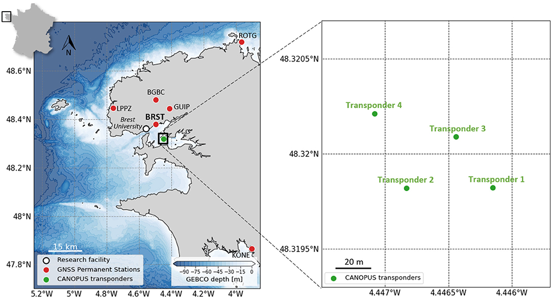
Figure 1. Study area. (Left) The Bay of Brest and the permanent GNSS network (red dots); (Right) Geographic locations of the transponders during the experiment.

FIGURE 2

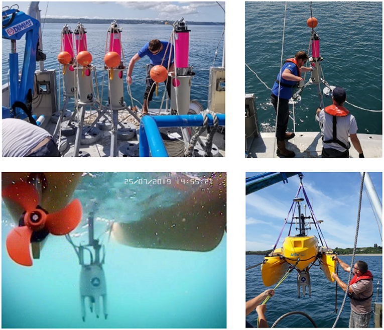
Figure 2. (Upper left and upper right) Preparation and deployment of the CANOPUS transponders mounted on tripods. The fourth one was not used in this study; (Lower left) iXblue integrated USBL/INS system (GAPS) mounted on PAMELi adjustable daggerboard; (Lower right) Deployment of PAMELi USV from R/V Albert Lucas. Note the installation of the GNSS antenna on the daggerboard, directly above the GAPS.

The CANOPUS transponders are omni-directional, and measure inter-transponder two-way travel times. This information can be used to measure relative displacements between transponders (e.g., Sakic et al., 2016; Lange et al., 2019; Petersen et al., 2019) or to constrain GNSS/A multi-transponder array positioning (e.g., Sweeney et al., 2005; Sakic et al., 2020). They can also communicate with the surface for telemetry or positioning purposes using an USBL or an acoustic modem. The transponders were equipped with temperature and pressure sensors, but this information was not used here, since we collected sound-speed profiles during the acquisition sessions. The transponder inclinometers showed that the tripods remained stable throughout the experiment.

2.2. The Surface Platform and Positioning Systems

An innovative aspect of this experiment was to mount the GNSS/A positioning system on an Unmanned Surface Vehicle (USV) named PAMELi (Plateforme Autonome Multicapteurs pour l'Exploration du Littoral—Autonomous Multisensor Platform for Coastal Exploration). The PAMELi project was developed by La Rochelle University for repeated and multidisciplinary monitoring of shallow coastal areas (Chupin et al., 2020). The vehicle, built by ASV, is a small battery-powered catamaran (3 m-long, 1.6 m-wide, weighting 300 kg), remotely controlled from a mother-ship or land through Wi-Fi, GSM, or VHF communications. Capable of cruising at 3–4 kn, it has an autonomy of about 8 h. Profiles can be pre-programmed or set-up interactively by remote control; in addition, with a propeller on each of its floats, the USV can maintain a stationary position within a radius given by the operator. Data from the mounted sensors can be telemetered to the operator and/or stored internally.

The GNSS receiver was a Spectra SP80, able to track and record signals from several GNSS constellations. The sampling rate was set at 1 Hz during the whole experiment. The Real-Time Kinematic (RTK) positioning mode was used to provide real-time positions to the GAPS system. The GNSS antenna was mounted directly above the underwater acoustic system on the keel of the USV (Figure 2).

The acoustic system was a GAPS (Global Acoustic Positioning System) M7 integrated USBL/INS device, manufactured by iXblue. Such devices are commonly used on oceanographic vessels for precise positioning of underwater devices or vehicles. The GAPS is a 64 cm-high and 30 cm-wide cylinder with four legs (Figure 2). The acoustic signal is emitted by a central acoustic head and received by an antenna made of four hydrophones ca. 21 cm apart. This design allows to measure both the two-way travel times and the direction of the return signal from the interrogated underwater device, here the transponders. In an optimal configuration, i.e., for a SNR ≥ 20 dB, the GAPS has a range accuracy of 2 cm and a bearing accuracy of 0.03°. The signal uses a frequency-shift keying modulation carried by a 26 kHz-signal. The GAPS is able to range every 0.8 s. For this experiment, it was configured to range the transponders every 2 s. Ship's motion are corrected for by the GAPS' inertial system (INS), which also filters out spurious real-time GNSS positions. This INS has an accuracy of 0.01° on the heading, roll and pitch components. With a GNSS receiver connected to the GAPS, vertical and horizontal displacements of the selected center of mass of the system (acoustic head or INS center) were thus fully constrained (pitch, roll, latitude, longitude, heading). The acoustic system, quasi weightless in sea-water, was immersed in the front of the USV, away from the propellers, at ~1m depth (Figure 2). Despite such keel, the USV remained very maneuverable, and operated smoothly in winds up to 12 kn. The GNSS and GAPS data acquisition were monitored in real-time from R/V Albert Lucas. The recorded noise was most of the time below 60 dB re μPa/$\sqrt{\text{Hz}}$, whereas, on a regular vessel, the noise would range between 70 and 85 dB.

2.3. Experimental Protocols

The GNSS/A experiment was carried out from July 23 to 25, 2019 in the Bay of Brest during the GEODESEA-2019 experiment (Royer et al., 2021). Its goals were (1) to test the CANOPUS transponders and their auxiliary sensors, and (2) to test the feasibility of GNSS/A positioning from an USV. The Bay of Brest provided a convenient area, close to port and sheltered from the open-sea swell. The nearest permanent GNSS station (BRST) was only 8 km away from the deployment area (see also section 3.2). Five vertical sound-velocity profiles were acquired during the experiment using a CTD probe. The profiles are shown in Figure 4. To avoid strong tidal currents, the experience took place during a neap tide period (coefficients 50 to 44)¹ and weather conditions were sunny and calm. The tides had a 2–3 m amplitude (i.e., the depth of the transponders varied by that amount about an average depth of 38 m).

During deployment, transponder TP#4 tipped over, but despite its transducer on the ground, operated at nominal capacity. Still, this transponder will not be considered here. For the absolute positioning test, three different acquisition protocols were tested (Figures 3, 4):

• In a Box-in mode, the USV navigated for about 20–30 min along repeated circles of 10 m diameter (about 1/4th the water depth) centered on the transponder of interest. Thus, the shooting angle w.r.t. to the vertical was ~12° and the average slant range was equal to the depth. The circles were traveled both clockwise and anti-clockwise;

• In a Static-above mode, the USV remained stationary for 10–15 min within a 3 m circle centered at the apex of the considered transponder;

• In a Static-slanted mode, the USV remained stationary during 1 h within a 3 m circle centered at the apex of the barycenter of the triangle made by the three vertical transponders. Acoustic rays were then slanted by about ~20°. In this mode, the GAPS ranged each transponder in turn.

FIGURE 3

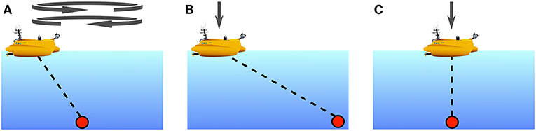
Figure 3. Different data acquisition modes: (A) Box-in, with clockwise and anti-clockwise circles around and centered on the transponder (red dot), (B) Static-slanted, and (C) Static-above the transponder.

FIGURE 4

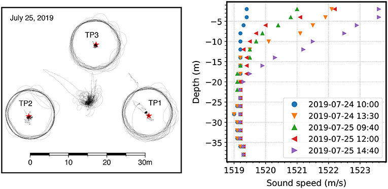
Figure 4. (Left) Data acquisition trajectories of the USV during Day 2, including box-in circles and stations above or slanted relative to the transponders (TP, red stars). (Right) Sound-speed profiles acquired during the experiment.

3. Data Processing

3.1. Inputs and Outputs

The ultimate objective of GNSS/A positioning is to determine the coordinates of seafloor transponders. For each transponder i, we note its coordinates X_Ri = [x_Ri, y_Ri, z_Ri]. We assume these coordinates fixed and stable during the whole experiment, since the transponders are installed on rigid and ballasted metal tripods. These coordinates will be derived from the following observations (represented in Figure 5):

• The positions of the embarked surface devices X_S = [x_S, y_S, z_S], provided by GNSS observations. Since the USV is moving, X_S is a function of time and thus we have, for each epoch t of the experiment, X_S(t). The embarked devices are, namely:

– the GNSS antenna whose position is X_GNSS(t).

– the GAPS acoustic head emitting the acoustic pings, whose position is X_AHD(t).

– and the GAPS four-hydrophones receiving the returned pings, whose positions are X_HPj(t), where j ∈ [[1, 4]].

• The tie vectors X_MEC (also known as lever arms), that link the different surface devices in the mechanical frame MEC of the USV. These vectors were measured manually on-shore before the USV deployment;

• The attitude of the USV, i.e., the heading α, pitch β, and roll γ angles recorded by the Inertial Motion Unit (IMU) integrated in the GAPS. So for each epoch t, R(t) = [α(t), β(t), γ(t)] is acquired;

• The two-way-travel times τ_i (called TWTT hereinafter) between the GAPS and the seafloor transponders for each acoustic ping i. Each TWTT is received at instant t_{TWTT, rec, i}. The emission instant t_{TWTT, emi, i} of the corresponding ping is determined by the relation t_{TWTT, rec, i} = t_{TWTT, emi, i}+τ_i + τ_TAT. The τ_TAT (for Turn Around Time) is a preset delay before the transponder replies to an interrogating signal. Since there are four hydrophones recording separately, for one emitted ping i, there are four TWTT values τ_i,_j and four distinct reception instants t_{TWTT, rec, i, j};

• The direction of arrival (also known as direction cosines, called DOA hereinafter), corresponding to the vectors between the GAPS and each transponder. Here, we used the DOA values directly estimated by the GAPS interface. In addition to the TWTTs, for each ping i, the DOA vector is defined as D_i = [d_{x, i}, d_{y, i}, d_{z, i}], which we assumed normalized;

• And a sound-speed profile (SSP) made of two vectors Z and C, respectively the depth and corresponding sound speed. Since this experiment took place in shallow waters over a short-time period, we here assumed that the sound velocity field was homogeneous (Sakic et al., 2018). From the sound-speed profile, an harmonic mean value can be determined: $c_{ref}=\frac{z_{max}-z_0}{{\int }_{z_0}^{z_{max}}c{(z)}^{-1}dz}$. This simplification allowed us to estimate a correction δc to this mean value. When processing each acquisition mode, described hereafter, we applied the nearest available SSP.

FIGURE 5

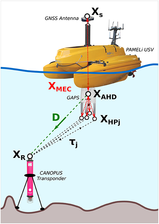
Figure 5. Components and vector representation of the GNSS/A system (description in section 3.1).

To simplify the calculations, the coordinates of the transponders will be determined in a local topocentric reference frame with North, East, and Down axes, hereafter called NED. We arbitrarily chose the NED frame origin [x₀, y₀, z₀] as the center of gravity of the three vertical transponder array.

3.2. GNSS Processing

To determine the GAPS position at the emission and reception times in a terrestrial reference frame, the GNSS position of the USV must be transferred to the acoustic system. During the experiment, the former was determined from real-time kinematic (RTK) positioning. Through the cellular network, the SP80 receiver downloaded the real-time corrections from the French TERIA network and achieved a centimetric positioning accuracy (Chambon, 2019). This method is commonly used in geodetic field experiments, whenever the RTK network is accessible. The transfer of accurate real-time positions from GNSS to the GAPS also allowed the INS to be realigned and limit the effects of the USV drift.

To test the quality of our RTK real-time positioning, the GNSS data were post-processed with the RTKLIB software, using the double-difference method (Takasu and Yasuda, 2009). We use the BRST permanent station as the reference base (Figure 1); this station, located at ~8 km from our working area, is part of the French permanent RGP-GNSS network managed by IGN (the French national mapping agency). Since real-time coordinates were given in the French national reference system RGF93 (Duquenne, 2018), for the sake of consistency, we computed all post-processed coordinates in this reference system. We considered the GPS data only (hereinafter called “GPS-only mode”), and all the available data including those of the Galileo and GLONASS constellations (hereinafter called “multi-GNSS mode”). In the absence of operational IGS multi-GNSS products so far (Mansur et al., 2020; Sośnica et al., 2020), we used the GFZ multi-GNSS products for orbit and clock corrections (Deng et al., 2017; Männel et al., 2020). The other GNSS processing parameters are summarized in Table 1.

TABLE 1

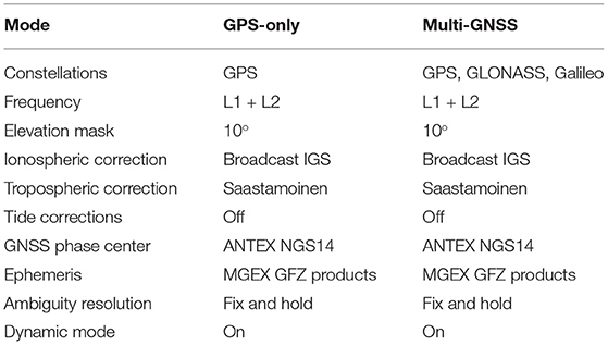
Table 1. GNSS post-processing parameters.

3.3. Transfer of the GNSS Position to the GAPS

The objective is to determine the GAPS position at the emission and reception instants. This is the reason why it is necessary to transfer the GNSS-antenna position to the different GAPS components (emitter and receivers).

The input data involved in this operation are:

• The positions of a main GNSS antenna in a global Earth-centered, Earth-fixed reference frame ECEF, either geocentric (x_i, y_i, z_i) or geographic (φ_i, λ_i, h_i), at sampling times t_{GNSS, i}. We call them X_{ECEF, GNSS}(t_{GNSS, i});

• The heading α, pitch β, and roll γ angles of the USV at the sampling time t_{INS, i};

• The tie vectors between these devices in the USV internal mechanical frame MEC. If we consider the GAPS IMU reference point as the origin of this frame, then X_{MEC, IMU} = [0, 0, 0]. The coordinates of the GNSS-antenna reference point (X_{MEC, GNSS}), that of the acoustic head (X_{MEC, AHD}) and those of the four hydrophones (X_{MEC, HPj}) are thus expressed with respect to the IMU reference point. To simplify the notation, X_{MEC, AHD} and X_{MEC, HPj} are hereinafter assimilated to the same vector X_{MEC, S}.

Thus, the objective is to get, in the NED topocentric reference frame, the coordinates of the GAPS (X_{NED, S}(t)) at the ping emission t_{emi, i} and reception t_{rec, i} instants. The USV position X_{ECEF, GNSS} is transferred into the NED frame using the formula described, for instance, by Grewal et al. (2007), and thus we have X_{NED, GNSS} for any sampling instant t_{GNSS, i}. We then performed a linear interpolation to obtain the exact positions of the platform at the ping emission and reception instants (t_{emi, i} and t_{rec, i}).

Meanwhile, the USV on-board device coordinates in the MEC frame are transferred to the “instantaneous topocentric frame” iNED. It corresponds to a transformation of the MEC frame where its axes are co-linear to the NED ones, i.e., by applying the USV attitude R to the tie vectors. To do so, we associated a quaternion q(t_{INS, i}) to each record of the IMU, R(t_{INS, i}) (Großekatthöfer and Yoon, 2012). We renamed t_i the instants t_{emi, i} and t_{rec, i} since the procedure is the same for the emission and reception instants. Then, using the Slerp attitude interpolation method (Kremer, 2008), we determine the attitude of the platform at instant t_i represented by the quaternion q_i.

From this operation, the positions of the GNSS and of the GAPS acoustic head and hydrophones in the iNED frame at the transmission and reception instants are determined by:

$\begin{array}{ll}{\text{X}}_{iNED,S}(t_i)={\text{q}}_i\left[\begin{array}{c}0\\ {\text{X}}_{MEC,S}(t_i)\end{array}\right]{\text{q}}_i^{-1}& (1)\end{array}$

$\begin{array}{ll}{\text{X}}_{iNED,GNSS}(t_i)={\text{q}}_i\left[\begin{array}{c}0\\ {\text{X}}_{MEC,GNSS}(t_i)\end{array}\right]{\text{q}}_i^{-1}& (2)\end{array}$

It comes that the vector T_i between the iNED positions of the GNSS and the GAPS is:

$\begin{array}{ll}{\text{T}}_i=\overrightarrow{GNSS,S}={\text{X}}_{iNED,S}-{\text{X}}_{iNED,GNSS}& (3)\end{array}$

Then, the NED position of the GNSS can be transferred to the GAPS by translation:

$\begin{array}{ll}{\text{X}}_{NED,S}(t_i)={\text{X}}_{NED,GNSS}(t_i)+{\text{T}}_i& (4)\end{array}$

3.4. Least-Squares Model

Finally, we used a least-squares (LSQ) inversion (e.g., Strang and Borre, 1997; Ghilani, 2011) to estimate the desired parameters, namely the transponder coordinates X_Ri and the sound speed correction δc. The observable, in the least-squares sense, are the TWTTs τ_i and the DOAs D_i. Thus, the associated observation functions f_TWTT and f_DOA are:

$\begin{array}{ll}{f}_{TWTT}:({\text{X}}_R,\delta c)\mapsto \tau & (5)\end{array}$

$\begin{array}{ll}{f}_{DOA}:({\text{X}}_R)\mapsto \text{D}& (6)\end{array}$

We have:

$\begin{array}{ll}{f}_{TWTT}:\frac{{\Vert \text{X}}_R-{\text{X}}_{AHD}(t_{emi})\Vert +\Vert {\text{X}}_R-{\text{X}}_{HPj}(t_{rec})\Vert }{c+\delta c}+{\tau }_{TAT}=\tau & (7)\end{array}$

$\begin{array}{ll}{f}_{DOA}:\frac{{\text{X}}_R-{\text{X}}_{AHD}(t_{rec})}{\Vert {\text{X}}_R-{\text{X}}_{AHD}(t_{rec})\Vert }=\text{D}& (8)\end{array}$

To establish the Jacobian matrix A, we need the partial derivatives of f_TWTT and f_DOA:

$\begin{array}{ll}\frac{\partial f_{TWTT}}{\partial {\text{X}}_R}=\frac{1}{c+\delta c}·\left(\frac{{\text{X}}_R-{\text{X}}_{AHD}(t_{emi})}{\Vert {\text{X}}_R-{\text{X}}_{AHD}(t_{emi})\Vert }+\frac{{\text{X}}_R-{\text{X}}_{HPj}(t_{rec})}{\Vert {\text{X}}_R-{\text{X}}_{HPj}(t_{rec})\Vert }\right)& (9)\end{array}$

$\begin{array}{ll}={\left[\begin{array}{c}\frac{1}{c+\delta c}·\left(\frac{x_R-x_{AHD}(t_{emi})}{\Vert {\text{X}}_R-{\text{X}}_{AHD}(t_{emi})\Vert }+\frac{x_R-x_{HPj}(t_{rec})}{\Vert {\text{X}}_R-{\text{X}}_{HPj}(t_{rec})\Vert }\right)\\ \frac{1}{c+\delta c}·\left(\frac{y_R-y_{AHD}(t_{emi})}{\Vert {\text{X}}_R-{\text{X}}_{AHD}(t_{emi})\Vert }+\frac{y_R-y_{HPj}(t_{rec})}{\Vert {\text{X}}_R-{\text{X}}_{HPj}(t_{rec})\Vert }\right)\\ \frac{1}{c+\delta c}·\left(\frac{z_R-z_{AHD}(t_{emi})}{\Vert {\text{X}}_R-{\text{X}}_{AHD}(t_{emi})\Vert }+\frac{z_R-z_{HPj}(t_{rec})}{\Vert {\text{X}}_R-{\text{X}}_{HPj}(t_{rec})\Vert }\right)\end{array}\right]}^{⊺}& (10)\end{array}$

$\begin{array}{ll}\frac{\partial f_{TWTT}}{\partial \delta c}=\frac{-\Vert {\text{X}}_R-{\text{X}}_{AHD}(t_{emi})\Vert -\Vert {\text{X}}_R-{\text{X}}_{HPj}(t_{rec})\Vert }{{(c+\delta c)}^2}& (11)\end{array}$

$\begin{array}{l}\frac{\partial f_{DOA}}{\partial {\text{X}}_R}=\\ \left[\begin{array}{ccc}-\frac{{(y_R-y_S)}^2+{(z_R-z_S)}^2}{{\Vert {\text{X}}_R-{\text{X}}_{AHD}(t_{rec})\Vert }^3}& -\frac{(x_R-x_S)(y_R-y_S)}{{\Vert {\text{X}}_R-{\text{X}}_{AHD}(t_{rec})\Vert }^3}& -\frac{(x_R-x_S)(z_R-z_S)}{{\Vert {\text{X}}_R-{\text{X}}_{AHD}(t_{rec})\Vert }^3}\\ -\frac{(y_R-y_S)(x_R-x_S)}{{\Vert {\text{X}}_R-{\text{X}}_{AHD}(t_{rec})\Vert }^3}& -\frac{{(x_R-x_S)}^2+{(z_R-z_S)}^2}{{\Vert {\text{X}}_R-{\text{X}}_{AHD}(t_{rec})\Vert }^3}& -\frac{(y_R-y_S)(z_R-z_S)}{{\Vert {\text{X}}_R-{\text{X}}_{AHD}(t_{rec})\Vert }^3}\\ -\frac{(z_R-z_S)(x_R-x_S)}{{\Vert {\text{X}}_R-{\text{X}}_{AHD}(t_{rec})\Vert }^3}& -\frac{(z_R-z_S)(y_R-y_S)}{{\Vert {\text{X}}_R-{\text{X}}_{AHD}(t_{rec})\Vert }^3}& -\frac{{(x_R-x_S)}^2+{(y_R-y_S)}^2}{{\Vert {\text{X}}_R-{\text{X}}_{AHD}(t_{rec})\Vert }^3}\end{array}\right]& (12)\end{array}$

Then, the problem is solved with an approach similar to the one described by Sakic et al. (2020). The adjustment δX on the a priori values X₀ of the transponder coordinates and the sound speed correction are given by the relation:

$\begin{array}{ll}\delta \text{X}={({\text{A}}^{⊺}\text{P B})}^{-1}{\text{A}}^{⊺}\text{P B}& (13)\end{array}$

where A is the Jacobian in the neighborhood of X₀. B and P is the weight matrix. If the DOA are ignored, P is equal to the identity and corresponds to the differences between the observations and the theoretical quantities determined by f_TWTT(X₀) and f_DOA(X₀). In the end, the observation residuals are given by:

$\begin{array}{ll}\text{V}=\text{B}-\text{A}({\text{X}}_0+\delta \text{X})& (14)\end{array}$

Since the algorithm needs several steps k to converge, we used an iterative process where the estimated values become the new a priori values at step k+1, so that _{X0, k}+δX_k =_{X0, k+1}. The iterations stop when the convergence criterion is met, in our case when ${\delta \mathbf{\text{X}}}_k<10^{-5}m$. It generally occurs after the fourth or fifth iteration.

3.5. Outlier Detections

To eliminate the outliers, both in the TWTTs and the DOAs, we use the MAD (Median Absolute Deviation) method (Leys et al., 2013).

For a set of observation L, the MAD is defined as:

$\begin{array}{ll}MAD=median(|\text{L}-median(\text{L})|)& (15)\end{array}$

Then, for each observation l_i (where l_i ∈ {τ_i, d_{x, i}, d_{y, i}, d_{z, i}}), we have M_i so as :

$\begin{array}{ll}{M}_i=\frac{b(l_i-median(\text{L}))}{MAD}& (16)\end{array}$

where b is a coefficient related to the statistical distribution of the data considered (Rousseeuw and Croux, 1993). If the distribution is normal, b ≈ 0.67449. Then, if M_i > s, l_i is eliminated as an outlier for the next iteration, s is a threshold and typically we take s = 3 if the distribution is normal.

4. Data Analysis

4.1. Parameterization

The data acquired during the experiment were processed with the model described in the previous sections. The observed TWTTs were weighted by an a priori standard deviation ς_TWTT = 2 × 10⁻⁵ s, corresponding to the time precision described in the GAPS data-sheet. We tested different configurations where the sound-speed correction δc is estimated and where it is not. We also tested the contribution of the DOAs in the precision and repeatability of the transponder position. We thus processed the DOAs in three different ways: (1) not used in the inversion, (2) taken into account with a loose a priori standard deviation ς_{DOA, l} = 10⁻² or (3) considered as fully constraint ς_{DOA, c} = 10⁻³. Like the DOAs, ς_DOA are unitless and were chosen based on the direction cosine variations for signal's direction of arrival uncertainties δθ at ≈45°. For δθ = 1 and 0.1°, we found ${\varsigma }_{DOA}=cos(45\bullet +\delta \theta )-cos(45\bullet )\approx 10^{-2}$ and 10⁻³, respectively.

4.2. Test of Different Parameterizations in a Box-In Mode

To test whether the DOAs improve the positioning accuracy, we first exploited the observations made in box-in modes on Day 2. As we focused on the acoustic positioning algorithm, we used the post-processed GPS-only data as the surface positioning solution. We processed each box-in with the six parameterizations described in section 4.1, made up of three ς_DOA and two δc modes (estimated or not). The acquisition duration were in the order of ~25 min, as summarized in Table 2A along with the number of recorded TWTTs and the percentage of TWTT outliers.

TABLE 2

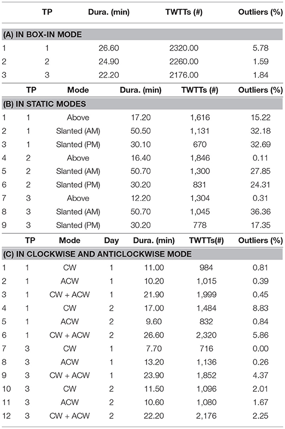
Table 2. Acquisition duration, number of pings, and percentage of outlier pings for each transponder in the different acquisition modes.

When errors are independent from epoch to epoch and follow a Gaussian distribution, having more data will reduce the final position error. However, noise in GNSS positioning is known to be colored (Williams, 2004), and the ocean properties, such as current, salinity, or temperature, do not evolve with a white noise either. Therefore, subsampling the data from the experiment may give results that are highly sensitive to the selected subsampled windows. To test the accuracy (or appropriateness) of the model used in the least-squares inversion, we extracted successive and non-overlapping subsets from the experimental dataset and observed how the resulting transponder position changed between subsets. We can then derive a standard deviation for each parameterization. For each transponder, we divided the total acquisition period into five data subsets, each containing the same number of USV circles around the transponder.

Figure 6 shows the resulting locations for the three transponders. Each parameterization is represented in a different color and symbol. The “tripod” symbols (, , ) represent runs where the δc estimation is disabled, and the triangles (▸, ▴, ▾) represent runs where δc is estimated. The light tripods and empty triangles represent the LSQ inversion result for each of the five data subsets, and the bold/thick equivalent symbols represent the arithmetic mean of the five subsets, with their standard deviations. Star filled-symbols (★) in matching colors represent the results of the LSQ inversion for the entire period, with their formal standard deviation. Standard deviations for each parameterization are listed in Table 3.

FIGURE 6

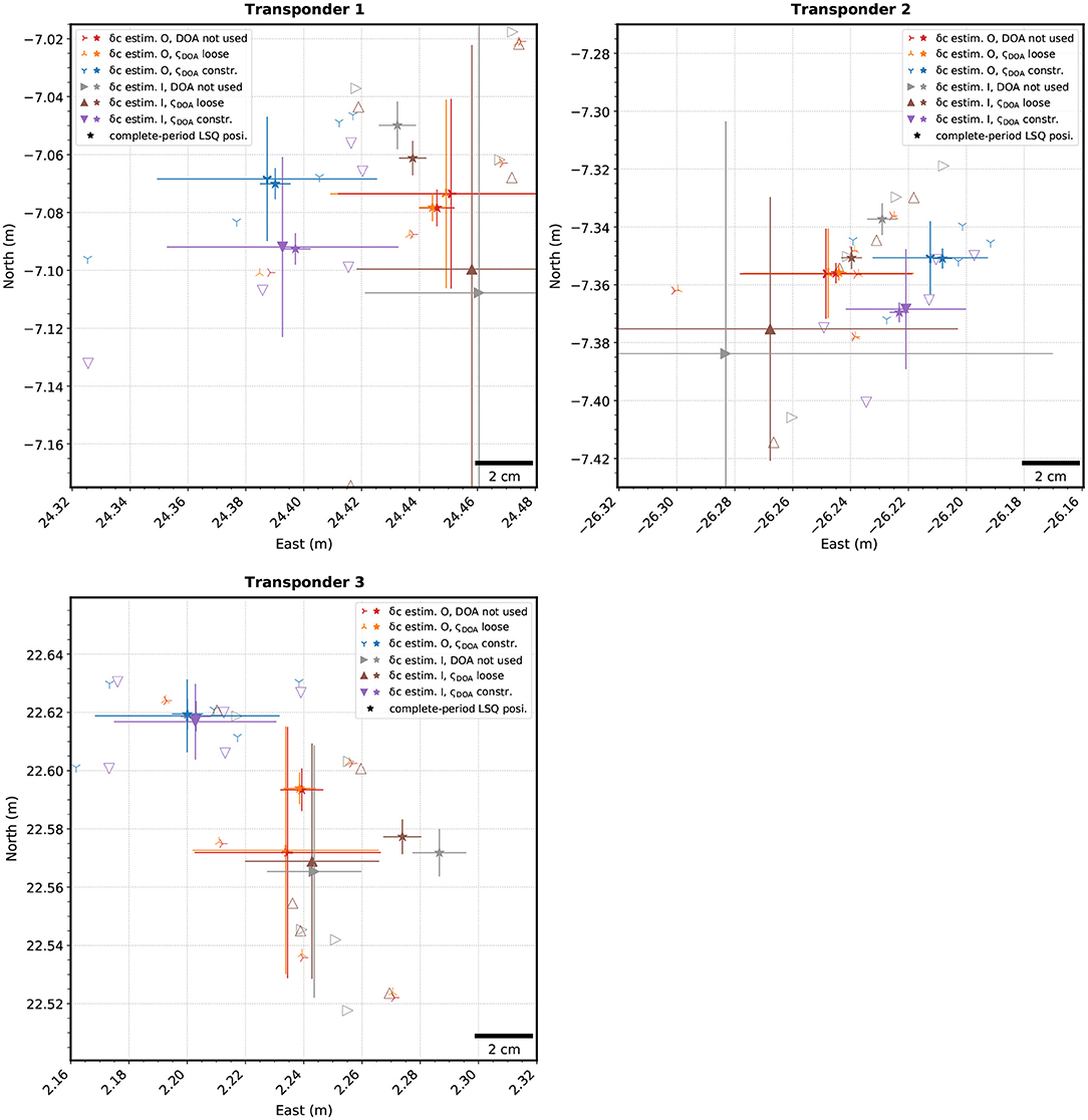
Figure 6. Positions of the three transponders based on the box-in acquisitions, in a local topocentric reference frame. The thin tripod symbols (, , ) and empty triangles (P, △, ▽) represent the LSQ inversion results for each of the five data subsets. The equivalent bold/thick symbols represent the arithmetic means of the five subset-derived positions with their standard deviations. The colored-star (★) represents the result of the LSQ inversion and its formal standard deviation, based on the entire dataset; colors correspond to the different parameterizations used. For the δc estimation, “I” stands for used, and “O” for not used. Few outlier solutions are outside the frame.

TABLE 3

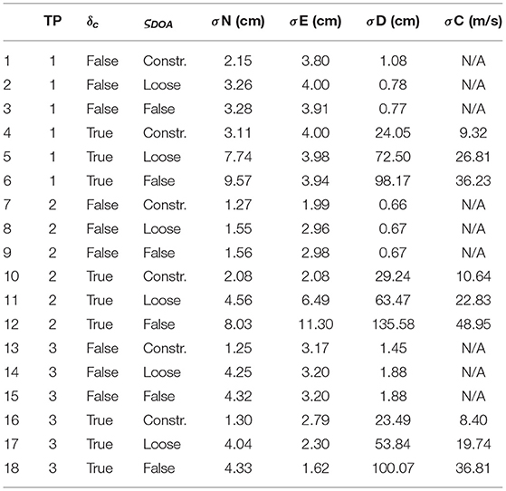
Table 3. Standard deviations of the North, East, Depth, and Celerity components, for each parameterizations (δ_c and ς_DOA columns) and each transponders (TP column) in box-in mode.

First of all, solutions where δc is estimated and DOAs are not used or loosely constrained (▸ and ▴) yield high standard deviations and a poor compatibility with their complete period counterpart. This is due to a complete trade-off between the TWTTs and the sound speed. Such parameterization should thus be avoided. Solutions where δc is not estimated while the DOAs are either unused or loosely constrained ( and ) give almost equal values (within a millimeter). In a box-in mode, we can conclude that using loose or no constraints from the DOAs yields equivalent results, if δc is not estimated. It is worth noting that when DOAs are constrained ( and ▾), standard deviations are smaller compared to the two previous solutions. However, compatibility with the solution based on the whole period is also smaller, which shows the best stability among these parameterizations.

When DOAs are constrained, we note a difference for transponders 1 and 3 between solutions whether δc is estimated or not, even if the subset standard deviations are slightly higher when δc is estimated. This dispersion may be due to the relatively small number of TWTTs in each data subset (~440), which prevents a reliable estimation of the δc parameter. Nevertheless, the residual sum of squares remains smaller by about 2–10% (which is expected since adjusting an additional parameter reduces the residuals). Thus, in a box-in mode, a solution with constrained DOAs and estimated δc is considered as the most optimal parameterization.

Note that even if the horizontal standard deviation is mostly below 10 cm, the standard deviation on the depth can reach the meter level. This is due to the high dependence of depth on sound velocity. Nevertheless, the parameterization with constrained DOAs and estimated δc also tends to reduce the dispersion on the vertical component.

4.3. Repeatability in Static Mode

The repeatability of the different parameterizations in a static mode can be evaluated from the data collected Day 2, where two sessions in a static-slanted mode were recorded, in the morning (AM) and in the afternoon (PM) (Figure 3B), along with a station above each transponder (Figure 3C). Table 2B summarizes the acquisition sessions, the number of recorded TWTTs and the outlier ratio. The results are presented in Figure 7 and Table 4.

FIGURE 7

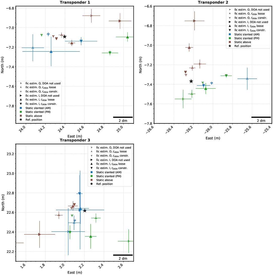
Figure 7. Positions of the three transponders based on the static acquisitions. The symbols represent the different parameterizations and the colors the acquisition modes (static-slanted in the morning or the afternoon, and static-above). The horizontal and vertical bars are LSQ formal standard deviations. The black stars (★) represent the real-time solutions provided by the USBL/INS system after box-in (see section 4.2). For δc estimation, “I” stands for used, and “O” for not used. Few outlier solutions are outside the frame.

TABLE 4

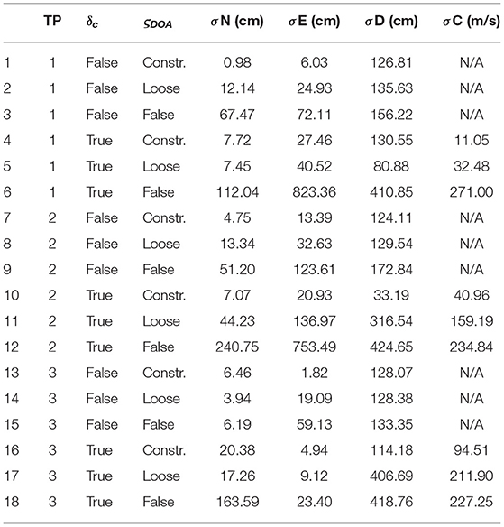
Table 4. Standard deviations of the North, East, Depth, and Sound-speed components, for each parameterizations (δ_c and ς_DOA columns) and each transponders (TP column) in static modes.

The three sub-figures in Figure 7 show the resulting locations for the three transponders in static mode. Symbols represent different parameterizations and colors, different static acquisition modes. The horizontal and vertical bars give the LSQ formal standard deviations. The black star (★) shows the position estimated from the box-in mode in section 4.2.

Parameterizations where δc is estimated and DOAs are loosely constrained yield a repeatability of several decimeters between the three sessions, up to a meter when DOAs are not used and δc is estimated. The dispersion of the solutions decreases depending on whether DOAs are not used, loosely or fully constrained, showing that taking DOAs into account improves the position determination. The best repeatability is obtained with constrained DOAs but δc not estimated. The dispersion then ranges between 1 and 6.5 cm on the North component and 6 and 13.4 cm on the East component. Moreover, these solutions are the most consistent with the best solution obtained in a box-in mode (section 4.2). The dispersion with constrained DOAs is two to three times greater when estimating δc. Thus, in a static mode, estimating the sound speed is not optimal, as it does not improve the solution. Moreover, the solutions without DOAs are constrained only by the small USV displacements induced by the waves and the currents (a perfectly still USV on a perfectly flat sea would lead to a singular design matrix and thus to an under-determined problem). In general, a static acquisition is not optimal for geodetic applications due to the lack of constrain on the vertical component in the USV motion; the addition of a depth sensor (echosounder or pressure sensor) would be needed.

4.4. Repeatability of Box-In Mode

To further test the repeatability of the box-in mode, we compared the sessions between Day 1 and 2, and particularly the effects of the USV direction when circling the transponders. Thus, we processed separately, for both days and for transponders 1 and 3, periods when the USV was rotating clockwise (CW) or anticlockwise (ACW), and when clockwise + anticlockwise (CW + ACW) acquisitions were combined (Table 2C and Figure 8). Unfortunately, the raw GNSS observations are not available for the first day (and thus could not be reprocessed), so all these tests use the Real-Time RTK positions of the USV.

FIGURE 8

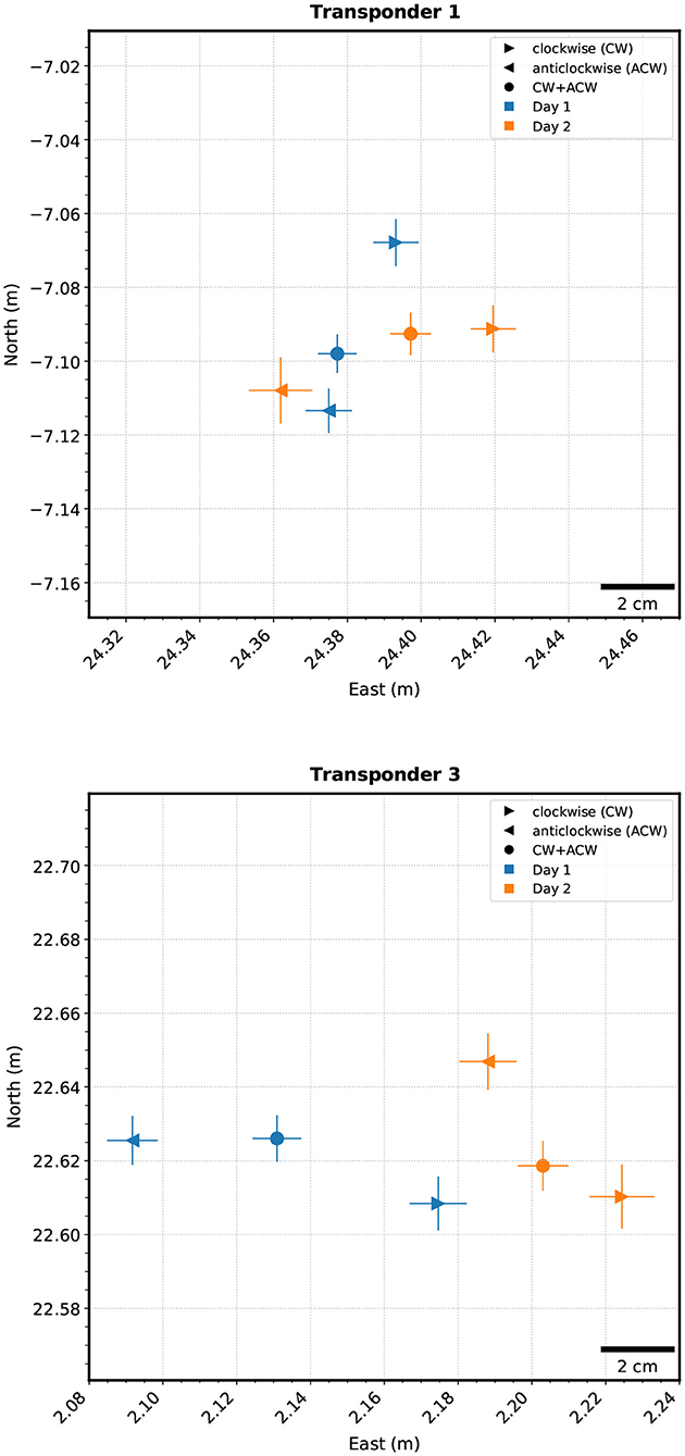
Figure 8. Positions of transponders 1 and 3 based on a clockwise box-in (▸) and anticlockwise box-in (◂) for Day 1 and 2, compared to the result combining CW and ACW box-ins (•).

Despite the short duration of each session, the results display a very good repeatability between Days 1 and 2 for the combined CW + ACW sessions (Table 5B). The differences are smaller than 3 cm on the North and East components, except for Transponder 3 which shows a difference of 7.2 cm on the East component. This difference could be explained by the poor repeatability of the ACW rotation. As expected, the CW + ACW solution is located in the middle of the individual CW and ACW solutions. It is also worth noticing that the rotation direction seems to influence the repeatability of the box-in (Table 5A). The horizontal difference is about 5 cm, and up to 8.5 cm for transponder 3 on Day 1. This difference may be due to changes in the water column between successive CW and ACW acquisitions or to an unidentified bias in the lever arms; both effects would averaged out in combining CW and ACW sessions.

TABLE 5

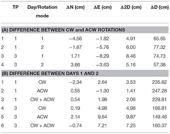
Table 5. (A) Differences on East, North, and Down components between clockwise and anti-clockwise box-in rotations. (B) Differences in the East, North, and Down components between days 1 and 2 for clockwise (CW), anti-clockwise (ACW), and complete (CW + ACW) box-in circles.

4.5. Influence of the GNSS Solution on Seafloor Positioning

To evaluate the effects of GNSS positioning (section 3.2), namely real-time RTK, GPS-only and multi-GNSS, on the overall solution, we analyzed the TWTT residuals after the least-square inversion. We considered the three transponder box-in modes presented in section 4.2 and tested the three different GNSS solutions. The inversion is based on constrained DOAs and an adjusted δc. The results are shown in Figure 9 and Table 6. For a better readability, the TWTT residuals are converted into distances using the estimated sound speed.

FIGURE 9

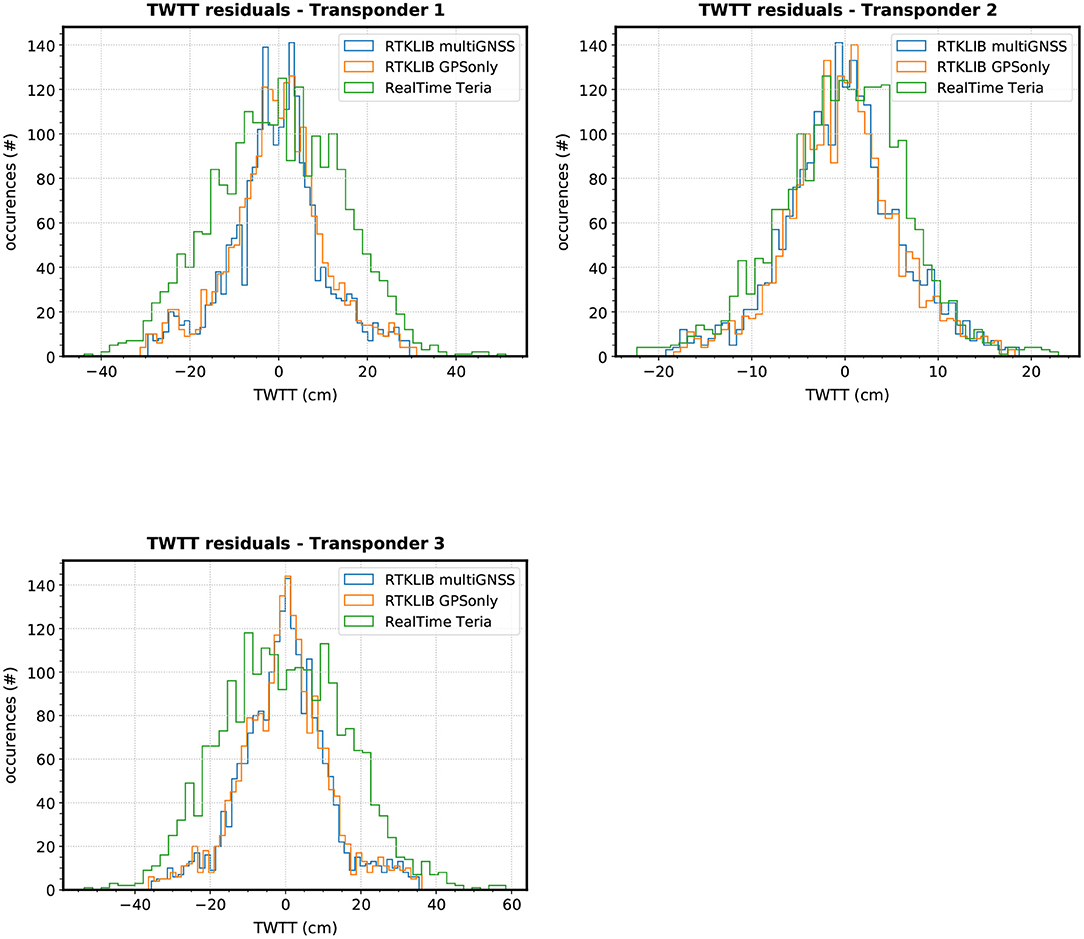
Figure 9. Histograms of the TWTT residuals (converted to distance) based on the different GNSS solutions for the three transponders in box-in mode.

TABLE 6

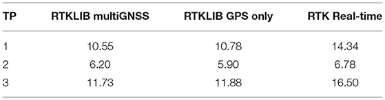
Table 6. Standard deviation in centimeters of the TWTT residuals converted to distance using different GNSS solution type for the three transponders (TP) in box-in mode.

We can see that the GNSS solution has an effect on the TWTT residuals. The standard deviation difference for transponders 1 and 3 are respectively ~3.5 and ~4.5 cm smaller for post-processed solution compared to the real-time one. The multi-GNSS solution also yields slightly smaller residuals than the GPS-only solution but the improvement is not significant. For transponder 2, the post-processed vs. real-time difference is less prominent (~5 mm) and the GPS-only solution gives smaller residuals. Overall, the post-processed solutions provide smaller TWTT residuals than the real-time solution.

5. Discussion

In line with previous experiments (Chadwell et al., 2016; Iinuma et al., 2021), this study confirms the feasibility of GNSS/A positioning from an USV. In addition to an easier implementation at a reduced cost, the size of USV avoids any complex topometric survey to determine the lever arms of the system (eg. Chadwell, 2003). Here, the lever arms were measured directly on-shore with a simple ruler with an optimal accuracy. Nevertheless, an a posteriori adjustment of the lever arms in the LSQ model can be valuable (Chen et al., 2019). Regarding the absolute positioning, we used a simple linear interpolation to determine the USV's position at the ping emission and reception epochs. This approach is sufficient for the static modes since the GNSS position sampling rate is high (1 Hz) and the USV displacements relatively small (sub-meter level). Nevertheless, a Lagrangian interpolation would be more appropriate when the USV is moving (box-in mode).

USV platforms may revolutionize seafloor geodesy in the near future. In addition to more frequent and spatially denser GNSS/A observations, combining multiple platforms (USVs and a ship) can allow a simultaneous monitoring of the sound-speed field in the ocean (Matsui et al., 2019; Ishikawa et al., 2020). This parameter undoubtedly remains the most critical for an accurate underwater geodetic positioning.

Using an USBL (here a GAPS) instead of a simple acoustic modem allow to measure DOAs in addition to TWTTs. Integrating these observations in the least-squares inversion improve the transponder positioning accuracy. We have shown that, both in box-in and static acquisitions, taking the DOAs into account improves the repeatability of the estimated positions between different sessions.

This experiment in shallow water (~40 m) is a proof-of-concept. The repeatability of the sessions in box-in mode is about 5 cm. Such accuracy is not sufficient to measure plate motions or fault-slips which are in the order of few mm/year to cm/year (e.g., Bürgmann and Chadwell, 2014), unless measurements are repeated very often and over half a decade or more. Despite the significant contribution of the DOAs, longer acquisition sessions (i.e., continuous over few hours) would be necessary in a true experiment. The effect would be to average out the GNSS positioning and acoustic propagation errors along with internal wave effects. Moreover, the poor repeatability of static acquisitions clearly shows that additional observations like depth are required to efficiently estimate the sound speed.

Since the DOA accuracy is a function of the water depth, DOAs in deep waters may not be as critical as in shallow waters for the precision of seafloor positioning. Further investigations are needed to assess their actual contribution in the deep ocean. In any case, one of the objectives of this work was to explore the contribution of such information, and we believe that DOAs would improve seafloor positioning accuracy, for instance, in an experiment using a single seafloor transponder and several ranging mobile-platforms. They could also be of value to observe fast and/or repeated co-seismic displacements of the seafloor (in the order of several centimeters within few days), where active tectonics occurs in shallow waters, as for instance, off the Vanuatu Islands (e.g., Ballu et al., 2013) or near the Saintes Archipelago (West Indies) (e.g., Bazin et al., 2010).

In this paper, we chose to adjust the sound speed by a simple constant since the acquisition sessions were short (15 min to 1 h). The sound speed variability between the beginning and end of a session could thus be neglected at first approximation. However, for longer sessions, adjusting this parameter with a sine, polynomial, or spline function should be preferred (Fujita et al., 2006; Yasuda et al., 2017; Chen et al., 2018; Liu et al., 2019). Moreover, in deeper waters, more accurate ray-tracing should also replace the straight-ray approximation (Chadwell and Sweeney, 2010; Sakic et al., 2018).

6. Conclusion

This experiment in the Bay of Brest, France, was meant to be a proof-of-concept for underwater geodetic positioning from an Unmanned Surface Vehicle. The experimental set-up comprised three acoustic transponders on the seafloor and an integrated USBL/INS system coupled with a GNSS receiver mounted on a USV. The locations of the transponders were derived from the recorded two-way-travel times between the USV and the transponders, and from the direction of arrival of the returned signals. The GNSS receiver, supplemented by the inertial system, provided the surface positioning. During the experiment and this study, different acquisition trajectories were compared: box-in circles and stations above or slanted relative to the transponders.

This paper describes a method to calculate the position of the USBL acoustic head from GNSS observations and attitude measurements. A least-squares model is developed to determine the transponder positions from TWTT and DOA observations, and from an estimation of the acoustic signal propagation speed. Using DOAs improve the repeatability of transponder positioning in box-in and static acquisitions. For a single transponder localization, box-in provides better results than a static acquisition. Over all the sessions spanning 2 days, the resulting repeatability of positioning is 5 cm, despite the short duration of the GNSS/A sessions (~20 min each). We also demonstrated a smaller dispersion of TWTTs residuals when a post-processed GNSS solution is used instead of the real-time RTK solution. This work could set the basis for operational USV-based GNSS/A campaigns for geophysical monitoring in the near future.

Data Availability Statement

The datasets used in this study can be found in the SEANOE database (www.seanoe.org/data/00674/78593/, doi: 10.17882/78593. Python 3 source codes developed for this article are freely available at an online GitHub git repository upon request to the corresponding author.

Author Contributions

J-YR and VB conceived, organized, and conducted the experiment. J-YR, VB, TC, MB, CC, P-YM, and PU participated to the data acquisition at sea. PS, VB, and CC elaborated the processing strategy. PS designed and implemented the model, and produced the results. CC post-processed the GNSS data and pre-processed the acoustic data. TC was in charge for setting-up and piloting the USV PAMELi. MB designed the transponder lay-out and acquired the sound-speed profiles. P-YM and PU provided the advice and expertise on the GAPS and CANOPUS transponders. J-YR, VB, PS, CC, P-YM, and PU discussed the results, contributed to, and edited the article. All authors contributed to the article and approved the submitted version.

Funding

The CANOPUS transponders were funded by the ERC FOCUS project (2019-2023, PI M.-A. Gutscher at LGO). This GNSS/A experiment (GEODESEA-2019) was funded by the French Oceanographic Fleet, LGO, and LIENSs, with support from the iXblue company for the preparation of the transponders and the implementation of their equipment. Funding for CC's Ph.D. was provided by the Direction Générale de l'Armement (DGA) and the Nouvelle Aquitaine Region.

Conflict of Interest

The authors declare that the research was conducted in the absence of any commercial or financial relationships that could be construed as a potential conflict of interest.

Acknowledgments

The authors would like to thank Charles Poitou (LGO) for his assistance in the deployment and recovery of the equipment. The authors also wish to thank the crew, Frank Quéré and Robin Carlier, of R/V Albert Lucas, LGO's director Marc-André Gutscher for the scientific and administrative support, and the iXblue team members Yoann Caudal and Corinne Le Guicher.

Supplementary Material

The Supplementary Material for this article can be found online at: https://www.frontiersin.org/articles/10.3389/feart.2021.636156/full#supplementary-material

Footnote

1. ^The French Navy's hydrographic and oceanographic service (SHOM) defines the amplitude of the tides for the French coasts on a scale ranging from 20 to 120.

References

Ballu, V., Bonnefond, P., Calmant, S., Bouin, M.-N., Pelletier, B., Laurain, O., et al. (2013). Using altimetry and seafloor pressure data to estimate vertical deformation offshore: Vanuatu case study. Adv. Space Res. 51, 1335–1351. doi: 10.1016/j.asr.2012.06.009

CrossRef Full Text | Google Scholar

Bazin, S., Feuillet, N., Duclos, C., Crawford, W., Nercessian, A., Bengoubou-Valérius, M., et al. (2010). The 2004–2005 Les Saintes (French West Indies) seismic aftershock sequence observed with ocean bottom seismometers. Tectonophysics 489, 91–103. doi: 10.1016/j.tecto.2010.04.005

CrossRef Full Text | Google Scholar

Berger, J., Laske, G., Babcock, J., and Orcutt, J. (2016). An ocean bottom seismic observatory with near real–time telemetry. Earth Space Sci. 3, 68–77. doi: 10.1002/2015EA000137

CrossRef Full Text | Google Scholar

Bürgmann, R., and Chadwell, D. (2014). Seafloor geodesy. Annu. Rev. Earth Planet. Sci. 42, 509–534. doi: 10.1146/annurev-earth-060313-054953

CrossRef Full Text | Google Scholar

Chadwell, C. D. (2003). Shipboard towers for global positioning system antennas. Ocean Eng. 30, 1467–1487. doi: 10.1016/S0029-8018(02)00141-5

CrossRef Full Text | Google Scholar

Chadwell, C. D., and Sweeney, A. D. (2010). Acoustic ray-trace equations for seafloor geodesy. Mar. Geod. 33, 164–186. doi: 10.1080/01490419.2010.492283

CrossRef Full Text | Google Scholar

Chadwell, C. D., Webb, S. C., and Nooner, S. L. (2016). “Campaign-style GPS-acoustic with wave gliders and permanent seafloor benchmarks,” in Proceedings of the Subduction Zone Observatory Workshop (Boise, ID: Boise Center).

Chambon, P. (2019). Du NRTK vers le PPP-RTK, un exemple avec TERIA. XYZ J. French Topogr. Assoc. 159, 44–49.

Chen, G., Liu, Y., Liu, Y., Tian, Z., Liu, J., and Li, M. (2019). Adjustment of transceiver lever arm offset and sound speed bias for GNSS-acoustic positioning. Rem. Sens. 11, 1–12. doi: 10.3390/rs11131606

CrossRef Full Text | Google Scholar

Chen, H. Y., Ikuta, R., Lin, C. H., Hsu, Y. J., Kohmi, T., Wang, C. C., et al. (2018). Back-arc opening in the western end of the Okinawa trough revealed from GNSS/acoustic measurements. Geophys. Res. Lett. 45, 137–145. doi: 10.1002/2017GL075724

CrossRef Full Text | Google Scholar

Chupin, C., Ballu, V., Testut, L., Tranchant, Y. T., Calzas, M., Poirier, E., et al. (2020). Mapping sea surface height using new concepts of kinematic GNSS instruments. Rem. Sens. 12:2656. doi: 10.3390/rs12162656

CrossRef Full Text | Google Scholar

Deng, Z., Nischan, T., and Bradke, M. (2017). Multi-GNSS Rapid Orbit-, Clock- and EOP-Product Series. doi: 10.5880/GFZ.1.1.2016.003

CrossRef Full Text | Google Scholar

Duquenne, F. (2018). Les systèmes de référence terrestre et leurs réalisations Cas des territoires français. XYZ J. French Topogr. Assoc. 154, 46–54.

Foster, J. H., Ericksen, T. L., and Bingham, B. (2020). Wave glider–enhanced vertical seafloor geodesy. J. Atmos. Ocean. Technol. 37, 417–427. doi: 10.1175/JTECH-D-19-0095.1

CrossRef Full Text | Google Scholar

Fujita, M., Ishikawa, T., Mochizuki, M., Sato, M., Toyama, S., Katayama, M., et al. (2006). GPS/Acoustic seafloor geodetic observation: method of data analysis and its application. Earth Planets Space 58, 265–275. doi: 10.1186/BF03351923

CrossRef Full Text | Google Scholar

Gagnon, K., Chadwell, C. D., and Norabuena, E. (2005). Measuring the onset of locking in the Peru-Chile trench with GPS and acoustic measurements. Nature 434, 205–208. doi: 10.1038/nature03412

PubMed Abstract | CrossRef Full Text | Google Scholar

Ghilani, C. (2011). Adjustment computations: spatial data analysis. Int. J. Geograph. Inform. Sci. 25, 326–327. doi: 10.1080/13658816.2010.501335

CrossRef Full Text | Google Scholar

Grewal, M. S., Weill, L. R., and Andrews, A. P. (2007). Global Positioning Systems, Inertial Navigation, and Integration. Hoboken, NJ: John Wiley and Sons, Inc.

Google Scholar

Großekatthöfer, K., and Yoon, Z. (2012). Introduction Into Quaternions for Spacecraft Attitude Representation. Berlin: TU Berlin.

Iinuma, T., Kido, M., Ohta, Y., Fukuda, T., Tomita, F., and Ueki, I. (2021). GNSS-acoustic observations of seafloor crustal deformation using a wave glider. Front. Earth Sci. 9:600946. doi: 10.3389/feart.2021.600946

CrossRef Full Text | Google Scholar

Ishikawa, T., and Yokota, Y. (2018). Detection of seafloor movement in subduction zones around Japan using a GNSS–a seafloor geodetic observation system from 2013 to 2016. J. Disaster Res. 13, 511–517. doi: 10.20965/jdr.2018.p0511

CrossRef Full Text | Google Scholar

Ishikawa, T., Yokota, Y., Watanabe, S. I., and Nakamura, Y. (2020). History of on-board equipment improvement for GNSS–a observation with focus on observation frequency. Front. Earth Sci. 8:150. doi: 10.3389/feart.2020.00150

CrossRef Full Text | Google Scholar

Kremer, V. (2008). Quaternions and SLERP. Technical report, University of Saarbrücken, Department for Computer Science.

Google Scholar

Lange, D., Kopp, H., Royer, J.-Y., Henry, P., Çakir, Z., Petersen, F., et al. (2019). Interseismic strain build-up on the submarine North Anatolian Fault offshore Istanbul. Nat. Commun. 10:3006. doi: 10.1038/s41467-019-11016-z

PubMed Abstract | CrossRef Full Text | Google Scholar

Leys, C., Ley, C., Klein, O., Bernard, P., and Licata, L. (2013). Detecting outliers: do not use standard deviation around the mean, use absolute deviation around the median. J. Exp. Soc. Psychol. 49, 764–766. doi: 10.1016/j.jesp.2013.03.013

CrossRef Full Text | Google Scholar

Liu, H., Wang, Z., Zhao, S., and He, K. (2019). Accurate multiple ocean bottom seismometer positioning in shallowwater using GNSS/acoustic technique. Sensors 19:1406. doi: 10.3390/s19061406

PubMed Abstract | CrossRef Full Text | Google Scholar

Männel, B., Brandt, A., Bradke, M., Sakic, P., Brack, A., and Nischan, T. (2020). “Status of IGS reprocessing activities at GFZ,” in International Association of Geodesy Symposia (Berlin; Heidelberg: Springer). doi: 10.1007/1345_2020_98

CrossRef Full Text | Google Scholar

Mansur, G., Sakic, P., Männel, B., and Schuh, H. (2020). Multi-constellation GNSS orbit combination based on MGEX products. Adv. Geosci. 50, 57–64. doi: 10.5194/adgeo-50-57-2020

CrossRef Full Text | Google Scholar

Matsui, R., Kido, M., Niwa, Y., and Honsho, C. (2019). Effects of disturbance of seawater excited by internal wave on GNSS-acoustic positioning. Mar. Geophys. Res. 40, 541–555. doi: 10.1007/s11001-019-09394-6

CrossRef Full Text | Google Scholar

Penna, N. T., Morales Maqueda, M. A., Martin, I., Guo, J., and Foden, P. R. (2018). Sea surface height measurement using a GNSS wave glider. Geophys. Res. Lett. 45, 5609–5616. doi: 10.1029/2018GL077950

CrossRef Full Text | Google Scholar

Petersen, F., Kopp, H., Lange, D., Hannemann, K., and Urlaub, M. (2019). Measuring tectonic seafloor deformation and strain-build up with acoustic direct-path ranging. J. Geodyn. 124, 14–24. doi: 10.1016/j.jog.2019.01.002

CrossRef Full Text | Google Scholar

Rousseeuw, P. J., and Croux, C. (1993). Alternatives to the median absolute deviation. J. Am. Stat. Assoc. 88, 1273–1283. doi: 10.1080/01621459.1993.10476408

CrossRef Full Text | Google Scholar

Royer, J. Y., Ballu, V., Beauverger, M., Coulombier, T., Morvan, P. Y., Urvoas, P., et al. (2021). Geodesea-2019 An Experiment of Seafloor Geodesy in the Bay of Brest. doi: 10.17882/78593

CrossRef Full Text | Google Scholar

Sakic, P., Ballu, V., Crawford, W. C., and Wöppelmann, G. (2018). Acoustic ray tracing comparisons in the context of geodetic precise off-shore positioning experiments. Mar. Geod. 41, 315–330. doi: 10.1080/01490419.2018.1438322

CrossRef Full Text | Google Scholar

Sakic, P., Ballu, V., and Royer, J. Y. (2020). A multi-observation least-squares inversion for GNSS-acoustic seafloor positioning. Rem. Sens. 12:448. doi: 10.3390/rs12030448

CrossRef Full Text | Google Scholar

Sakic, P., Piété, H., Ballu, V., Royer, J.-Y., Kopp, H., Lange, D., et al. (2016). No significant steady state surface creep along the North Anatolian Fault offshore Istanbul: Results of 6 months of seafloor acoustic ranging. Geophys. Res. Lett. 43, 6817–6825. doi: 10.1002/2016GL069600

CrossRef Full Text | Google Scholar

Sośnica, K., Zajdel, R., Bury, G., Bosy, J., Moore, M., and Masoumi, S. (2020). Quality assessment of experimental IGS multi-GNSS combined orbits. GPS Solut. 24:54. doi: 10.1007/s10291-020-0965-5

CrossRef Full Text | Google Scholar

Spiess, F. N., Chadwell, C. D., Hildebrand, J. A., Young, L. E., Purcell, G. H., and Dragert, H. (1998). Precise GPS/Acoustic positioning of seafloor reference points for tectonic studies. Phys. Earth Planet. Interiors 108, 101–112. doi: 10.1016/S0031-9201(98)00089-2

CrossRef Full Text | Google Scholar

Strang, G., and Borre, K. (1997). Linear Algebra, Geodesy, and GPS. Wellesley, MA: Wellesley-Cambridge Press.

Google Scholar

Sweeney, A. D., Chadwell, C. D., Hildebrand, J. A., and Spiess, F. N. (2005). Centimeter-level positioning of seafloor acoustic transponders from a deeply-towed interrogator. Mar. Geod. 28, 39–70. doi: 10.1080/01490410590884502

CrossRef Full Text | Google Scholar

Takasu, T., and Yasuda, A. (2009). “Development of the low-cost RTK-GPS receiver with an open source program package RTKLIB,” in International Symposium on GPS/GNSS (Jeju).

Google Scholar

Williams, S. D. P. (2004). Error analysis of continuous GPS position time series. J. Geophys. Res. 109, 1–19. doi: 10.1029/2003JB002741

CrossRef Full Text | Google Scholar

Yasuda, K., Tadokoro, K., Taniguchi, S., Kimura, H., and Matsuhiro, K. (2017). Interplate locking condition derived from seafloor geodetic observation in the shallowest subduction segment at the Central Nankai Trough, Japan. Geophys. Res. Lett. 44, 3572–3579. doi: 10.1002/2017GL072918

CrossRef Full Text | Google Scholar