An Evaluation of Temperature-Based Agricultural Indices Over Korea From the High-Resolution WRF Simulation

Introduction

The value of meteorological prediction information is maximized when it is properly utilized by the end-users working in the fields that are profoundly impacted by weather (e.g., day-to-day fluctuation) and climate (e.g., long-term trend) conditions. In this regard, the agricultural sector is one of the largest groups which derives a potential benefit from meteorological information if the predicted data service is provided in a timely and effective way (Klopper et al., 2006; Iizumi et al., 2013). A significant body of researches have demonstrated that the quality of meteorological data is essential to enhance the reliability of the outcomes of many agricultural models that are eventually involved in a variety of decision-making processes related to agricultural practice (e.g., to determine planting and harvesting date, to project crop yields) (Shin and Cocke, 2013; Shin D. W. et al., 2017).

A fundamental predictability of weather and climate forecast products depends on the global forecast modeling system. Many efforts have been collectively made in order to improve the skill of forecasting at a longer lead time for decades (Min et al., 2020). The NCEP Climate Forecast System (CFS) is an outcome drawn from the latest scientific approaches, providing one of the best forecast data openly available to the public. Saha et al. (2014) reported that the second version of the CFS (CFSv2) has significantly enhanced many aspects of predictability as compared to the earlier version. The CFSv2 has provided forecast output data at various time scales ranging from real-time operations to long-lead seasonal prediction (up to 9 months). Therefore, CFSv2 could be a promising source of forecast information at the sub-seasonal time scale, which is relevant for agriculture application. However, it seems to be unsuitable for the direct application of CFSv2 forecast data to agriculture impact assessment. This is because the spatial scale of CFSv2 may not be appropriate to drive the dynamical crop model simulations or to compute the agro-meteorological indices at local-scale where agriculture practice is mostly managed (Shin and Cocke, 2013; Shin D. W. et al., 2017). This is particularly true in the Korean Peninsula where a diverse geographical setting greatly impacts locally distinct climate features (Qiu et al., 2020). Previous studies have shown that approximately 50-km horizontal resolution of CFSv2 is too coarse to realistically simulate region-specific climate features or localized weather events in the Korean Peninsula (Qiu et al., 2020). For example, the strong relationship between the elevation and local climatology seen in the observed temperature and precipitation patterns (Im and Ahn, 2011) is hardly captured by the typical grid system of most global models. The dynamical downscaling using the regional climate model (RCM) can be a useful way of overcoming this well-known limitation of global model simulation (e.g., Gao et al., 2006; Torma et al., 2015). There are unambiguous evidences to support the added value of high resolution simulations in Korea, in terms of spatial details, extreme events, and physical realism (Im et al., 2006, 2007; Qiu et al., 2020). In addition, dynamically downscaled climate information demonstrates a great potential to reduce the uncertainty arising from the substantial scale gap between climate data and “actionable” information for impact assessment models (Lee et al., 2019a, b).

In this study, we develop the Weather Research and Forecasting (WRF) modeling system customized over Korea to produce very fine-scale subseasonal forecast through the dynamical downscaling of CFSv2 data. A one-way double-nested modeling system comprising a mother domain (20-km resolution) and nested domain (5-km resolution) along with optimal physical parameterizations in the selected domain are adopted based on the configuration found in Qiu et al. (2020). As an attempt to further improve the performance, the spectral nudging (SN) technique is employed and its effects are investigated by comparing simulations with and without SN. The SN is designed to constrain RCM dynamics with large-scale driving fields by giving forcings not only at the lateral boundaries, but also in the domain’s interior. The key dynamic variables (e.g., wind) are nudged only for long-wave spectral regime exceeding a threshold while filtering out other waves (Otte et al., 2012). It allows RCM to retain the large-scale features from the global model (or global reanalysis) and to develop own dynamics with small-scale features simultaneously. The SN technique has been reported to potentially improve the model’s skill and prevent RCM simulation from drifting away too much from large-scale driving fields (Cha and Lee, 2009; Cha et al., 2011; Liu et al., 2016; Ma et al., 2016; Tang et al., 2017; Silva and Camargo, 2018).

The first focus of the analysis is to quantify the added value of the dynamically downscaled simulations over the driving global model prediction (i.e., CFSv2). Although CFSv2 is widely used for future predictions at various timescales worldwide (e.g., Phan-Van et al., 2014; Sangelantoni et al., 2019), its downscaled results as well as its performance itself over Korea have not yet been intensively evaluated. The regional details and temporal variations of daily mean temperature (Tmean) and daily maximum temperature (Tmax) simulated from WRF nested domain and CFSv2 are compared against 90 in-situ observations. We then place our focus on the agro-meteorological indices related to heat stress in order to estimate the potential of dynamical downscaling system developed in this study for agriculture application. We adapt three different indices which are based on Tmean, Tmax, and hourly temperature, respectively. The calculation method of the index using Tmean is basically followed by Zhang et al. (2014). However, some modification is made to reflect the specificity for Korean rice cultivars. Since the rice yield is most sensitive to high temperatures during the reproductive growth stage among phenological development processes (Loc Thuy et al., 2020), the cumulative exposure to critical temperature is calculated by accumulating the Tmean exceeding the threshold during the reproductive growth stage. Since the rice spikelet fertility tends to decrease beyond 24°C of Tmean (Loc Thuy et al., 2020) and the period between 11 July and 15 August is regarded as the reproductive growth stage for mid-late maturing rice cultivars (Shin et al., 2019), we calculate the index that sums up Tmean exceeding 24°C during 11 July and 15 August. This index is referred to as accumulated heat stress (AHS) on rice reproductive growth in this study. Next, we use the plant heat stress (PHS) index that counts the number of days with Tmax above 30°C, which was introduced in Piticar (2019). The threshold of 30°C seems to be appropriate to reflect the heat tolerance of crops acclimatized to the climatic condition of Korea. Although the criteria vary with crop cultivar, the Rural Development Administration in Korea has issued the advisory and warning notice mostly when Tmax is expected to reach 30°C. Furthermore, we calculate the accumulation of temperature exceeding 30°C, namely extreme degree days (EDD), using hourly temperature, as presented in Lobell et al. (2013). While PHS indicates the frequency of hot days, EDD measures the magnitude of extreme heat. Heat stress is one of the major abiotic stresses that decreases the photosynthetic efficiency of crop plants. This, in turn, leads to losses of agricultural yields (Zhang et al., 2020). The critical role of extreme heat with respect to many different crops has been reported, with a particular emphasis on the disproportionately negative impacts of the accumulation of extreme heat on agriculture production (Schlenker and Roberts, 2009). The intensity and frequency of extreme temperature during summer in South Korea have gradually increased in accordance with rising global mean temperature (Im et al., 2015, 2017). As global warming accelerates, the uncommonly high Tmax under the current climate is likely to become increasingly normal (Im et al., 2017, 2019). Accordingly, the regionally tailored meteorological information will be greatly helpful in minimizing the foreseeable damage amid an alarming rise of global warming. To foster the engagement of meteorological data into the practice of agriculture management, it is important to practically demonstrate how reliable forecast data can be provided. From this perspective, the added value and degree of realism achieved in very high resolution forecast data presented in this study assume great significance from both climate and agriculture modeling communities. This study could serve as a prerequisite before conducting the agriculture modeling fed by dynamically downscaled forecast data.

Model Description and Experimental Design

This study utilizes the latest version of the Advanced Research WRF model (Skamarock et al., 2008, WRF4.2) to develop the double-nested modeling system customized over South Korea. As the state-of-the-art atmospheric simulation system designed for both atmospheric research and operational forecasting applications, WRF signifies a suitable choice for downscaling the global forecast product.

To generate the high resolution meteorological information over South Korea, the double-nested domains are set up as shown in Figure 1, and the model is run in a one-way mode. The mother domain with 20 km spatial resolution is centered at 38.00°N, 127.25°E, covering northeastern Asia, and a finer-resolution-domain (i.e., 5 km) is nested for the focus over the Korean Peninsula. As fed by the higher resolution surface boundary conditions, the nested domain exhibits more realistic topographical fluctuations over the narrow peninsula as compared to the mother domain. An improved description of elevation gradient and the finer coastlines has been proved as essential for generating more accurate meteorological information over the target domain (Qiu et al., 2020).

FIGURE 1

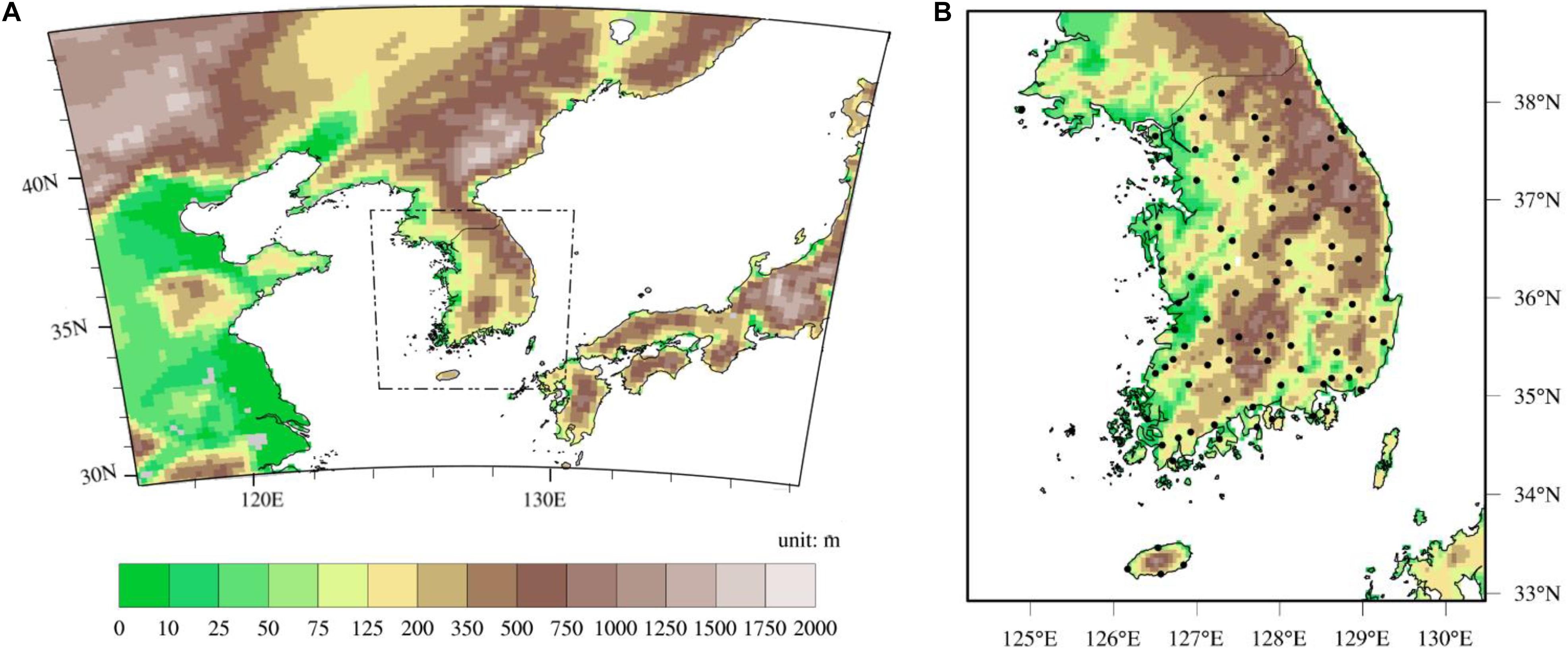
Figure 1. Topography used for the (A) mother domain simulation with 20 km resolution and (B) nested domain simulations with 5 km resolution. The inner dashed black box in (A) marks the domain used for nested run. The 90 black dots in (B) denote the location of in-situ observational stations.

The physical parameterizations of the modeling system follow the optimal setting that Qiu et al. (2020) found through various sensitivity experiments. They can be briefed as: the WSM3 microphysics scheme (Hong et al., 2004), the RRTMG longwave and shortwave radiation scheme (Iacono et al., 2008), the Revised MM5 surface layer scheme (Jiménez et al., 2012), the Noah Land Surface Model scheme (Chen and Dudhia, 2001), the Yonsei University planetary boundary layer scheme (Hong et al., 2006), and the Kain–Fritsch convection scheme (Kain et al., 2008) with trigger function (Ma and Tan, 2009). The same configuration is applied for the mother and the nested domain. Note that we decide to use convection scheme for nested domain after testing the performance of convection permitting simulation.

The initial and boundary conditions are obtained from the CFSv2 operational forecasts at 0.5° × 0.5° resolution at 6-h intervals (Saha et al., 2014). The simulations span from 2011 to 2020 (10-year), for the summer season (June, July, and August). The CFSv2 releases ensemble members with different initialization times of the 0000, 0600, 1200, and 1800 UTC cycles for each day, which allows us to obtain many ensemble members on a regular basis. As a pilot study here, only two ensemble members initialized at 0600 and 1800 UTC are downscaled for each month, and individual runs assign a three-day spin-up period that is excluded from analysis. As a case in point, CFSv2 forecast fields initialized at 0600 and 18:00 UTC, 28 May 2011 are downscaled until 0000, 1 Jun 2011, and the ensemble results encompassing the entire month of June are analyzed to evaluate the prediction performance for June 2011. We are not unaware of the importance of probabilistic prediction from many ensemble members, and thus implying that two members should not be sufficient. While this study aims at evaluating the basic performance of CFSv2 and WRF nested simulations with an emphasis on the added value of dynamical downscaling, further improvement based on the time-lagged ensemble approach using rigorous statistical method should be the focus of future researches.

The model is run twice for the same time period of each simulation, once without SN and once with SN. The effect of SN can be controlled by modulating nudged variables, nudging coefficients, and wave numbers. In this study, horizontal winds, temperature, and geopotential height are nudged with the nudging coefficients of 0.0003 s⁻¹, whereas nudging wave numbers in both zonal and meridional directions are set to be 3. Consistent with the time interval of the input CFSv2 data, nudging is conducted every 6 h, In addition, the spectral nudging is applied to solely the mother domain, and no nudging is conducted within the planetary boundary layer (PBL) to maximize the freedom of mesoscale circulation within the PBL (Liu et al., 2012; Otte et al., 2012; Tang et al., 2017).

For the validation of the downscaled results and CFSv2, we use the 90 in-situ observational data maintained by the Korea Meteorological Administration during the same period of simulation (2011–2020) over South Korea (Figure 1B). The Korean territory is covered by a dense observational network, however, the majority of the stations are situated below 400 m with two exceptional places (Daegwallyeong, 772.4 m; Taebaek, 714.45 m). The lack of observations at a higher elevation may be an impediment in assessing the superiority of high-resolution simulation particularly expected from higher mountainous areas.

Results

Added Value for Mean Temperature and Maximum Temperature

We begin our analysis with the climatological pattern of Tmean and Tmax, which are agriculture-relevant variables used for the calculation of agro-meteorological indices. Figure 2 depicts the spatial distributions of the 10-year (2011–2020) averaged Tmean and Tmax for JJA, and their bias patterns (simulation minus observation) are also presented in Figure 3. For comparison purposes, in-situ observational data and the original CFSv2 data are interpolated into the 5 km grid that is same as the WRF nested domain, using the distance-weighted average remapping function in CDO programming. The observational distribution shows that the Tmean roughly follows the topographical pattern. More specifically, there are two low-lying basins, the Yeongsan River basin (southwest) and the Nakdong River basin (southeast), with relatively high temperature while a distinctly colder temperature is found on the Taebaek Mountains along the northeast. For CFSv2, it is too coarse to be able to capture such regional details in response to topographical fluctuation. CFSv2 can only simulate a very rough spatial division of temperature, such as higher temperature in the southwestern coastal region and lower temperature in the northern part of South Korea. In contrast, the downscaling with WRF, benefitting from its higher-resolution surface boundary conditions, helps to reveal topographically modulated patterns. Besides the spatial details, the downscaled result shows the superior performance to its driving global model in terms of the quantitative measure. WRF result retains the negative bias seen in CFSv2 as compared to observed one, but its severity tends to be reduced. With regard to the Tmax, the improvement derived from dynamical downscaling becomes far more drastic. Tmax from CFSv2 do not differ much with Tmean, thus showing a substantial amount of negative bias (Figure 3D). This is because CFSv2 produces a very small amplitude of diurnal variation of temperature (not shown). Therefore, CFSv2’s performance to capture the peak values (e.g., maximum, minimum) is very limited, although it seems to reveal the error within an acceptable range in terms of mean value. On the other hand, the downscaled Tmax is much closer to the observed pattern both quantitatively and qualitatively, despite the presence of some negative bias. A larger discrepancy between observed and downscaled Tmax is found along the high mountainous region because WRF simulates far lower values than observation (Figures 3C,F).

FIGURE 2

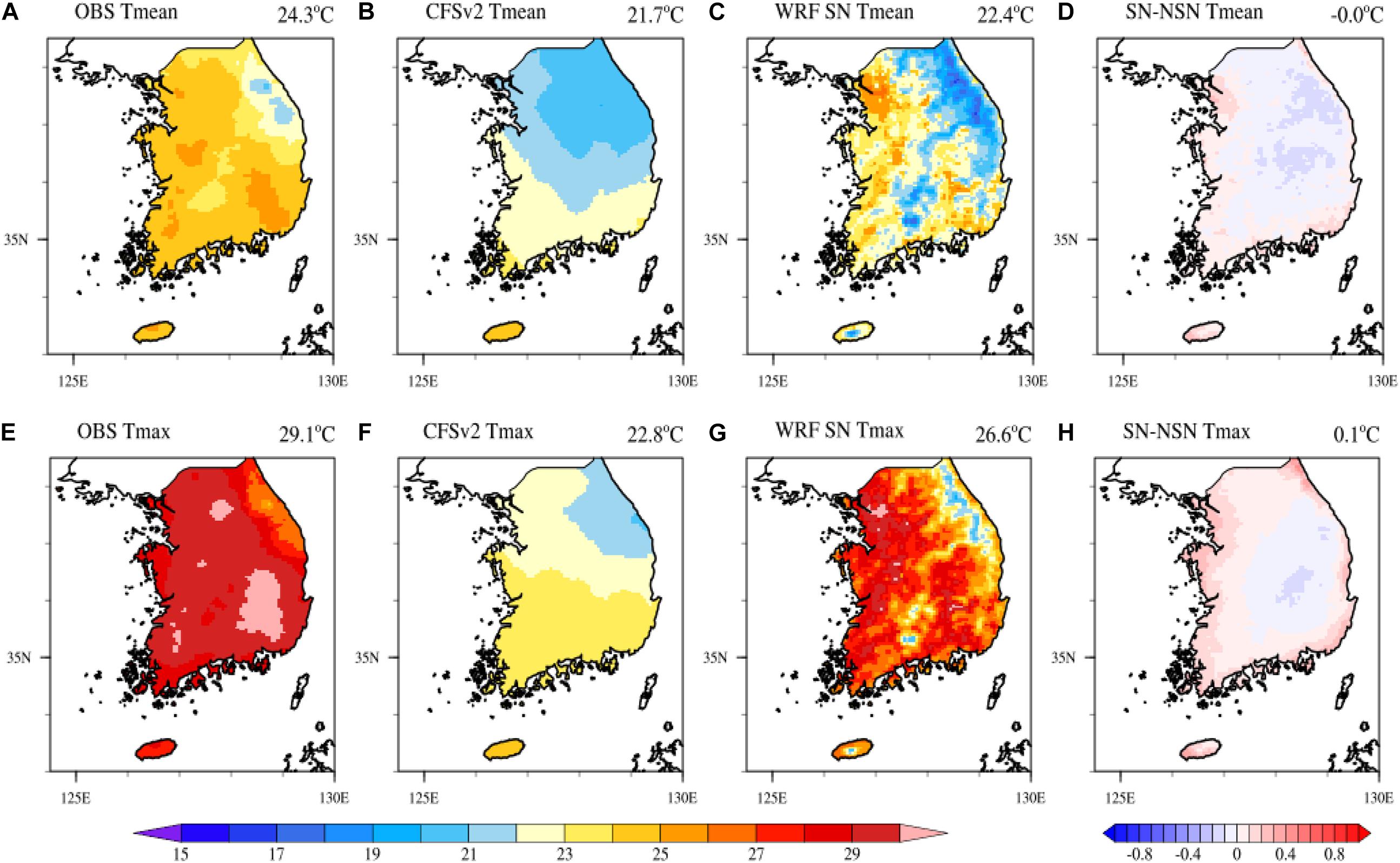
Figure 2. Spatial distribution of JJA 10-year averaged (2011–2022) Tmean (top row) and Tmax (bottom row) from (A,E) observational station data (OBS); (B,F) CFSv2; and (C,G) WRF 5 km simulation with spectral nudging (WRF SN) over South Korea. (D,H) are the difference between WRF simulations with and without SN (SN-NSN). The value at the top right of individual figure panels indicates the average temperature over South Korea.

FIGURE 3

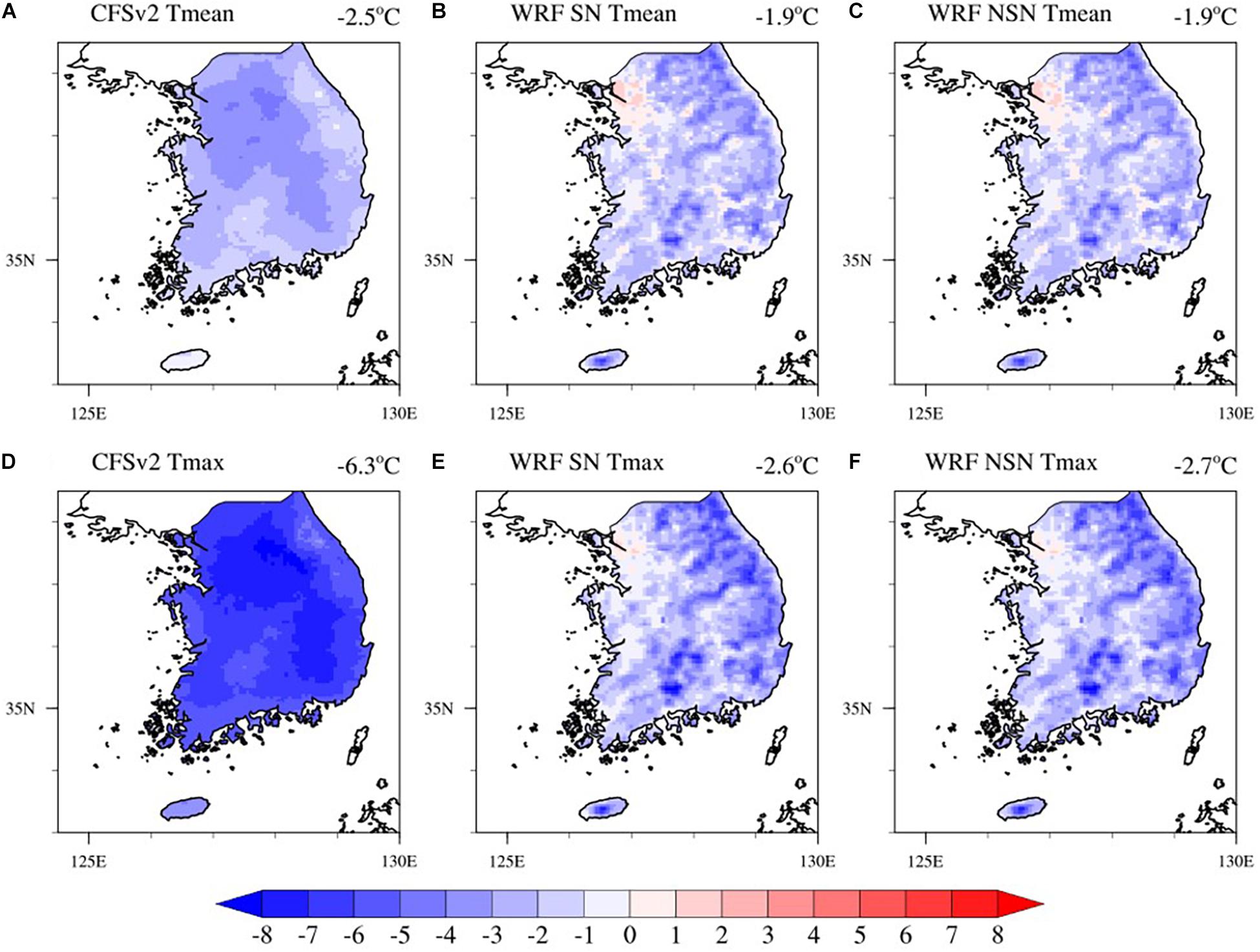
Figure 3. Spatial distribution of bias of Tmean (top row) and Tmax (bottom row) from (A,D) CFSv2 and WRF 5 km simulations (B,E) with spectral nudging (WRF SN) and (C,F) without spectral nudging (WRF NSN) over South Korea.

However, it is partly attributed to the scarcity of in-situ stations at higher elevations. Notably, a sharp temperature gradient along the northeastern coastlines is brought by the elevation slope between the mountain and the coast. Such a gradient is even obscured on the interpolated observation map due to the limited number and uneven distribution of observation stations, whereas the downscaled result clearly shows a narrow “warm band” along the coastlines. The difference between downscaled results with and without SN reveals that in terms of climatological mean, the effect of SN in our target domain seems to be marginal. The simulation with SN tends to slightly increase the temperature along the coastline as compared to the one without SN (hereafter referred to as NSN), but opposite over the large inland region. The magnitude of such differences is very smaller than the model bias, and thus it is hard to discern the bias patterns between SN and NSN (Figures 3B,C/Figures 3E,F). Although we first compare the simulations with an interpolated observation in Figures 2, 3 to clearly compare the spatial distribution of temperatures that are strongly tied to physiographical features (e.g., topography), we also perform station-based point-wise analysis afterwards. For this purpose, the nearest grid to the station is selected from WRF 5 km simulations. Since the model resolution (i.e., 5 km) is higher than the mean distance of stations, no station values are from the same grid. For comparison purpose, CFSv2 is first interpolated into WRF 5 km grid and the nearest grid is then selected as well.

In order to evaluate the performance of simulations in a more quantitative manner, we compare the Taylor diagrams of Tmean and Tmax in the months of June, July, and August (Figure 4). The Taylor diagram is convenient to quantify the multiple metrics in terms of the pattern correlation, the centered root-mean-square (RMS) error and the standard deviation in a single plot (Taylor, 2001). The centered RMS error and standard deviation are normalized by the standard deviation of observation. With regard to the pattern correlation represented by the azimuthal position, it is obvious that the downscaled WRF simulations show a substantial improvement in both Tmean and Tmax. In particular, the difference of correlation coefficient between CFSv2 and WRF becomes much higher in Tmax than in Tmean, which agrees well with the spatial distribution observed in Figure 2. The correlation coefficients of Tmax are increased by approximately more than 2-fold in WRF than in CFSv2 for all 3 months. The deficiency of CFSv2 is not limited to only spatial correction, but the RMS error is also greater than the downscaling results. In terms of the standard deviation, WRF and CFSv2 exhibit a starkly contrasting behavior. While the standard deviation of CFSv2 holds lower than 1 (except for Tmean in Aug), the downscaled results exhibit a larger amplitude of spatial variability compared to the observed one. This could be attributed to the very fine-resolution of WRF simulations, which are capable of resolving the sharp gradients of temperature change within a short distance (Qiu et al., 2020). The CFSv2 and its downscaling results also behave differently in terms of the fluctuation of performance across months. For CFSv2, the relative skills with respect to the months and between Tmean and Tmax seem to be inconsistent, being particularly problematic in June with the large failure to capture spatial pattern and variability amplitude. On the other hand, the downscaled results tend to keep the performance stable. The numbers corresponding to the months are closely positioned, relative to those from CFSv2. By comparing WRF simulations with and without SN, it is again revealed that the effect of SN may not be relevant. The NSN simulation seemingly does exhibit slightly better statistics, but the difference of their positions between SN and NSN is marginal. For the sake of simplicity, we only present the NSN result in the rest of section “Added Value for Mean Temperature and Maximum Temperature.”

FIGURE 4

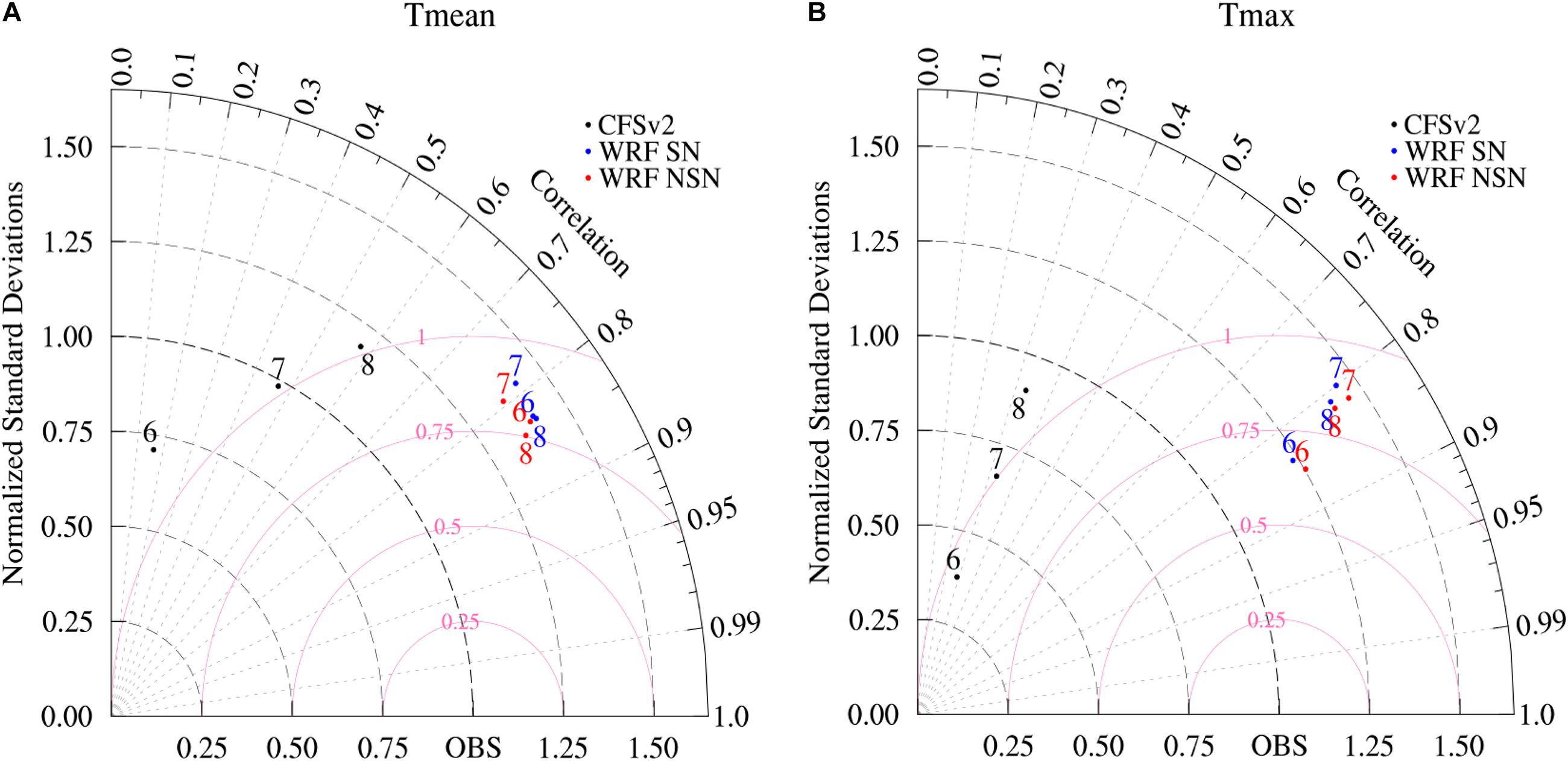
Figure 4. Taylor diagram of monthly mean (A) Tmean and (B) Tmax calculated from the three individual simulations against in-site observations at 90 stations. The semicircles marked with the pink line indicate the centered of root-mean-square (RMS) error. The numbers of 6, 7, and 8 correspond to the months of June, July, and August, respectively.

The 10-year length simulation allows further assessment of the skill to capture the interannual variability of summer temperature. Figure 5A illustrates the Tmean and Tmax anomalies derived from observation, CFSv2 and WRF downscaled result. The anomaly of Tmean (Tmax) is calculated as each year’s JJA deviation from 10-year climatological JJA Tmean (Tmax) averaged over 90 stations during the 10-year period. By comparing with the observation, CFSv2 captures at least the same sign of yearly variability because the systematic cold bias shown in Figures 2, 3 can be partly eliminated while subtracting the mean climatology. However, CFSv2 may not have the ability to simulate particularly hot (e.g., 2018) and cold (e.g., 2014) years. This problematic behavior exacerbates in Tmax, thus implying the limited performance in simulating extreme case. The downscaled result tends to maintain much of the behavior seen in CFSv2. However, the added value of dynamical downscaling is more apparent when evaluated with respect to each station, rather than taking the spatially average values. Figures 5B,C depict the box plot of Tmean and Tmax anomalies at 90 stations, respectively. The observational pattern shows a large variability across stations. For example, the stations with negative or positive anomalies co-exist for most of years. Such a behavior is more pronounced in Tmax than in Tmean. On the contrary, a very small range of variability across stations is the most relevant feature of CFSv2. This simply indicates that CFSv2 fails to capture the regionally distinct temperature patterns. The ranges of the interannual variability of the downscaled Tmean, though still narrow as compared to the observation, are much greater than the CFSv2, thereby proving the potential benefits of dynamic downscaling.

FIGURE 5

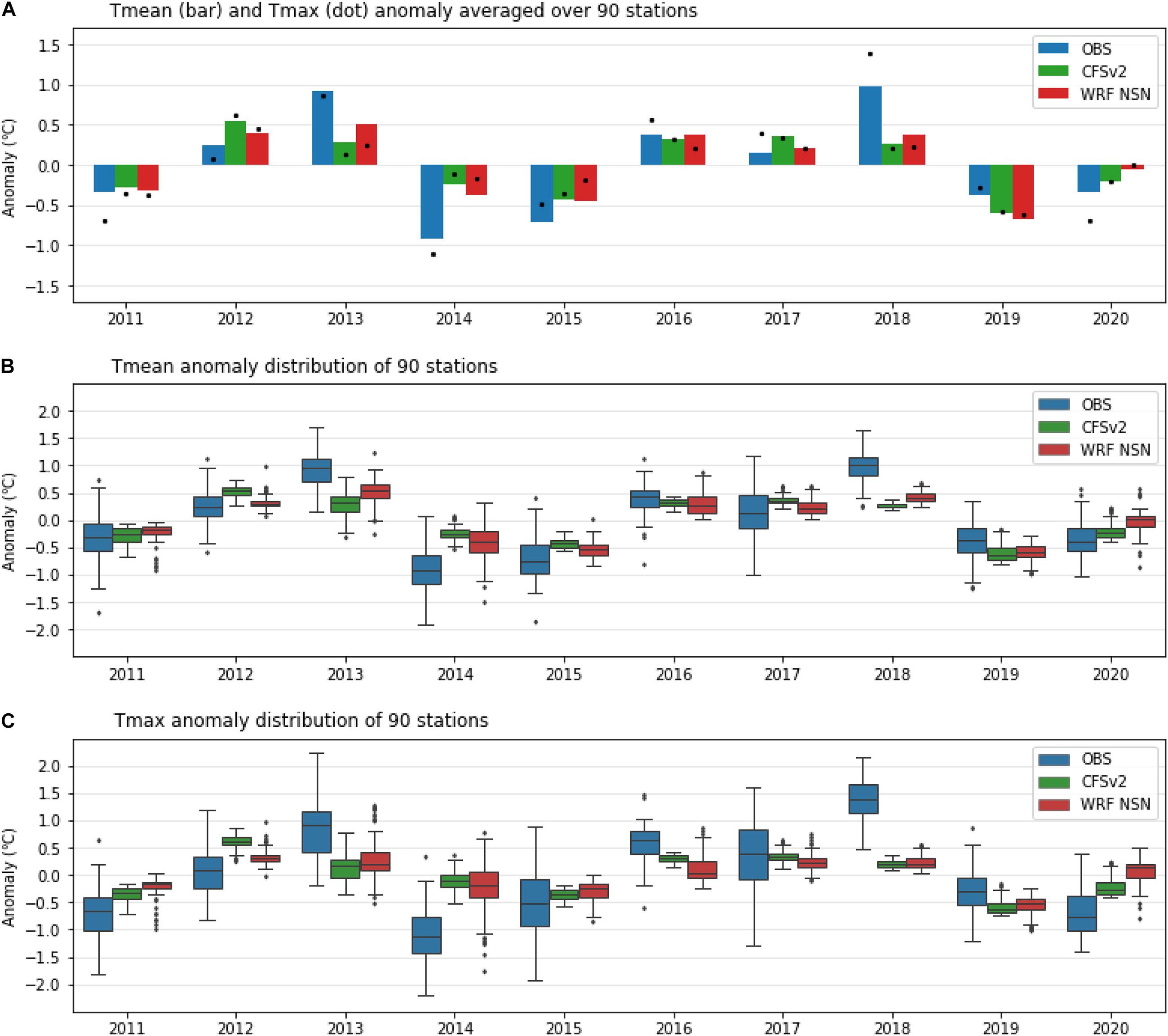
Figure 5. (A) Interannual variation of JJA Tmean (bar) and Tmax (dot) anomalies that are calculated based on 90 stations averaged Tmean and Tmax. (B,C) are boxplots of JJA Tmean and Tmax deviations of that year from the 10-year climatology (i.e., anomaly) at 90 stations.

Figure 6 presents the scatterplot of the Pearson correlation coefficient (CC) among all the pairwise combinations of the 90 stations (4,005 pairs in total), which measures the temporal linear dependency of temperatures vs. their actual distance in space. A higher CC value indicates a higher similarity between paired stations. Usually, the closer the distance between paired stations, the greater the correlation between them. The observation pattern well demonstrates that the spatial dependence of both Tmean and Tmax decreases gradually when the distance increases. Unlike Tmean, Tmax shows a more obvious declining trend beginning from a shorter distance between the paired data. However, CFSv2 provides a much smoother CC gradient along the distance. It retains CCs higher than 0.8 for Tmean and higher than 0.7 for Tmax. Such high correlations are in accordance with its failure to capture spatial details of temperature pattern as mentioned above. In contrast, the downscaled results are in good agreement with the observational pattern, capturing the similar gradient of the decreasing CC along the distance. They yield the decreasing CC even for the short distance range, indicating the potential of dynamical downscaling in simulating the localized temperature patterns.

FIGURE 6

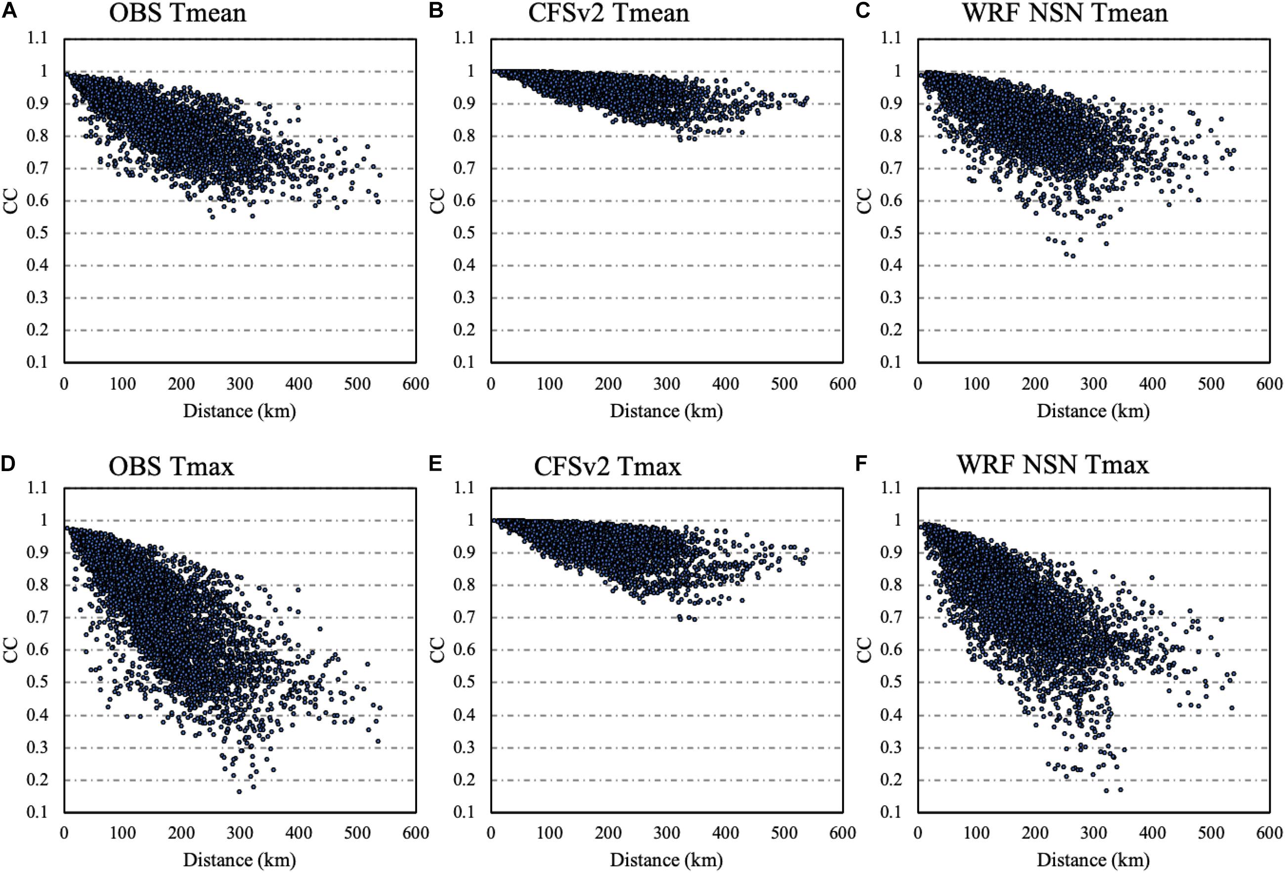
Figure 6. Scatterplot of the correlation coefficients (CC) for Tmean (top row) and Tmax (bottom row) vs. their inter-station distances (90 stations) derived from (A,D) OBS; (B,E) CFSv2; and (C,F) WRF NSN.

To understand the different performance of Tmean and Tmax seen in CFSv2 and the WRF downscaled result, we investigate the relationship between elevation and bias. Figure 7 presents a scatter plot of the difference in elevation between the model grid and the actual station against Tmean and Tmax biases. As the degree of scattering is smaller, the model is in better agreement with the observed value. Generally, the magnitude of temperature bias has been seen to be correlated to the difference of elevation in the model from actual height. Since CFSv2 prescribes higher elevations in the majority of stations as compared to actual values (90-station-average difference: 61.4 m), it tends to aggravate the cold bias. Although the cold bias is not linearly scaled with the elevation difference, the larger cold bias is evidently found mainly where the model’s elevation is higher. The resolution of CFSv2 may not be able to accurately resolve the low-lying area, which is why it does not reveal the two basins at a higher temperature in Figure 2B. As for Tmax, CFSv2’s cold bias becomes far greater than Tmean, holding the negative relationship between elevation and temperature biases. It is noteworthy that many more observational stations are located in the low elevation regions than their high counterparts. Therefore, the cold biases arising from an overestimation of elevation seems to be more dominant in Figure 7. However, the coarse resolution of CFSv2 also underestimates the elevation of high mountains that causes the missing of “cold peak” in the Tmean spatial pattern. On the other hand, the temperature bias in WRF is much smaller, which can be explained by the more realistic elevation (90-station-average elevation difference: 42.7 m).

FIGURE 7

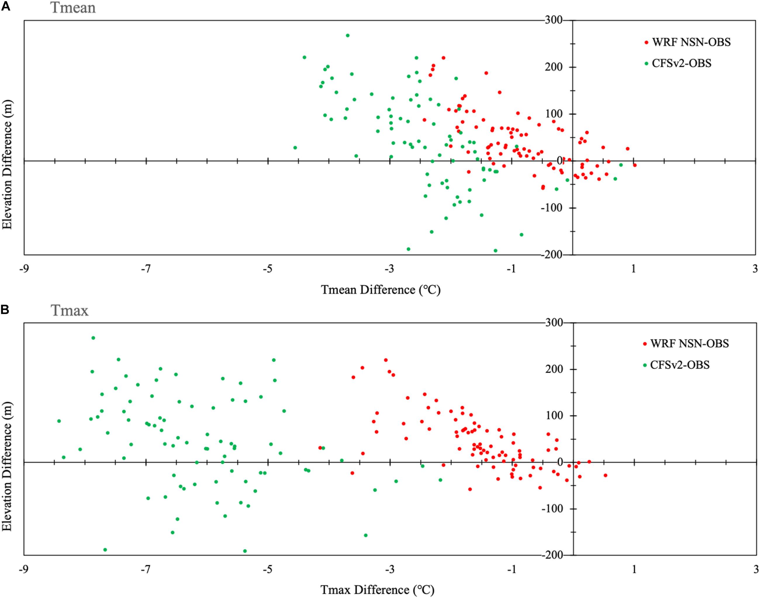
Figure 7. Scatterplot of the elevation difference between station and nearest model grid against the bias of JJA 10-year averaged (A) Tmean and (B) Tmax at 90 stations. CFSv2 and WRF NSN results are displayed with green and red dots, respectively.

Evaluation of Agro-Meteorological Indices

In this section, we evaluate the performances of the downscaled result in simulating agro-meteorological indices. As shown in Figures 2, 3, CFSv2 exhibits a severe cold bias over the entire domain. It is observed that Tmax from CFSv2 never reaches 30°C at any of the stations, which prevents the calculation of PHS and EDD. Therefore, we do not present the results from CFSv2 and focus on the evaluation of WRF simulations with and without SN in this section. Figure 8 illustrates the total sum of the PHS (number of days with Tmax exceeding 30°C) during 10-year (2011–2020) derived from observed and SN and NSN simulated Tmax. Consistent with the Tmax climatology presented in section “Added Value for Mean Temperature and Maximum Temperature,” the model tends to underestimate PHS. However, considering the severe cold bias seen in CFSv2, this result unambiguously proves the potential of dynamical downscaling for making improvement in the simulations of heat extremes, particularly in the low-lying basin region. Contrary to the fact that the effect of SN seems to be concealed in the climatological mean pattern, the difference between SN and NSN is better detected in the analysis of extremes based on daily data. In general, SN appears to be a little more helpful in alleviating the underestimation, except for several stations located near the eastern coast.

FIGURE 8

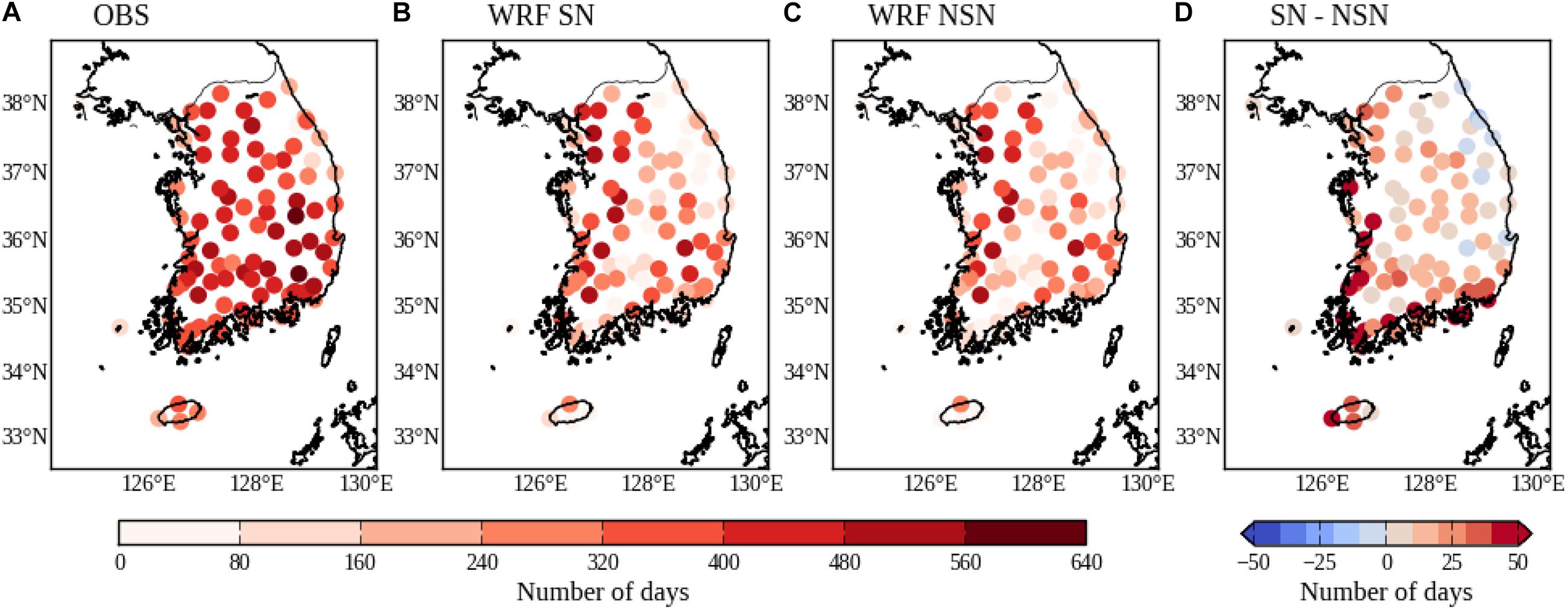
Figure 8. Spatial distribution of the JJA 10-year (2011–2020) sum of the PHS index (number of days with Tmax exceeding 30°C) at 90 stations derived from the (A) observations, the (B) SN and (C) NSN simulations, and the (D) difference between SN and NSN (SN–NSN).

As another agro-meteorological index, we investigate the performance of how the model with SN and NSN can simulate the characteristics of EDD. The EDD is calculated with respect to 90 stations using hourly temperature data as follows.

$$\text{EDD}=\sum _{\text{t}=1}^{\text{N}}\left({\text{T}}_{\text{t}}-30\right)/24,\mathrm{if}{\mathrm{T}}_{\text{t}}>30{}^{°}\mathrm{C}$$

(where t varies from 1 to 2,208 (24-h × 92 d), covering from 1 June to 31 August).

After first calculating the EDD for individual years, the 10-year average is presented in Figure 9. Basically, the behavior of EDD is quite in line with PHS, with respect to the similarity and difference between observation and simulation. Compared to observation, the underestimation consistently appears in the WRF model results. However, dynamical downscaling is able to draw prominent results in some stations. For example, the most intense heat observed in Daegu is well reproduced in both NSN and SN simulations.

FIGURE 9

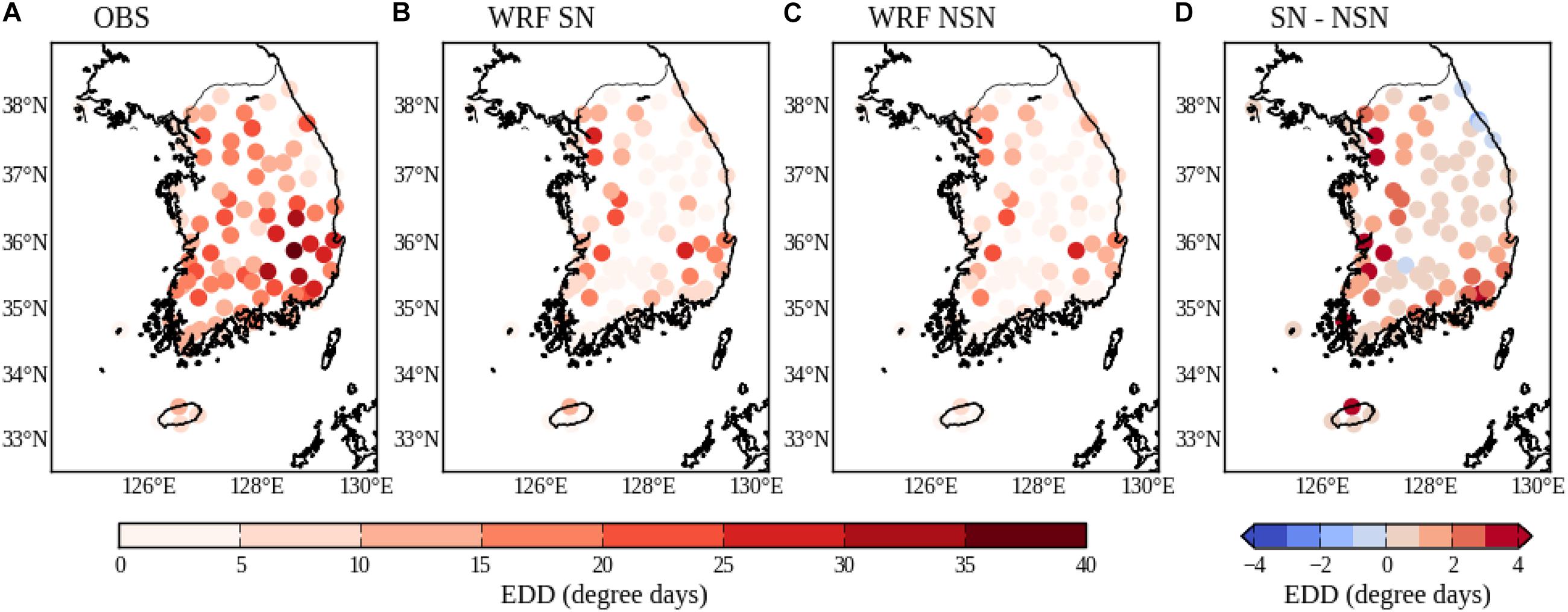
Figure 9. Spatial distribution of the JJA 10-year (2011–2020) averaged EDD index at 90 stations derived from the (A) observations, the (B) SN and (C) NSN simulations, and the (D) difference between SN and NSN (SN–NSN).

In addition to total accumulated EDD, its evolutionary pattern also denotes critical information for agriculture application. Therefore, we investigate the temporal evolution of EDD through three months (June-July-August) with regard to individual years. Figure 10 displays the evolutionary pattern of EDD at three stations, namely, Daejeon, Daegu, and Mokpo, located in the northwestern, southeastern, and southwestern part of the country, respectively. For the observational pattern, EDD shows the pronounced yearly variation and regional disparity. EDD patterns in anomalously hot years (e.g., 2018) are totally different from anomalously cold years (e.g., 2014). For example, in Daejeon, the accumulated EDD at the end of August is over seven times larger in 2018 than in 2014. Similarly, the regional pattern is also quite diverse. While EDD marks the second highest value (around 60 degree days) in Daegu in 2013, its accumulated value is less than 20 degree days at the end of August in both Daejeon and Mokpo. Again, such a regionally distinct pattern highlights the necessity of fine-scale meteorological data. Among a large difference across years and stations, a common feature is seen in most stations. The EDD is primarily accumulated from mid-July to mid-August, which determines the total amount of EDD for individual years. More specifically, the increment of EDD seems to be small until the mid-July, and then its increasing rate sharply rises until mid-August before tending to hold a somewhat flat curve. In general, the anomalous warm years show the steep gradient of EDD increment. The simulations show a reasonable performance in capturing such an evolutionary pattern of EDD varying across the months regarding most of normal years (e.g., relatively smaller anomaly seen in Figure 5A). However, as addressed in the interannual variability, the downscaled results also reveal limited accuracy in capturing extreme years like 2018. This failure is mainly attributed to the predictability skill of CFSv2 because the large-scale synoptic conditions to determine anomalously warm or cold summers are inherited by the WRF simulation. In addition, the models’ ability to capture different regional pattern merits attention. Similar to the observational pattern, the WRF simulations effectively capture high EDD at Daegu and lower EDD at Mokpo. In comparison to NSN, SN tends to yield a slightly higher EDD at the end of August. Such a behavior leads to some improvement in Daejeon and Mokpo, but the effect of SN is marginal in Daegu. Despite some deficiencies, this analysis reflects the potential of downscaled results for predicting heat-related agro-meteorological indices, which would otherwise be unfeasible with the direct usage of CFSv2 global prediction.

FIGURE 10

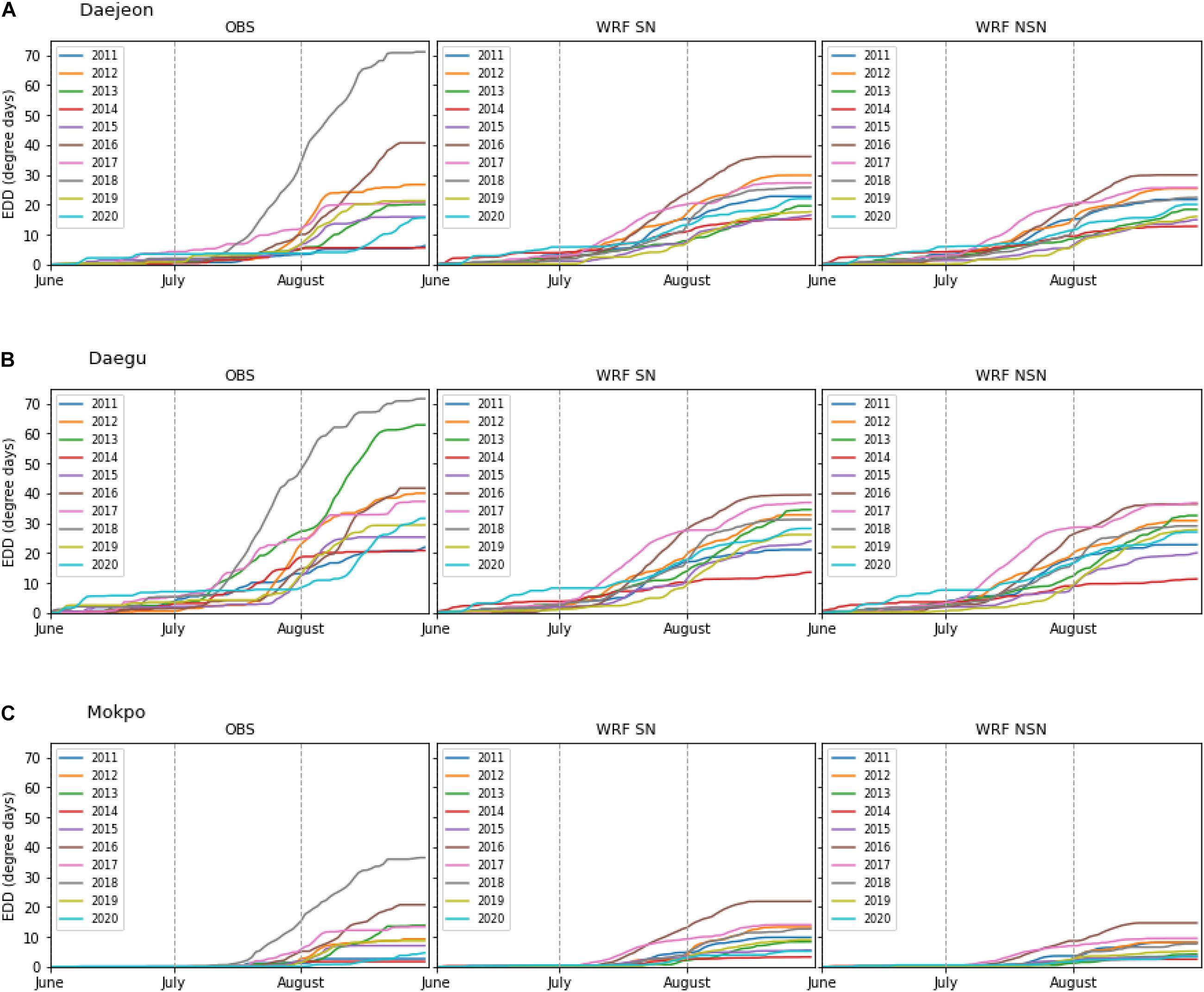
Figure 10. The time evolution of EDD index from June to August for individual years at (A) Daejeon, (B) Daegu, and (C) Mokpo stations derived from the observations, SN and NSN simulations.

Although it is important to prepare for the damage caused by the exposure of extreme Tmax, the negative effect caused by the increase of Tmean is also highly expected amid global warming. In this regard, we calculate an index based on Tmean. The accumulated heat stress (AHS) that is critical for the reproductive growth of rice is defined as follows, under consideration of the reproductive growth stage for mid-late maturing rice cultivars (Shin et al., 2019) and 24°C of Tmean where the rice spikelet fertility starts to decrease (Loc Thuy et al., 2020).

$$\text{AHS}=\sum _{\text{t}=1}^{\text{N}}\left({\text{Tmean}}_{\text{t}}-24\right),\mathrm{if}{\mathrm{Tmean}}_{\text{t}}>24{}^{°}\mathrm{C}$$

(where, t varies from 11 July to 15 August).

Figure 11 presents the interannual variation of AHS averaged over 90 stations. Consistent with the underestimation of Tmean presented in Figures 2, 3 AHS derived from simulations is systematically lower than observed one. In addition, the model-based AHS is unable to discern the spiked feature of an extremely hot year like 2018. However, WRF simulations show the potential to capture the general range of AHS in normal years. Furthermore, the spatial distribution of 10-year climatological AHS shows a good agreement between simulation and observation, which is quite similar to that of the PHS index (not shown). As clearly indicated by observed AHS, relevant AHS is already emerging under the current climate condition and is likely to be more pervasive in the future, suggesting the necessity of cultivars with improved heat stress tolerance (Loc Thuy et al., 2020).

FIGURE 11

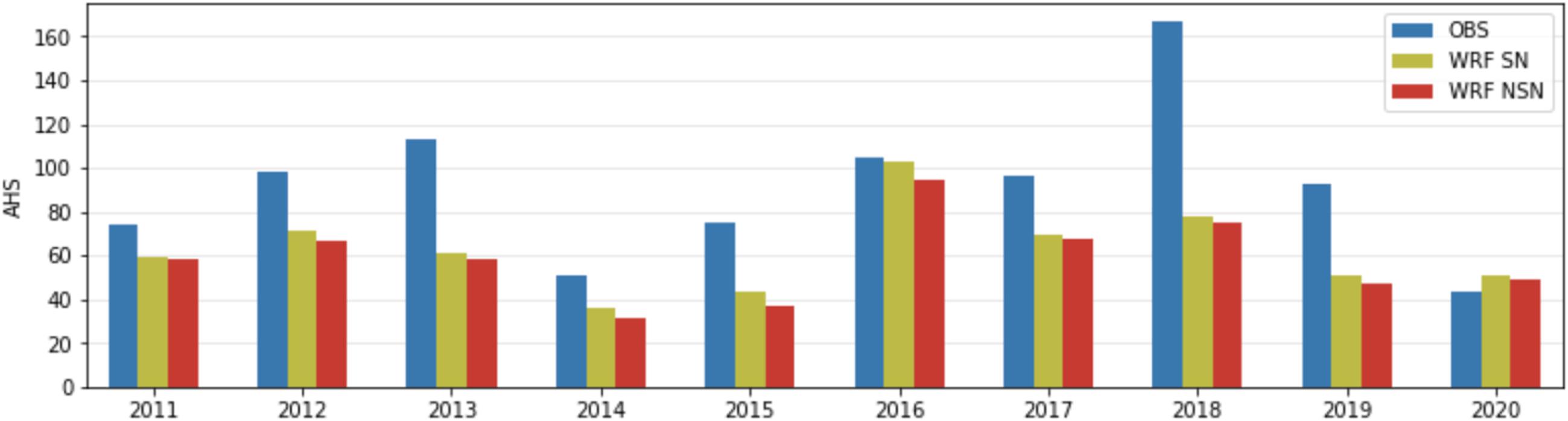
Figure 11. The interannual variation of AHS averaged over 90 stations derived from the observations, SN and NSN simulations.

Summary and Discussion

Improving the prediction accuracy of meteorological condition at subseasonal time-scale is a complex and multifaceted problem (Min et al., 2020). In this study, our aim is confined to demonstrating the added value that can be derived from the dynamical downscaling through comparison with driving global forecast data. For this purpose, our evaluation is performed in a “deterministic” way after the arithmetic ensemble mean of two members with different initial times (06UTC and 18UTC). We are aware of the insufficiency of two members as well as the importance of probabilistic prediction using many ensemble members, especially for the long lead time. For future studies, many more ensemble members will be generated by applying the time-lagged ensemble approach and we will develop the probabilistic forecast system using higher order statistical technique (e.g., Bayesian hierarchical model, Wang et al., 2016).

The CFSv2 global prediction for summer of the past 10-year (2011–2020) shows the ability to at least capture the area-averaged temperature anomaly (e.g., hot summer or cold summer against climatological mean). However, CFSv2 has a severe cold bias over the entire Korean territory, and its error increases significantly in Tmax, thus posing a major challenge for predicting extremes. Additionally, CFSv2’s coarse resolution could not effectively represent the spatial variability associated with topographical modulation. On the other hand, dynamical downscaling using the WRF nested system leads to a significant improvement in both quantitative and qualitative aspects. Since the predictability to capture extremely hot summers like the one in 2018 stems from skill related to global prediction, the downscaled result also retains quite a limited accuracy in predicting extreme years. However, the downscaled results show the considerable reduction of cold bias and a drastic improvement in spatial variability. The added value of downscaling appears even greater in Tmax than in Tmean. This is particularly beneficial when it comes to calculating agro-meteorological indices pertaining to heat stress. By comparing SN with NSN, the positive effect of SN is not clearly evidenced from our simulations. Although the cold bias in agro-meteorological indices can be reduced a bit when SN is employed, the improvement seems to be marginal. This result may be supported by Schaaf et al. (2017) that showed little effect of SN when the model domain is relatively small.

Since this study is the first attempt to perform dynamical downscale of CFSv2 focusing on the Korean peninsula, it is not allowed to benchmark our results against other literatures. However, we found a study that demonstrated the performance of dynamical downscaling of CFSv2 in Vietnam using the RegCM4 (Phan-Van et al., 2014). Their downscaling results show the severe cold temperature exceeding −5°C at a month lead time. The magnitude of this bias is larger than our simulation. However, the quantitative comparison is not meaningful because the experimental design is not similar to each other in terms of the target region (Korea vs. Vietnam), resolution (5 vs. 36 km), and RCM (WRF vs. RegCM4). Nevertheless, it would be reasonable to infer that the temperature biases of WRF simulations presented in this study are in the acceptable range.

While the downscaled results show an encouraging performance in simulating the temperature climatology and temperature-based agro-meteorological indices over Korea with added values beyond driving CFSv2, it does not necessarily guarantee that other variables, such as precipitation and radiation, which are critical to crop yield, are also simulated in a reasonable manner. In particular, the precipitation simulations often reveals substantial errors in many regions worldwide (e.g., Wang et al., 2015; Guo et al., 2017). The positive effect of higher resolution through dynamical downscaling may not be straightforward to precipitation performance (Im and Eltahir, 2018) in comparison to temperature. Moreover, summer precipitation over Korea shows a large variability, thereby making its forecast much more challenging (Nguyen-Xuan et al., 2020). Further work focusing on the performance of precipitation and precipitation-based agro-meteorological indices will be conducted for the subsequent paper.

While being aware of a critical need and the potential benefit of meteorological information, their utilization remains constricted for actual decision processes and activities to enhance agriculture production. The main impediment should be the scale mismatch as well as the absence of high quality and long-term forecast data. The Korea Meteorological Administration has publicly released forecast data up to 10-days. However, such a lead time may not be sufficient enough to allow farmers to schedule the variety field activities. Finer-scale, longer-term meteorological forecast data needs keen attention. In particular, since extreme hot temperatures have emerged as one of the disaster-related threats in Korea due to accelerated global warming (Im et al., 2017, 2019), the agricultural sector is very likely to be adversely affected if preparations are not made in a timely manner (e.g., Shin Y.-H. et al., 2017; Jo et al., 2020). From the perspective of climate change adaptation, the value of meteorological forecast data will continue to enhance. Indeed, the fine-scale long-term forecasting meteorological datasets are versatile enough to directly link to the agriculture impact assessments. More specifically, temperature and rainfall data are used as the input for statistical empirical models (e.g., multiple regression, support vector machine) to predict reliable yield estimates (e.g., Joshi et al., 2020). The process-based crop models (e.g., Decision Support System for Agrotechnology Transfer, DSSAT) also require fine-scale meteorological data as the most important input because weather conditions can regulate the growth and yield of crops. In this regard, further improvement in the accuracy of downscaled results by incorporating the probabilistic ensemble technique and post-processing method, such as bias-correction will be transferable to improving actual agriculture modeling.

Data Availability Statement

The datasets presented in this study can be found in online repositories. The names of the repository/repositories and accession number(s) can be found below: the CFSv2 data is openly available at the following URL: https://www.ncdc.noaa.gov/data-access/model-data/model-datasets/climate-forecast-system-version2-cfsv2. The downscaled data and ncl and python scripts used for the analysis are available from the corresponding author upon reasonable request.

Author Contributions

E-SI and JH conceived this study. SH and LQ performed the simulations and analyzed the output. E-SI wrote the majority of manuscript with inputs from SH, LQ, JH, SJ, and K-MS. All authors discussed the results.

Funding

This study was carried out with the support of “Research Program for Agricultural Science & Technology Development (Project No. PJ014882),” National Institute of Agricultural Sciences, Rural Development Administration, South Korea.

Conflict of Interest

The authors declare that the research was conducted in the absence of any commercial or financial relationships that could be construed as a potential conflict of interest.

Acknowledgments

We thank the two reviewers for their constructive comments. The details about WRF model can be found in user’s manual (https://www2.mmm.ucar.edu/wrf/users/docs/user_guide_v4/v4.2/WRFUsersGuide_v42.pdf).

References

Cha, D.-H., Jin, C.-S., Lee, D.-K., and Kuo, Y.-H. (2011). Impact of intermittent spectral nudging on regional climate simulation using Weather Research and Forecasting model. J. Geophys. Res. 116:D10103. doi: 10.1029/2010JD015069

CrossRef Full Text | Google Scholar

Cha, D.-H., and Lee, D.-K. (2009). Reduction of systematic errors in regional climate simulations of the summer monsoon over East Asia and the western North Pacific by applying the spectral nudging technique. J. Geophys. Res. 114:D14108. doi: 10.1029/2008JD011176

CrossRef Full Text | Google Scholar

Chen, F., and Dudhia, J. (2001). Coupling an advanced land surface – hydrology model with the Penn State – NCAR MM5 modeling system. Part I: model implementation and sensitivity. Mon. Weather Rev. 129, 569–585.

Google Scholar

Gao, X., Xu, Y., Zhao, Z., Pal, J. S., and Giorgi, F. (2006). On the role of resolution and topography in the simulation of East Asia precipitation. Theor. Appl. Climatol. 86, 173–185.

Google Scholar

Guo, J., Huang, G., Wang, X., Li, Y., and Lin, Q. (2017). Investigating future precipitation changes over China through a high-resolution regional climate model ensemble. Earths Future 5, 285–303. doi: 10.1002/2016EF000433

CrossRef Full Text | Google Scholar

Hong, S.-Y., Dudhia, J., and Chen, S.-H. (2004). A revised approach to ice-microphysical processes for the bulk parameterization of cloud and precipitation. Mon. Weather Rev. 132, 103–120.

Google Scholar

Hong, S. Y., Noh, Y., and Dudhia, J. (2006). A new vertical diffusion package with an explicit treatment of entrainment processes. Mon. Weather Rev. 134, 2318–2341. doi: 10.1175/MWR3199.1

CrossRef Full Text | Google Scholar

Iacono, M. J., Delamere, J. S., Mlawer, E. J., Shephard, M. W., Clough, S. A., and Collins, W. D. (2008). Radiative forcing by long-lived greenhouse gases: calculations with the AER radiative transfer models. J. Geophys. Res. 113:D13103. doi: 10.1029/2008JD009944

CrossRef Full Text | Google Scholar

Iizumi, T., Sakuma, H., Yokozawa, M., Luo, J.-J., Challinor, A. J., Brown, M. E., et al. (2013). Prediction of seasonal climate-induced variations in global food production. Nat. Clim. Change 3, 904–908. doi: 10.1038/nclimate1945

CrossRef Full Text | Google Scholar

Im, E.-S., and Ahn, J.-B. (2011). On the elevation dependency of present-day and future climate simulations from a high-resolution regional climate model. J. Meteorol. Soc. Japan 89, 89–100. doi: 10.2151/jmsj.2011-106

PubMed Abstract | CrossRef Full Text | Google Scholar

Im, E.-S., Ahn, J.-B., and Jo, S.-R. (2015). Regional climate projection over South Korea simulated by the HadGEM2-AO and WRF model chain under the RCP emission scenarios. Clim. Res. 63, 249–266. doi: 10.3354/cr01292

CrossRef Full Text | Google Scholar

Im, E.-S., Choi, C.-W., and Ahn, J.-B. (2017). Worsening of heat stress due to global warming in South Korea based on multi-RCM ensemble projections. J. Geophys. Res. Atmos. 122, 11444–11461. doi: 10.1002/2007JD026731

CrossRef Full Text | Google Scholar

Im, E.-S., and Eltahir, E. A. B. (2018). Simulation of the diurnal variation of rainfall over the western Maritime Continent using a regional climate model. Clim. Dyn. 51, 73–88.

Google Scholar

Im, E.-S., Kwon, W.-T., Ahn, J.-B., and Giorgi, F. (2007). Multi-decadal scenario simulation over Korea using a one-way double-nested regional climate model system. Part I: recent climate simulation (1971-2000). Clim. Dyn. 28, 759–780. doi: 10.1007/s10584-009-9691-2

CrossRef Full Text | Google Scholar

Im, E.-S., Nguyen-Xuan, T., Kim, Y.-H., and Ahn, J.-B. (2019). 2018 Summer extreme hot temperatures in South Korea and their intensification under 3^°C global warming scenario. Environ. Res. Lett. 14:094020. doi: 10.1088/1748-9326

CrossRef Full Text | Google Scholar

Im, E.-S., Park, E.-H., Kwon, W.-T., and Giorgi, F. (2006). Present climate simulation over Korea with a regional climate model using a one-way nested system. Theor. Appl. Climatol. 86, 187–200. doi: 10.1007/s00704-005-0215-3

CrossRef Full Text | Google Scholar

Jiménez, P. A., Dudhia, J., González-Rouco, J. F., Navarro, J., Montávez, J. P., and Garcìa-Bustamante, E. (2012). A revised scheme for the WRF surface layer formulation. Mon. Weather Rev. 140, 898–918. doi: 10.1175/MWR-D-11-00056.1

CrossRef Full Text | Google Scholar

Jo, S., Shim, K.-M., Hur, J., Kim, Y.-S., and Ahn, J.-B. (2020). Future changes of agro-climate and heat extremes over S. Korea at 2 and 3 ^°C global warming levels with CORDEX-EA phase 2 projection. Atmosphere 11:1336. doi: 10.3390/atmos11121336

CrossRef Full Text | Google Scholar

Joshi, V. R., Kazula, M. J., Coulter, J. A., Naeve, S. L., and Garcia, A. G. Y. (2020). In-season weather data provide reliable yield estimates of maize and soybean in the US central Corn Belt. Int. J. Biometeorol. 65, 489–502. doi: 10.1007/s00484-020-02039-z

PubMed Abstract | CrossRef Full Text | Google Scholar

Kain, J. S., Weiss, S. J., Bright, D. R., Baldwin, M. E., Levit, J. J., Carbin, G. W., et al. (2008). Some practical considerations regarding horizontal resolution in the first generation of operational convection-allowing NWP. Weather Forecast. 23, 931–952. doi: 10.1175/WAF2007106.1

CrossRef Full Text | Google Scholar

Klopper, E., Vogel, C. H., and Landman, W. A. (2006). Seasonal climate forecasts – potential agricultural-risk management tools? Clim. Change 76, 73–90. doi: 10.1007/s10584-005-9019-9

CrossRef Full Text | Google Scholar

Lee, M.-H., Im, E.-S., and Bae, D.-H. (2019a). Impact of the spatial variability of daily precipitation on hydrological projections: a comparison of GCM- and RCM-driven cases in the Han River basin, Korea. Hydrol. Process 33, 2240–2257.

Google Scholar

Lee, M.-H., Lu, M., Im, E.-S., and Bae, D.-H. (2019b). Added value of dynamical downscaling for hydrological projections in the Chungju Basin, Korea. Int. J. Climatol. 39, 516–531. doi: 10.1002/joc.5825

CrossRef Full Text | Google Scholar

Liu, P., Tsimpidi, A. P., Hu, Y., Stone, B., Russell, A. G., and Nenes, A. (2012). Differences between downscaling with spectral and grid nudging using WRF. Atmos. Chem. Phys. 12, 3601–3610. doi: 10.5194/acp-12-3601-2012

CrossRef Full Text | Google Scholar

Liu, S., Wang, J. X. L., Liang, X.-Z., and Morris, V. (2016). A hybrid approach to improving the skills of seasonal climate outlook at the regional scale. Clim. Dyn. 46, 483–494. doi: 10.1007/s00382-015-2594-1

CrossRef Full Text | Google Scholar

Lobell, D. B., Hammer, G. L., Mclean, G., Messina, C. D., Roberts, M. J., and Schlenker, W. (2013). The critical role of extreme heat for maize production in the United States. Nat. Clim. Change 3, 497–501. doi: 10.1038/nclimate1832

CrossRef Full Text | Google Scholar

Loc Thuy, T., Lee, C.-K., Jeong, J.-H., Lee, H.-S., Yang, S.-Y., Im, Y.-H., et al. (2020). Impact of heat stress on pollen fertility rate at the flowering stage in korean rice (Oryza sativa L.) cultivars. Korean J. Crop Sci. 65, 22–29. doi: 10.7740/kjcs.2020.65.1.022

CrossRef Full Text | Google Scholar

Ma, L. M., and Tan, Z. M. (2009). Improving the behavior of the cumulus parameterization for tropical cyclone prediction: convection trigger. Atmos. Res. 92, 190–211. doi: 10.1016/j.atmosres.2008.09.022

CrossRef Full Text | Google Scholar

Ma, Y., Yang, Y., Mai, X., Qiu, C., Long, X., and Wang, C. (2016). Comparison of analysis and spectral nudging techniques for dynamical downscaling with the WRF model over China. Adv. Meteorol. 2016:4761513. doi: 10.1155/2016/4761513

CrossRef Full Text | Google Scholar

Min, Y.-M., Ham, S., Yoo, J.-H., and Han, S.-H. (2020). Recent progress and future prospects of subseasonal and seasonal climate predictions. Bull. Am. Meteorol. Soc. 101, E640–E644. doi: 10.1175/BAMS-D-19-0300.1

CrossRef Full Text | Google Scholar

Nguyen-Xuan, T., Qiu, L., Im, E.-S., Hur, J., and Shim, K.-M. (2020). Sensitivity of summer precipitation over Korea to the convective parameterizations in the RegCM4: an updated assessment. Adv. Meteorol. 2020:1329071. doi: 10.1155/2020/1329071

CrossRef Full Text | Google Scholar

Otte, T. L., Nolte, C. G., Otte, M. J., and Bowden, J. H. (2012). Does nudging squelch the extremes in regional climate modeling? J. Clim. 25, 7046–7066. doi: 10.1175/JCLI-D-12-00048.1

CrossRef Full Text | Google Scholar

Phan-Van, T., Nguyen, H. V., Tuan, L. T., Quang, T. N., Ngo-Duc, T., Laux, P., et al. (2014). Seasonal prediction of surface air temperature across vietnam using the regional climate model version 4.2 (RegCM4.2). Adv. Meteorol. 2014:245104. doi: 10.1155/2014/245104

CrossRef Full Text | Google Scholar

Piticar, A. (2019). Changes in agro-climatic indices related to temperature in Central Chile. Int. J. Biometeorol. 63, 499–510. doi: 10.1007/s00484-019-01681-6

PubMed Abstract | CrossRef Full Text | Google Scholar

Qiu, L., Im, E.-S., Hur, J., and Shim, K.-M. (2020). Added value of very high resolution in climate simulations over South Korea using Weather Research and Forecasting modeling system. Clim. Dyn. 54, 173–189. doi: 10.1007/s00382-019-04992-x

CrossRef Full Text | Google Scholar

Saha, S., Moorthi, S., Wu, X., Wang, J., Nadiga, S., Tripp, P., et al. (2014). The NCEP climate forecast system version 2. J. Clim. 27, 2185–2208. doi: 10.1175/JCLI-D-12-00823.1

CrossRef Full Text | Google Scholar

Sangelantoni, L., Ferretti, R., and Redaelli, G. (2019). Toward a regional-scale seasonal climate prediction system over central Italy based on dynamical downscaling. Climate 7:120. doi: 10.3390/cli7100120

CrossRef Full Text | Google Scholar

Schaaf, B., von Storch, H., and Feser, F. (2017). Does spectral nudging have an effect on dynamical downscaling applied in small regional model domains? Mon. Weather Rev. 145, 4303–4311.

Google Scholar

Schlenker, W., and Roberts, M. J. (2009). Nonlinear temperature effects indicate severe damages to U.S. crop yields under climate change. Proc. Natl. Acad. Sci. U.S.A. 106, 15594–15598. doi: 10.1073/pnas.0906865106

PubMed Abstract | CrossRef Full Text | Google Scholar

Shin, D. W., Baigorria, G. A., Romero, C. C., Cocke, S., Oh, J.-H., and Kim, B.-M. (2017). Assessing crop yield simulations driven by the NARCCAP regional climate models in the southeast United States. J. Geophys. Res. Atmos. 122, 2549–2558. doi: 10.1002/2016JD025576

CrossRef Full Text | Google Scholar

Shin, D. W., and Cocke, S. (2013). Alternative ways to evaluate a seasonal dynamical downscaling system. J. Geophys. Res. Atmos. 118, 13443–13448. doi: 10.1002/2013JD020519

CrossRef Full Text | Google Scholar

Shin, J.-H., Han, C.-M., Kwon, J.-B., and Kim, S.-K. (2019). Effect of climate on the yield of different maturing rice in the Yeongnam inland area over the past 20 years. Korean J. Crop Sci. 64, 193–203. doi: 10.7740/KJCS.2019.64.3.193

CrossRef Full Text | Google Scholar

Shin, Y.-H., Lee, E.-J., Im, E.-S., and Jung, I.-W. (2017). Spatially distinct response of rice yield to autonomous adaptation under the CMIP5 multi-model projections. Asia Pac. J. Atmos. Sci. 53, 21–30. doi: 10.1007/s13143-017-0001-z

CrossRef Full Text | Google Scholar

Silva, N. P., and Camargo, R. (2018). Impact of wave number choice in spectral nudging applications during a south Atlantic convergence zone event. Front. Earth Sci. 6:232. doi: 10.3389/feart.2018.00232

CrossRef Full Text | Google Scholar

Skamarock, W. C., Klemp, J. B., Dudhia, J., Gill, D. O., Barker, D., Duda, M. G., et al. (2008). A Description of the Advanced Research WRF Version 3. NCAR Tech. Note NCAR/TN-475+STR. Boulder, CO: University Corporation for Atmospheric Research, doi: 10.13140/RG.2.1.2310.6645

CrossRef Full Text | Google Scholar

Tang, J., Wang, S., Niu, X., Hui, P., Zong, P., and Wang, X. (2017). Impact of spectral nudging on regional climate simulation over CORDEX East Asia using WRF. Clim. Dyn. 48, 2339–2357. doi: 10.1007/s00382-016-3208-2

CrossRef Full Text | Google Scholar

Taylor, K. E. (2001). Summarizing multiple aspects of model performance in a single diagram. J. Geophys. Res. 106, 7183–7192. doi: 10.1029/2000JD900719

CrossRef Full Text | Google Scholar

Torma, C., Giorgi, F., and Coppola, E. (2015). Added value of regional climate modeling over areas characterized by complex terrain-precipitation over the Alps. J. Geophys. Res. 120, 3957–3972. doi: 10.1002/2014JD022781

CrossRef Full Text | Google Scholar

Wang, X., Huang, G., and Baetz, B. W. (2016). Dynamically-downscaled probabilistic projections of precipitation changes: a Canadian case study. Environ. Res. 148, 86–101. doi: 10.1016/j.envres.2016.03.019

PubMed Abstract | CrossRef Full Text | Google Scholar

Wang, X., Huang, G., Liu, J., Li, Z., and Zhao, S. (2015). Ensemble projections of regional climatic changes over Ontario, Canada. J. Clim. 28, 7327–7346. doi: 10.1175/JCLI-D-15-0185.1

CrossRef Full Text | Google Scholar

Zhang, Z., Wang, P., Chen, Y., Song, X., Wei, X., and Shi, P. (2014). Global warming over 1960–2009 did increase heat stress and reduce cold stress in the major rice-planting areas across China. Eur. J. Agronomy 59, 49–56. doi: 10.1016/j.eja.2014.05.008

CrossRef Full Text | Google Scholar

Zhang, Z., Yang, X., Liu, Z., Bai, F., Sun, S., Nie, J., et al. (2020). Spatio-temporal characteristics of agro-climatic indices and extreme weather events during the growing season for summer maize (Zea mays L.) in Huanghuaihai region, China. Int. J. Biometeorol. 64, 827–839. doi: 10.1007/s00484-020-01872-6

PubMed Abstract | CrossRef Full Text | Google Scholar