Relating Dike Geometry and Injection Rate in Analogue Flux-Driven Experiments

Introduction

The dominant mechanism of magma transfer in the upper crust is via magma-filled cracks, including steeply dipping dikes. Given that dikes feed most eruptions, achieving a deeper knowledge of dike propagation is important in eruption forecasting (e.g. Rubin, 1995; Rivalta et al., 2015).

Several studies have addressed the general features related to the propagation of magma-filled cracks (Pollard, 1987; Lister and Kerr, 1991; Rubin, 1995; Rivalta et al., 2015) or more specific features investigated through field data (e.g. Gudmundsson, 2002; Daniels et al., 2012), numerical modeling (e.g. Pollard and Muller, 1976; Rubin and Pollard, 1987; Traversa et al., 2010) and laboratory experiments (Takada, 1990; Menand and Tait, 2002; Taisne et al., 2011; Kavanagh et al., 2018; Urbani et al., 2017; Urbani et al., 2018). However, any variation in the geometry of a propagating dike as a function of the injection rate and of the pressures acting on it remains poorly studied. Dike propagation is indeed a complicated phenomenon with several processes storing and dissipating energy (Lister and Kerr, 1991; Menand and Tait, 2002; Rivalta et al., 2015). Although there are several external factors potentially controlling dike propagation, such as tectonic stresses or topographic loads, the main pressures acting on a propagating dike fed by its source are the excess or elastic pressure P_e, the source pressure ΔP_r, the buoyancy pressure P_b, the viscous pressure drop P_v, and the fracture pressure P_f (Pollard, 1987; Lister and Kerr, 1991; Rubin, 1995; Menand and Tait, 2002; Canon-Tapia and Merle, 2006; Taisne et al., 2011; Kavanagh et al., 2013; Rivalta et al., 2015). Several studies show that these pressures influence many features of a propagating dike, including its shape and geometry. As for the shape, when a propagating dike reaches a critical length (parallel to its direction of propagation), related to the above-mentioned pressures, it develops an inflated head, followed by a thinner tail. As for the geometry, these pressures may affect the length, width and thickness (i.e. the opening) of the dike (see Rubin, 1995; Rivalta et al., 2015 for details). In particular, the geometric parameters of a dike have been investigated using field data (e.g., Kavanagh and Sparks, 2011; Daniels et al., 2012; Geshi et al., 2020), analogue models (e.g., Takada, 1990; Menand and Tait, 2002; Taisne et al., 2011; Kavanagh et al., 2018) and numerical models (e.g., Traversa et al., 2010). However, some questions remain poorly studied and understood. A first one concerns the relationship between the thickness and the injection rate during the propagation of a dike connected to its source (flux-driven dike), which remains elusive. For example, some studies assume that a dike maintains a near constant thickness during its propagation (e.g. Aloisi et al., 2006). Although analogue models and the inversion of deformation data seem to support this assumption (Heimpel and Olson, 1994; Taisne et al., 2011; Grandin et al., 2010; Segall et al., 2001; Morita et al., 2006; Aloisi et al., 2006), this aspect has never been tested in thorough targeted analyses or laboratory experiments. A second question concerns the possible effect of the injected volume and injection rate on the width (Figure 1E) of a propagating dike. Laboratory models suggest that a buoyancy-driven dike of finite volume not connected to the source quickly reaches a constant width, proportional to its volume (Taisne et al., 2011). Conversely, laboratory experiments modeling a flux-driven dike fed from its source show an increase in width with time and with volume (Kavanagh et al., 2018); nevertheless, the possibility that different injection rates determine different dike widths remains unclear.

FIGURE 1

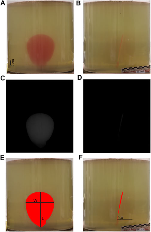
FIGURE 1. Experiment “Dike 1” at time = 190 s. Front and lateral view (Panels A,B). Black and gray images (Panels C,D). Estimated values (Panels E,F). α is the dip of the dike.

Achieving a better understanding of the 3D geometry variations of a flux-driven propagating dike may have important implications in volcanology. For example, prompt detection of the geometric features of a propagating dike through monitoring data may allow estimating the associated energy, providing promising opportunities to expect how far a dike may propagate, ultimately enhancing eruptive hazard assessment (e.g. Bonaccorso et al., 2017).

In this study, we have investigated the variation of the geometric parameters (length, width and thickness) of a continuously fed flux-driven dike as a function of the injection rate. For this goal, we have carried out analogue experiments by injecting water into gelatin.

Methodology

Experimental Set-Up

In our experiments, we injected water (magma analogue) into a pigskin gelatin (type A gelatin, purchased from Italgelatine S.p.A.), selected as the crust analogue material (Kavanagh et al., 2013; Brizzi et al., 2016). The pigskin gelatin solid was prepared at 2.5 wt% by dissolving the appropriate amount of gelatin powder into water at 80°C. We also dissolved 10 wt% of NaCl, so that the gelatin rigidity decreased and the density increased (Brizzi et al., 2016), providing an adequate scaling (see Section Scaling). We poured the solution into a 30 cm diameter cylindrical Plexiglas^® container and filled it up to a height of 30 cm. We cooled the solution in a refrigerator at 8°C for 19 h.

We carried out six experiments injecting water (20°C) at a constant flux from the base of the tank via a tapered-injector using a peristaltic pump. The orientation of the tapered needle allowed us to control the initial orientation of the crack. We used a different injection rate (Q) for each experiment. Q, here used as a proxy of the source pressure (see Section Pressures for details), is the only tested parameter, to understand the variations in the dike geometry during propagation. We focused on the injection rate also as this is an easy and reliable parameter to control and measure with a peristaltic pump.

We monitored the experiments from the side views using two digital cameras, one placed in front of the dike, along its strike, and the other at 90° to the side, acquiring images every 5 s.

Pressures

Following Menand and Tait (2002; and references therein), we consider five pressures to quantitatively characterize our experiments, where a dike is constantly fed. These are:

1) The elastic (or excess) pressure P_e required to contrast the stress perpendicular to a crack and to keep it open. This is expressed by a quasi-static 2D equation (Pollard, 1987; Rubin, 1995)

${\text{P}}_{\text{e}}=\frac{\text{h}}{\text{L}}\frac{\text{G}}{\left(1-\text{ν}\right)}(1)$

where h is the thickness of the dike (i.e. its tensile opening), L is the length of the dike in the direction of propagation (see Figure 1E), G is the shear modulus and ν the Poisson’s coefficient.

2) The source pressure ΔP_r, which is the pressure of the source feeding the dike. Menand and Tait (2002) proposed the following experimental equation, valid for constantly fed dikes (Menand and Tait, 2002):

${\text{ΔP}}_{\text{r}}\sim {\left[\frac{\text{E}{\left(\text{Δ}\rho \text{g}\right)}^2\text{Q}}{2\left(1-{\text{ν}}^2\right)\pi \text{u}}\right]}^{1/3 }(2)$

Where E is the Young modulus of the host rock, Δρ is the density contrast between the host rock and the magma, g is the acceleration due to gravity, Q the volumetric flux of magma injected into the dike, ν the Poisson’s ratio and u is the average velocity of magma inside the dike (i.e. the dike velocity). This formulation has the advantage to relate ΔP_r to the injection rate (Q) and other parameters (u, Δρ), which can be experimentally easily controlled and measured.

3) The buoyancy (or hydrostatic) pressure P_b, due to the density contrast (Δρ) between the host rock and the magma, defined as (Kavanagh et al., 2013):

${\text{P}}_{\text{b}}=\Delta \rho \text{gL}(3)$

4) The viscous pressure drop (P_v), which is the pressure drop due to the viscous flow of the magma within the dike, and is usually negligible in the head of the dike and dominant in the tail (Tait and Taisne, 2013):

${\text{P}}_{\text{v}}\sim \frac{3\eta \text{uL}}{{\left(\text{h}/2\right)}^2}(4)$

where η is the magma viscosity.

5) The fracture pressure (P_f), which is the pressure required to propagate the dike tip and is usually the main resistive pressure acting on the head of the dike (Lister and Kerr, 1991; Menand and Tait, 2002; Rivalta et al., 2015); this is expressed as:

${\text{P}}_{\text{f}}\sim \frac{{\text{K}}_{\text{c}}}{\sqrt{\pi \text{L}}}(5)$

where K_c is the critical fracture toughness.

During dike propagation, ΔP_r and P_b are the main driving pressures acting on the dike, with their sum defined fluid overpressure by Menand and Tait (2002).

The buoyancy pressure (Eq. 3) is the same in all experiments, as we did not change Δρ, whereas the source pressure, directly related to the injection rate Q (Eq. 2), changes with Q in each experiment (Table 1).

TABLE 1

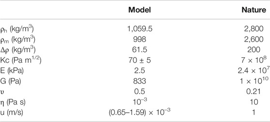
TABLE 1. Mechanical properties of analogue materials and nature. ρ_h = density of the host rock (gelatin in the models); ρ_m density of the magma (water in the models). Δρ is the density contrast. ν is the Poisson’s ratio of the gelatin (model; from Kavanagh et al., 2013) and the host rock (nature; Heap et al., 2009). K_c is the fracture toughness: for the gelatin, K_c has been calculated from the Young modulus (E), using the equation (Kavanagh et al., 2013): ${\text{K}}_{\text{c}}=\left(1.4\pm 0.1\right)\sqrt{\text{E}}$ (E = 2.5 kPa; Sili et al., 2019). Values of K_c in nature are from Gudmundsson, (2009); Rivalta et al., 2015. G is the shear modulus of the host rock (values of E and G in nature are from Heap et al., 2009). η is the viscosity of the water (model) and magma (nature); u is the velocity of the dike (from Traversa et al., 2010 in nature, while for the models it has been directly calculated from the experiments; see Supplementary Figure S1).

Scaling

Model parameters have to be geometrically, kinematically and dynamically scaled, in order to ensure similarities between natural prototypes and experimental results (Merle 2015). Kavanagh et al. 2013 showed that experiments of water injection into gelatin can be appropriately scaled to model dike propagation in nature. The characteristic length scale of the experiments is the buoyancy length L_b, which represents the length over which magma buoyancy driving ascent balances the resistance from rock fracture, defined as (Kavanagh et al., 2013):

${\text{L}}_{\text{b}}={\left(\frac{{\text{K}}_{\text{c}}}{\Delta \rho \text{g}}\right)}^{2/3}(6)$

Where K_c is the fracture toughness of the host material, Δρ is the density difference between the intruded fluid and the host material and g is the acceleration due to gravity (9.8 m/s² in both model and nature). Under the applied experimental conditions (see Section Experimental Set-Up), the mechanical properties of the gelatin and of the injected water, as well as the values that we assume representative of the natural dikes, are reported in Table 2. Therefore, the length scale ${\text{L}}_{\text{b}}^{\text{*}}$ (the asterisk denotes the model to nature ratio) is:

${\text{L}}_{\text{b}}^{\ast }= \frac{{\text{L}}_{\text{b}\_\text{model}}}{{\text{L}}_{\text{b}\_\text{nature}}}=4.73x{10}^{-5}(7)$

imposing that 1 cm in the experiments corresponds to ∼200 m in nature. From the equations proposed by Kavanagh et al. 2013, we calculated also the time scale T* and the velocity scale U*. T* = 7.8*10^–3; U* = 6.2*10^–3. Finally, for the pressure scale we propose both the P_e^* (Table 1) and an adimensional ratio P₁* between the fluid overpressures (ΔP_r + P_b; Menand and Tait, 2002) and the resistive pressure ${\text{P}}_1^{\text{*}}=\left(\Delta {\text{P}}_{\text{r}}^{\text{*}}+{\text{P}}_{\text{b}}^{\text{*}}\right)/\left({\text{P}}_{\text{v}}^{\text{*}}+{\text{P}}_{\text{f}}^{\text{*}}\right)$

TABLE 2

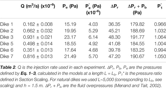
TABLE 2. Injection rate, overpressures and scaling.

As some of these pressures are related to the length L of the dike (see Eqs. 1–5), we calculated them for the experiments at a length equal to L_b (23.8 cm). In Table 1 we report the ${\text{P}}_1^{\text{*}}$ value for each experiment. The values approach 1, implying an appropriate scaling.

Method Limitations

In our experiments we made some assumptions. We neglected solidification effects (Chanceaux and Menand, 2016) and used a single-phase system (water) as analogue of magma, which is usually a three-phase system (liquid + gas + crystals). In addition, the scaling highlights how our experiments simulate the propagation of low viscosity dikes. Therefore, our results are mainly applicable to mafic dikes, widespread in different tectonic settings. Moreover, during each experiment we assumed a constant injection rate, which in nature can change in time (Rivalta, 2010; Rivalta et al., 2015). As we wanted to test the role of the injection rate on the geometry of the propagating dike, we did not change any other possible parameter affecting the dike geometry, such as the viscosity of magma and the mechanical properties of the host rock, which may also vary in nature (Lister and Kerr, 1991; Rivalta et al., 2005; Rivalta and Dahm, 2006; Rivalta et al., 2015).

Image Analysis

We used the Matlab^® image toolbox functions to measure the parameters of the dike such as the length (L), the width (W), the area and the dip (Figure 1). For this, we first subtracted each image with the dike (e. g. Figures 1A,B) to the image without the dike (the master image acquired at time t = 0) in order to obtain an image in which the pixel value is zero (black) in the area without the dike and a positive value (gray) in the area with the dike (Figures 1C,D). Then, this image is converted into a binary image and we measured the parameters of the dike using the Matlab^® function regionprops (Figures 1E,F). The measured length (L, Figure 1E) was then corrected for the dip of the dike (α).

Estimate of the Average Thickness from the Volume/Area Ratio

With the method in section Image Analysis we calculated the area (A) of the dike for each image, which we corrected for the dip of the dike (α). As for each image we also know the associate injected volume (V_i), we measured the average thickness of the dike from the V_i/A ratio.

However, this method has a limitation. As soon as the dike length (L, parallel to the direction of propagation) overcomes a critical value, which depends on the driving and resistive pressures, the dike develops an inflated head followed by a thinner tail (see Rubin, 1995; Rivalta et al., 2015 for details). Once the experimental dike shows a well-developed tail in the second part of each experiment (see Figures 2E,G and Result Section), our method progressively led to an underestimate of the average thickness (Supplementary Figure S2). Indeed, the estimated area of the dike also included the area of the tail, but the injected volume mainly lied within the head (Figures 2E,G). Therefore, to better estimate the average thickness of the dike with a tail, we propose a further method based on the ratio V_head/A_head, where A_head and V_head are respectively the area and the volume and of the dike head. We estimated the area and the volume of the head from the black and gray images (Figure 1C) using the following approach. In the images from the first half of the experiment, with no or a poorly developed tail, the intensity value of each gray pixel (I) associated with the dike showed just a limited variability. As in these images the average thickness (h) estimated with the method V_i/A was almost constant (see result section), we associated that thickness to the average value of the gray intensity (I_a). Knowing the area of the pixel (A_pixel), corrected for the dike dip, we calculated the average volume (V_{pixel_mean}) associated with the average value of the gray intensity using the formula V_{pixel_mean} = A_pixel*h. Then, we associated the gray intensity (I) of each pixel to a volume V_x using equation V_x = (I*V_{pixel_mean})/I_a. To test the validity of this method and its assumptions, we recalculated the total volume of the dike by summing the V_x estimated for each pixel and we compared this value with the real injected volume. As these values were almost equal within a reasonable error (<5%), this method proved reliable. At this point, we applied the calibrated gray scale to calculate the volume within the head of the dike in the images where the dike showed a head and a tail. The area of the head was selected in the summit region in which the gray intensity of the pixels was similar to that shown before the formation of the tail. From the V_head/A_head ratio we calculated the average thickness of the head.

FIGURE 2

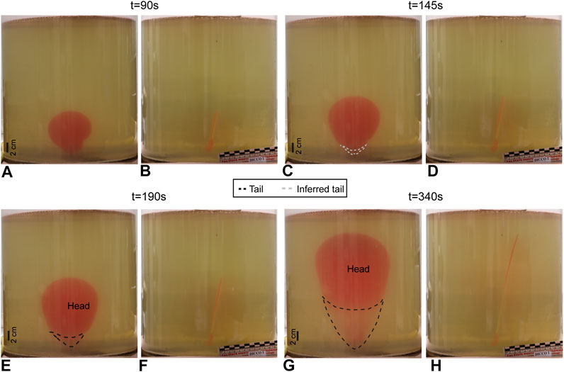
FIGURE 2. Experiment Dike 1. Front (Panels A,C,E,G) and lateral (Panels B,D,F,H) view of the dike during the first (Panels A,B) and second phase (C–H).

Results

Models Description

We briefly describe the first experiment (Dike 1), whose general evolution is representative of all the experiments. When we switch the peristaltic pump on, a sub-vertical water-filled crack forms and propagates. The propagation of our analogue dike can be schematically divided into two main stages, similar to those identified by previous studies with analogous set-up (Menand and Tait, 2002; Kavanagh et al., 2018). At the beginning (first phase), the crack propagates mainly radially in a sub-vertical plane, with sub-circular shape and the length almost equal to the width (Figures 2A,B, 3). In this phase, the crack lacks any preferential direction of propagation (see Figures 2A,B, 3). Then, in the second phase, the crack starts propagating mainly vertically and the length (L) increases faster than the width (W), with the crack assuming an elliptical/inverted teardrop geometry (Figures 2C–H, 3). After few tens of seconds from the onset of the second phase, a thicker head and a thinner tail are clearly identified from the side and front view images (Figures 2E–H).

FIGURE 3

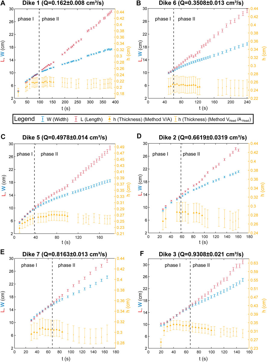
FIGURE 3. Temporal variation of the width (W), length (L) and thickness (h) in each experiment arranged (A–F) with increasing injection rates. The V/A Method is based on the ratio Volume/Area applied in the first phase and at the beginning of the second phase. Then, we apply the method V_head/A_head based on the ratio Volume of the head/Area of the dike head.

The length (L) of the dike at which the transition from the first to the second phase occurs is proportional to the injection rate of the experiment (Figure 3) and ranges from ∼10 cm in the experiment at the lowest injection rate to ∼16 cm in the experiment at the highest rate (Figure 3). In addition, the front and side view images suggest that in the higher Q experiments the amount of magma left over in the tail increases (see images in the data repository Galetto, 2021).

Dike Thickness (h)

Figure 3 reports the temporal variation of the average thickness of the crack in each experiment. For the first and second phase, we used the method based on the Volume/Area ratio. At the onset of injection (beginning of phase one), when the dike nucleates, the thickness quickly increases with time. Then, the thickness remains approximately constant until the end of the experiment. After few tens of seconds from the onset of the second phase, when the images of the experiments show a thicker head and a thinner tail, we start measuring the thickness with the method V_head/A_head based on the color intensity to avoid the possibility that the tail overestimates the area, leading to an underestimate in the thickness (which would linearly decrease with time). With the V_head/A_head method, we find that the thickness of the head remains almost constant until the end of the experiment. However, there is a small drop in the average thickness at the transition between the two methods, when the tail becomes identifiable; this drop is negligible in the three experiments at lower Q, whereas it is slightly more evident in the three experiments at higher Q.

The results highlight two main aspects related to the thickness of the dike: i) this is proportional to the injection rate, here used as a proxy of the source pressure (ΔP_r) (Figure 4A and Table 1); ii) after a short initial stage of growth, the thickness remains approximately constant. In addition, Figure 4B shows that in each experiment the thickness/length ratio (h/L) and the related P_e (see Eq. 1), calculated for the same L of the dike, are also directly proportional to the injection rate. According to Pollard (1987) and Rubin and Pollard (1987), we calculated P_e using the length L parallel to the direction of propagation of the dike. Some Authors (e.g. Lister and Kerr, 1991) proposed to consider the shortest dimension between L and W (which would be W in our models), and using the h/W ratio we obtain the same linear correlation with P_e (see Supplementary Figure S3). Finally, the P_e calculated in each experiment for equal intruded volumes (but different length) is again proportional to Q (Figure 4C).

FIGURE 4

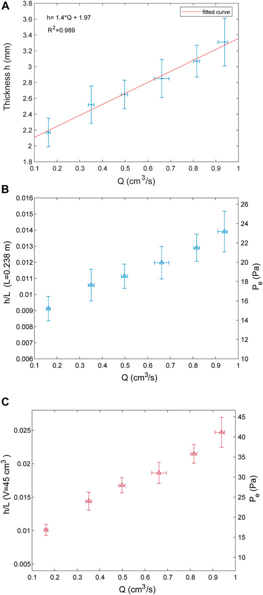
FIGURE 4. (A) Thickness of the dike as a function of the injection rate (Q). (B) Variation of the thickness/length ratio (h/L) and the associated P_e as a function of the injection rate (Q). In each experiment h/L and P_e have been calculated when the dikes reach the same length (L = L_b = 0.238 m; see equation 6) (C) Variation of h/L and P_e as a function of Q, calculated by intruding the same amount of Volume (V = 45 cm³).

Dike Width (W)

Figure 3 shows the temporal variation of the dike width W in each experiment. During the first phase, the width increases almost linearly. Then, during the second phase, it still increases linearly, but at a slower rate. The fact that in the final part of the experiments, where the dikes are wider, we do not observe any decrease in the velocity of growth of the width of the dike, suggests that any possible border effect of the Plexiglas^® container is negligible.

Results highlight that the dike width is proportional to the injected volume, whereas there is no clear relationship with the variation in the injection rate (Figure 5). Therefore, similar dike widths are reached with the same injected volumes, even at different injection rates.

FIGURE 5

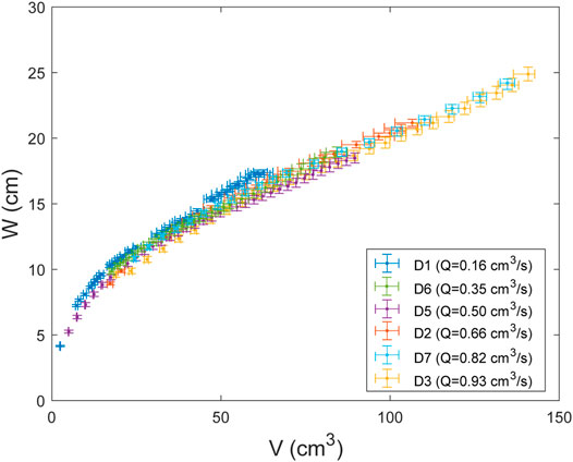
FIGURE 5. Variation of the dike width with the intruded volume (V). D1, D2, D3, D5, D6, D7 point respectively Experiments 1, 2, 3, 5, 6, 7.

Finally, the total volume injected when the dike erupts is proportional to the injection rate (Figure 6A). Therefore, the final maximum width of the dike, when this erupts (W_er), is also somehow proportional to the injection rate (Figure 6B), as a higher rate will generate a dike with larger volume that in turn is related to a larger width.

FIGURE 6

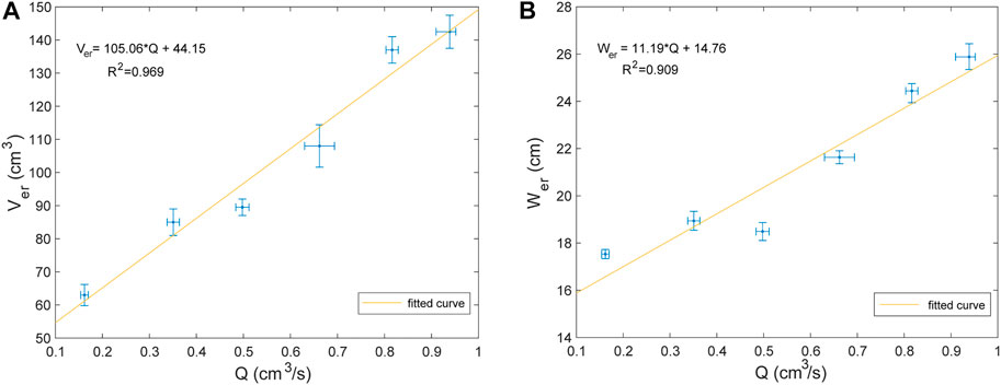
FIGURE 6. A) Total intruded volume at the moment of eruption (V_er) as a function of the injection rate. (B) Width of the dike at the moment of eruption (W_er) as a function of the injection rates.

Discussion

General Features

Our models reproduce near vertical dikes fed by a constant injection rate (Q). During the propagation, we observe different relationships between the geometry of the dike (L, W, and h) and the injection rate. During the first phase, the length and width of the dike grow about at the same rate and the thickness soon approaches a constant value. Then, during the second phase, the dike starts propagating vertically faster than laterally, while the thickness remains almost constant, although there may be a minor drop when the tail appears (Figure 3). These behaviors are explained considering the pressures acting on the dike (Figure 7A) (Menand and Tait, 2002). During the first phase, the resistive pressures, mostly related to the fracture pressure P_f, are higher than the fluid overpressure (P_b + ΔP_r) driving dike propagation (Figure 7B) and indeed the dike grows radially, without any preferred direction. At the beginning of the second phase, the fluid overpressure approaches and then overcomes P_f, mainly because of the increase of P_b, that becomes the main driving component, and the dike starts propagating mostly upward (Figure 7B; Menand and Tait, 2002). This explains why L increases faster than W (Menand and Tait, 2002). The progressive decrease of P_f and P_e (Figure 7A) is expected by the linear elastic theory, as, the longer the dike, the lower the energy P_f required to propagate its tip, and the lower the elastic energy P_e required to keep the fracture open (e.g. Rubin and Pollard, 1987; Rubin, 1995). Figure 7A also shows that during the propagation of a constantly fed dike the viscous pressure drop is a negligible resistive pressure at the dike head, in agreement with theoretical models (Lister and Kerr, 1991; Tait and Taisne, 2013). Finally, the small drop in the thickness of the dike head at the appearance of the tail (Figure 3) may be related to the amount of fluid left over in the tail (Rivalta et al., 2015). This is supported by the fact that this drop is negligible in the experiments at lower injection rate, where the dike tail is almost closed, while it becomes more evident in the experiments at higher rate, with thicker tail (see data in Galetto, 2021). The fact that the amount of magma left over in the tail increases with the injection rate Q, as suggested by the front and side images, is expected by fluid-mechanical models of crack propagation (see Lister and Kerr, 1991 for a detailed analysis).

FIGURE 7

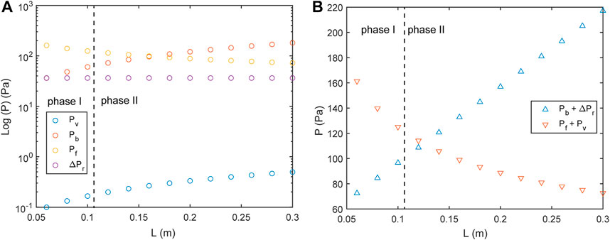
FIGURE 7. A) Variation of the pressures as a function of the length of the dike in experiment “Dike 1” (Q = 0.162 ± 0.008 cm³/s). P_e, P_v, P_b, P_f, and ΔP_r are the elastic pressure, the viscous pressure drop, the buoyancy pressure, the fracture pressure and the source pressure, respectively (see equation 2–5). (B) Variation of the fluid overpressure (P_b + ΔP_r) and of the resistive pressure (P_f + P_v) as a function of the dike length in “Dike 1”.

New Insights on Dike Thickness and Width

Our experiments show a different behavior of the thickness and the width of the dikes with respect to the injection rate and volume change. A first important aspect is that the thickness h tends to remain approximately constant during dike propagation. The fact that after the minor drop at the appearance of the tail the thickness of the head remains almost constant also confirms that under the applied experimental conditions the thickness does not change in time. Therefore, the total injected volume, which increases with time, does not seem to influence the thickness. On the contrary, the thickness is directly proportional to the injection rate Q, here used as a proxy of the source pressure ΔP_r (Figure 4A and Table 1; Menand and Tait, 2002).

Another important point is that the buoyancy pressure (P_b) does not affect the dike thickness. Indeed P_b (see Eq. 3) increases with the length of the dike in each experiment (Figure 7A), whereas the thickness remains constant. The experiments also highlight that a higher Q (i.e. higher ΔP_r) generates a higher h/L ratio and therefore higher P_e (Figures 4A,B), in agreement with the linear elastic theory (Pollard, 1987; Rubin, 1995).

A novelty revealed by the experiments is that, contrary to the thickness, the dike width is proportional to the injected volume, and therefore increases over time, whereas there is no clear relationship with the injection rate (Figure 5). This new aspect shows that similar crack widths are obtained when same crack volumes are injected, even with different injection rate. Under the applied experimental conditions, the volume of the dike and the P_b progressively grow. Taisne et al. 2011 found a relationship between the buoyancy force, the volume, and width of the dike (see equation 12 in Taisne et al., 2011) for buoyancy-driven dikes. Their equation derives from the balance between the fracture and buoyancy pressures, as their buoyancy-driven dikes resulted from a limited volume of magma rising only for buoyancy. By using their equation, we may estimate the contribution of the buoyancy to the dike width in our models. The difference between our measured dike width and the buoyancy width estimated following Taisne et al. 2011 should be the contribution to the width due to the constant injection (Figure 8), which is the only driving force in our models that is absent in Taisne et al. 2011. This suggests that even if the width of the dike mainly depends on the injected volume, for equal injected volumes the two widths may differ depending on whether the dike is continuously fed (flux-driven dike) or not (buoyancy-driven dike) from its source.

FIGURE 8

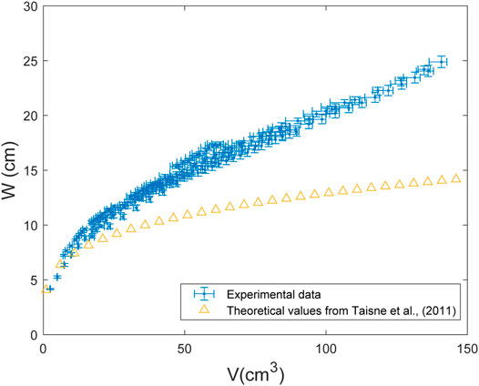
FIGURE 8. Variation of the dike width (W) with the intruded volume (V) in our models (flux-driven dike; blue crosses) and as predicted by Taisne et al., (2011) for buoyancy driven dikes (orange triangles).

Comparison to Natural Dikes and Implications

According to our results, a constantly fed dike increases its width over time, but not its thickness, if the injection rate remains constant. On the contrary, if the injection rate increases, the thickness also increases. Thus, during dike propagation any volume change does not necessarily imply a variation in all the geometric parameters of the dike.

A first main novelty of our experiment regards the dike thickness. Our results confirm that thicker dikes are related to higher source pressures, and therefore they will release more energy. This agrees with Bonaccorso et al. (2017), who found a simple but effective equation that relates the squared value of the dike thickness with the expected released mechanical energy and, in turn, to the recorded seismic moment produced by the earthquakes associated with dike propagation. These Authors showed that the available mechanical elastic strain energy has to be entirely released seismically, and this can be preliminarily estimated by the dike thickness. This means that the dike thickness is the most important and unequivocal parameter related to the energy to be released and, therefore, from the comparison between the expected energy and the recorded released seismicity, it may possible to evaluate in real-time the state of the propagating dike (Bonaccorso et al., 2017). This general approach was retrospectively applied to two recent dike intrusions feeding flank eruptions at Etna volcano on October 2002 (Bonaccorso et al., 2017) and December 2018 (Bonaccorso and Giampiccolo, 2020). In this rationale, a crucial aspect concerns the hypothesis that the thickness of the dike remains approximately constant during its propagation, which is a feature that has never been proven so far and that is now confirmed by our models (if injection rates do not change significantly). Furthermore, it is also interesting to note that the modeling of the continuous ground deformation data (borehole tilt and GPS) modeled over time of the 2002 (Aloisi et al., 2006) and 2018 eruptions (Aloisi et al., 2020) suggested a near constant thickness during the dike propagation, as expected by our experiments.

Our results show that a constantly fed dike should propagate varying its width and volume, but not the thickness. Conversely, any increase in the thickness would imply an increase in the injection rate. Nevertheless, if the width of a propagating dike does not change significantly, the dike would not be continuously fed from its source and would be propagating only through buoyancy (Taisne et al., 2011). Some examples of well-studied propagating dikes in nature support these findings. For example, at Cerro Azul (Galápagos) in 2008 a propagating radial dike underwent a sudden increase in the injection rate and volume, also increasing its thickness and width (Galetto et al., 2020). Similarly, the increase in width and thickness of the 2014 Bárðarbunga dike (Iceland) mainly occurred at the onset of its propagation, when the increase in volume change and injection rate were higher (Sigmundsson et al., 2015; Heimisson and Segall, 2020).

Finally, our results may allow reinterpretation of previous eruptive events. In fact, the relationship between the thickness and injection rate in flux-driven dikes implies that the greater the thickness the higher the injection rate of the dike and, as the injection rate is a proxy of the source pressure (Menand and Tait, 2002), the higher the source pressure. This relationship is particularly useful, as direct estimation of the source pressure feeding a dike is difficult (if not impossible) and even the estimation of injection rate may be difficult if geodetic data are not detected in a continuous mode. For example, the 2005–2009 sequence of rifting at the Manda-Hararo Rift (Afar, Ethiopia) was triggered by the intrusion of at least thirteen dikes. Although the 3D geometry has been estimated for all these dikes (Hamling et al., 2009; Grandin et al., 2010), their injection rates remain unknown. Using our approach, it may be possible to establish a hierarchy of the dikes fed by the highest and lowest injection rates (and source pressures), simply based on their thickness. These possible in-depth studies are beyond the scope of our work, although we believe they may be useful to further explore the potential for applying the results of our experiments.

Our results highlight the importance of studying the 3D geometry variation during dike propagation. Future studies should investigate whether any other parameter (e.g. viscosity, Young’s modulus and cooling) may also affect the geometry of a propagating dike.

Conclusion

Our models show that in experimental flux-driven dikes:

1) Dike thickness is related to the injection rate and therefore to the source pressure ΔP_r, whereas it does not seem to be related to buoyancy pressure.

2) Dike thickness tends to remain constant if injection rate does not change.

3) Higher injection rates (i.e. higher ΔPr) generate higher h/L ratios and therefore higher elastic pressures (Figures 4B,C), as expected from the linear elastic theory.

4) Similar crack widths are obtained when same volumes are injected, even with different injection rates.

These results increase our understanding of the 3D geometric variation during the propagation of a dike continuously fed from its source and are consistent with the behavior inferred from observations of several historically emplaced dikes. In addition, our results offer new opportunities to better understand how dikes propagated during previous events and also how propagation will proceed for dikes with geometry delineated by real-time monitoring during an emplacement event.

Data Availability Statement

The original contributions presented in the study are included in the article/Supplementary Material. Images of the analogue experiments are available in the data repository https://doi.org/10.17605/OSF.IO/Z42PH (Galetto, 2021). Further inquiries can be directed to the corresponding authors.

Author Contributions

AB conceived this work and traced its scheme. FG carried out the experiments and processed the data. VA supervised the experiments. All the authors contributed with original ideas to the drafting of the article and shared the discussion of the results.

Conflict of Interest

The authors declare that the research was conducted in the absence of any commercial or financial relationships that could be construed as a potential conflict of interest.

Acknowledgments

We thank Fabio Corbi, Stefano Urbani and Eleonora Rivalta for their help with the experimental set-up and the scaling. FG is grateful to Matteo Galetto for assistance in developing the method based on the color intensity and for developing the associated Matlab^® code. FG was supported by the INGV project Premiale-MIUR acronym “Transienti”. We thank S. Conway for improving the quality of the English. We thank the Editor J. White and two anonymous Reviewers whose comments significantly improved the quality of this manuscript.

Supplementary Material

The Supplementary Material for this article can be found online at: https://www.frontiersin.org/articles/10.3389/feart.2021.665865/full#supplementary-material

References

Aloisi, M., Bonaccorso, A., Cannavò, F., Currenti, G., and Gambino, S. (2020). The 24 December 2018 Eruptive Intrusion at Etna Volcano as Revealed by Multidisciplinary Continuous Deformation Networks (CGPS, Borehole Strainmeters and Tiltmeters). J. Geophys. Res. Solid Earth 125, e2019JB019117. doi:10.1029/2019jb019117

CrossRef Full Text | Google Scholar

Aloisi, M., Bonaccorso, A., and Gambino, S. (2006). Imaging Composite Dike Propagation (Etna 2002, Case). J. Geophys. Res. 111, B06404. doi:10.1029/2006jb004616

CrossRef Full Text | Google Scholar

Bonaccorso, A., Aoki, Y., and Rivalta, E. (2017). Dike Propagation Energy Balance from Deformation Modeling and Seismic Release. Geophys. Res. Lett. 44, 5486–5494. doi:10.1002/2017gl074008

CrossRef Full Text | Google Scholar

Bonaccorso, A., and Giampiccolo, E. (2020). Balance between Deformation and Seismic Energy Release: The Dec 2018 ‘Double-Dike’ Intrusion at Mt. Etna. Front. Earth Sci. 8, 583815. doi:10.3389/feart.2020.583815

CrossRef Full Text | Google Scholar

Brizzi, S., Funiciello, F., Corbi, F., Di Giuseppe, E., and Mojoli, G. (2016). Salt Matters: How Salt Affects the Rheological and Physical Properties of Gelatine for Analogue Modelling. Tectonophysics. 679, 88–101. doi:10.1016/j.tecto.2016.04.021

CrossRef Full Text | Google Scholar

Cañón-Tapia, E., and Merle, O. (2006). Dyke Nucleation and Early Growth from Pressurized Magma Chambers: Insights from Analogue Models. J. Volcanology Geothermal Res. 158, 207–220. doi:10.1016/j.jvolgeores.2006.05.003

CrossRef Full Text | Google Scholar

Chanceaux, L., and Menand, T. (2016). The Effects of Solidification on Sill Propagation Dynamics and Morphology. Earth Planet. Sci. Lett. 442, 39–50. doi:10.1016/j.epsl.2016.02.044

CrossRef Full Text | Google Scholar

Daniels, K. A., Kavanagh, J. L., Menand, T., and R. Stephen, J. S. (2012). The Shapes of Dikes: Evidence for the Influence of Cooling and Inelastic Deformation. Geol. Soc. America Bull. 124, 1102–1112. doi:10.1130/b30537.1

CrossRef Full Text | Google Scholar

Galetto, F., Hooper, A., Bagnardi, M., and Acocella, V. (2020). The 2008 Eruptive Unrest at Cerro Azul Volcano (Galápagos) Revealed by InSAR Data and a Novel Method for Geodetic Modelling. J. Geophys. Res. Solid Earth. 125 (2), e2019JB018521. doi:10.1029/2019jb018521

CrossRef Full Text | Google Scholar

Galetto, F. (2021). New Insights on Dikes’ Shape Properties during Their Propagation in Analogue Flux-Driven Experiments. doi:10.17605/OSF.IO/Z42PH

CrossRef Full Text | Google Scholar

Geshi, N., Browning, J., and Kusumoto, S. (2020). Magmatic Overpressures, Volatile Exsolution and Potential Explosivity of Fissure Eruptions Inferred via Dike Aspect Ratios. Scientific Rep. 10, 1–9. doi:10.1038/s41598-020-66226-z

PubMed Abstract | CrossRef Full Text | Google Scholar

Grandin, R., Socquet, A., Jacques, E., Mazzoni, N., de Chabalier, J.-B., and King, G. C. P. (2010). Sequence of Rifting in Afar, Manda-Hararo Rift, Ethiopia, 2005-2009: Time-Space Evolution and Interactions between Dikes from Interferometric Synthetic Aperture Radar and Static Stress Change Modeling. J. Geophys. Res. 115, B10413. doi:10.1029/2009jb000815

CrossRef Full Text | Google Scholar

Gudmundsson, A. (2002). Emplacement and Arrest of Sheets and Dykes in Central Volcanoes. J. Volcanology Geothermal Res. 116, 279–298. doi:10.1016/s0377-0273(02)00226-3

CrossRef Full Text | Google Scholar

Gudmundsson, A. (2009). Toughness and Failure of Volcanic Edifices. Tectonophysics 471, 27–35. doi:10.1016/j.tecto.2009.03.001

CrossRef Full Text | Google Scholar

Hamling, I. J., Ayele, A., Bennati, L., Calais, E., Ebinger, C. J., Keir, D., et al. (2009). Geodetic Observations of the Ongoing Dabbahu Rifting Episode: New Dyke Intrusions in 2006 and 2007. Geophys. J. Int. 178, 989–1003. doi:10.1111/j.1365-246x.2009.04163.x

CrossRef Full Text | Google Scholar

Heap, M. J., Vinciguerra, S., and Meredith, P. G. (2009). The Evolution of Elastic Moduli with Increasing Crack Damage during Cyclic Stressing of a Basalt from Mt. Etna Volcano. Tectonophysics. 471, 153–160. doi:10.1016/j.tecto.2008.10.004

CrossRef Full Text | Google Scholar

Heimisson, E. R., and Segall, P. (2020). Physically Consistent Modeling of Dike-Induced Deformation and Seismicity: Application to the 2014 Bárarbunga Dike, Iceland. J. Geophys. Res. Solid Earth 125, e2019JB018141. doi:10.1029/2019JB018141

CrossRef Full Text | Google Scholar

Heimpel, M., and Olson, P. (1994). “Chapter 10 Buoyancy-Driven Fracture and Magma Transport through the Lithosphere: Models and Experiments,” in Buoyancy-Driven Fracture and Magma Transport through the Lithosphere: Models and Experiments. Editor M. Ryan (New York: Magmatic Systems, Academic Press), 223–240. doi:10.1016/s0074-6142(09)60098-x

CrossRef Full Text | Google Scholar

Kavanagh, J. L., Burns, A. J., Hilmi Hazim, S., Wood, E. P., Martin, S. A., Hignett, S., et al. (2018). Challenging Dyke Ascent Models Using Novel Laboratory Experiments: Implications for Reinterpreting Evidence of Magma Ascent and Volcanism. J. Volcanology Geothermal Res. 354, 87–101. doi:10.1016/j.jvolgeores.2018.01.002

CrossRef Full Text | Google Scholar

Kavanagh, J. L., Menand, T., and Daniels, K. A. (2013). Gelatine as a Crustal Analogue: Determining Elastic Properties for Modelling Magmatic Intrusions. Tectonophysics. 582, 101–111. doi:10.1016/j.tecto.2012.09.032

CrossRef Full Text | Google Scholar

Kavanagh, J. L., and Sparks, R. S. J. (2011). Insights of Dyke Emplacement Mechanics from Detailed 3D Dyke Thickness Datasets. J. Geol. Soc. 168, 965–978. doi:10.1144/0016-76492010-137

CrossRef Full Text | Google Scholar

Lister, J. R., and Kerr, R. C. (1991). Fluid-mechanical Models of Crack Propagation and Their Application to Magma Transport in Dykes. J. Geophys. Res. 96 (10), 10049–10077. doi:10.1029/91jb00600

CrossRef Full Text | Google Scholar

Menand, T., and Tait, S. (2002). The Propagation of a Buoyant Liquid-Filled Fissure from a Source under Constant Pressure: An Experimental Approach. J. Geophys. Res. 107 (B11), 2306. doi:10.1029/2001jb000589

CrossRef Full Text | Google Scholar

Merle, O. (2015). The Scaling of Experiments on Volcanic Systems. Front. Earth Sci. 3, 26. doi:10.3389/feart.2015.00026

CrossRef Full Text | Google Scholar

Morita, Y., Nakao, S., and Hayashi, Y. (2006). A Quantitative Approach to the Dike Intrusion Process Inferred from a Joint Analysis of Geodetic and Seismological Data for the 1998 Earthquake Swarm off the East Coast of Izu Peninsula, Central Japan. J. Geophys. Res. 111, a–n. doi:10.1029/2005jb003860

CrossRef Full Text | Google Scholar

Pollard, D. D. (1987). “Elementary Fracture Mechanics Applied to the Structural Interpretation of Dykes,”in Mafic Dyke Swarms, Geol. Assoc. Canada. Editor H. C. Halls (W. H. Fahrig), Vol. 34, 112–128.

Google Scholar

Pollard, D. D., and Muller, O. H. (1976). The Effect of Gradients in Regional Stress and Magma Pressure on the Form of Sheet Intrusions in Cross Section. J. Geophys. Res. 81, 5. doi:10.1029/jb081i005p00975

CrossRef Full Text | Google Scholar

Rivalta, E., Böttinger, M., and Dahm, T. (2005). Buoyancy-driven Fracture Ascent: Experiments in Layered Gelatine. J. Volcanology Geothermal Res. 144, 273–285. doi:10.1016/j.jvolgeores.2004.11.030

CrossRef Full Text | Google Scholar

Rivalta, E., and Dahm, T. (2006). Acceleration of Buoyancy-Driven Fractures and Magmatic Dikes beneath the Free Surface. Geophys. J. Int. 166, 1424–1439. doi:10.1111/j.1365-246x.2006.02962.x

CrossRef Full Text | Google Scholar

Rivalta, E. (2010). Evidence that Coupling to Magma Chambers Controls the Volume History and Velocity of Laterally Propagating Intrusions. J. Geophys. Res. Solid Earth 115. doi:10.1029/2009jb006922

CrossRef Full Text | Google Scholar

Rivalta, E., Taisne, B., Bunger, A. P., and Katz, R. F. (2015). A Review of Mechanical Models of Dike Propagation: Schools of Thought, Results and Future Directions. Tectonophysics. 638, 1–42. doi:10.1016/j.tecto.2014.10.003

CrossRef Full Text | Google Scholar

Rubin, A. M., and Pollard, D. D. (1987). “Origins of Blade-like Dikes in Volcanic Rift Zones,” in Volcanism in Hawaii, U.S. Geol. Surv. Prof. Pap., 1350. Editors R. D. Decker, T. L. Wright, and P. H. Stauffer (Washington, DC: US geological survey professional paper), 1449–1470.

Google Scholar

Rubin, A. M. (1995). Propagation of Magma-Filled Cracks. Annu. Rev. Earth Planet. Sci. 23, 287–336. doi:10.1146/annurev.ea.23.050195.001443

CrossRef Full Text | Google Scholar

Segall, P., Cervelli, P., Owen, S., Lisowski, M., and Miklius, A. (2001). Constraints on Dike Propagation from Continuous GPS Measurements. J. Geophys. Res. 106 (19), 19301–19317. doi:10.1029/2001jb000229

CrossRef Full Text | Google Scholar

Sigmundsson, F., Hooper, A., Hreinsdóttir, S., Vogfjörd, K. S., Ófeigsson, B. G., Heimisson, E. R., et al. (2015). Segmented Lateral Dyke Growth in a Rifting Event at Bárarbunga Volcanic System, Iceland. Nature 517, 191–195. doi:10.1038/nature14111

CrossRef Full Text | Google Scholar

Sili, G., Urbani, S., and Acocella, V. (2019). What Controls Sill Formation: An Overview from Analogue Models. J. Geophys. Res. Solid Earth 124, 8205–8222. doi:10.1029/2018jb017005

CrossRef Full Text | Google Scholar

Taisne, B., Tait, S., and Jaupart, C. (2011). Conditions for the Arrest of a Vertical Propagating Dyke. Bull. Volcanol. 73, 191–204. doi:10.1007/s00445-010-0440-1

CrossRef Full Text | Google Scholar

Tait, S., and Taisne, B. (2013). The Dynamics of Dike Propagation. in Modeling Volcanic Processes: The Physics and Mathematics of Volcanism. Editor S A Fagents (Cambridge, United Kingdom: Cambridge University Press), 33–54.

Google Scholar

Takada, A. (1990). Experimental Study on Propagation of Liquid-Filled Crack in Gelatin: Shape and Velocity in Hydrostatic Stress Condition. J. Geophys. Res. 95, 8471–8481. doi:10.1029/jb095ib06p08471

CrossRef Full Text | Google Scholar

Traversa, P., Pinel, V., and Grasso, J. R. (2010). A Constant Influx Model for Dike Propagation: Implications for Magma Reservoir Dynamics. J. Geophys. Res. 115, B01201. doi:10.1029/2009jb006559

CrossRef Full Text | Google Scholar

Urbani, S., Acocella, V., Rivalta, E., and Corbi, F. (2017). Propagation and Arrest of Dikes under Topography: Models Applied to the 2014 Bardarbunga (Iceland) Rifting Event. Geophys. Res. Lett. 44, 6692–6701. doi:10.1002/2017gl073130

CrossRef Full Text | Google Scholar

Urbani, S., Acocella, V., and Rivalta, E. (2018). What Drives the Lateral versus Vertical Propagation of Dikes? Insights from Analogue Models. J. Geophys. Res. Solid Earth. 123, 3680–3697. doi:10.1029/2017jb015376

CrossRef Full Text | Google Scholar