Evolution of Surface Characteristics of Three Debris-Covered Glaciers in the Patagonian Andes From 1958 to 2020

Introduction

Driven by climate change, glaciers in most high mountain ranges around the globe are receding and losing mass rapidly (Jomelli et al., 2011; Davies and Glasser, 2012; Zekollari et al., 2019; Davaze et al., 2020; Hugonnet et al., 2021). Whilst glaciers steadily thin and contribute to sea level rise through increased melting (Zemp et al., 2019), another aspect of glacier change and adjustment to drier conditions is the progressive accumulation of surface debris stemming from the surrounding valley walls and lateral moraines (Scherler et al., 2011; Kirkbride and Deline, 2013; Sasaki et al., 2016; Tielidze et al., 2020). Debris cover on glacier surfaces accounts for ∼7% of the mountain glacier area worldwide (Herreid and Pellicciotti, 2020), and is relevant from a surface energy balance point of view, as the distribution and thickness variability of debris layers can alter glacier melt rates (Nicholson et al., 2018; Fyffe et al., 2020). Length adjustments and overall response times of debris-covered glaciers to climate variability are often delayed compared to debris-free glaciers. This delayed signal can occur as ablation rates decrease when debris layers are thicker than the effective thickness (i.e. the thickness above which glacier ice is sheltered and insulated from solar radiation, commonly <0.1 m; Mattson, 2000; Mihalcea et al., 2008; Reznichenko et al., 2010). Normally, the thickness of debris layers increases toward the glacier terminus, resulting in lower or even reversed mass balance gradients (e.g. Benn et al., 2012; Rounce et al., 2018; Bisset et al., 2020).

The spatio-temporal relationship between debris cover, surface mass balance glacier dynamics is nevertheless not simple. The mass balance gradient of debris-covered glaciers may not vary in straightforward form with elevation, and debris-covered glaciers are said to react by thinning or thickening in response to climate forcing rather than terminus recession or advance due to their typically gentle slopes (Bolch et al., 2008; Pellicciotti et al., 2015). Reduced ablation on the debris-covered portions of glaciers can result in a decrease in overall slope, which subsequently favors a reduction in ice flow velocities (Rowan et al., 2015; Dehecq et al., 2019). A feedback mechanism is established whereby rising Equilibrium Line Altitudes (ELA) lead to an earlier melt out and emergence of englacial debris, extending the debris layer further up-glacier. In this way, the overall glacier slope is additionally reduced, leading to stagnation of the glacier tongues (Quincey et al., 2009; Benn et al., 2012; Haritashya et al., 2015). Surface and basal ice melt, coupled with surface lowering, culminate in the formation and expansion of supraglacial lakes, causing further enhancement of glacier ablation (Mertes et al., 2017).

In spite of the above, more than a few studies, particularly in the Himalayas, have shown that debris-covered glaciers can have surface lowering rates comparable to those of debris-free glaciers (Kääb et al., 2012; Ragettli et al., 2016; King et al., 2019). A number of causes for this uncertainty have been identified so far (see e.g. Mölg et al., 2019 and references therein), including the influence of ice cliffs. Ice cliffs are steeply inclined areas of glacier ice, usually covered only by a very thin layer of debris, that vary from sub-circular to largely elongated in shape, and are of varying size (Sakai et al., 2002; Steiner et al., 2019). The occurrence of exposed ice in otherwise predominantly debris-covered glacier surfaces in the form of cliffs and supraglacial ponds (often associated) can boost ablation in comparison to “regular” debris-covered surfaces or even debris-free areas (Sakai et al., 1998; Sakai et al., 2002; Juen et al., 2014). The influence of ice cliffs and supraglacial ponds on the evolution of debris-covered glaciers is presently well acknowledged and the mapping and monitoring of these cryokarst forms has increased in recent years (Buri et al., 2016; Watson et al., 2017; Herreid and Pellicciotti, 2018; Mölg et al., 2019; Steiner et al., 2019; Ferguson and Vieli, 2020).

Bolch et al. (2012) pointed out that understanding the interactions between debris cover, mass balance and glacier dynamics would be a major achievement for envisaging the future evolution of debris-covered glaciers in high mountain areas. Consequently, recent studies have attempted to integrate this subject by assimilating diverse glacier variables (mass balance, debris distribution, thickness and transport, flow rates) and their feedback mechanisms into numerical models (Banerjee and Shankar, 2013; Collier et al., 2015; Rowan et al., 2015; Anderson and Anderson, 2018). Although large-scale assessments on debris-covered ice worldwide distribution exist (Scherler et al., 2018), modeling efforts are currently limited by the relative scarcity of more specific debris-covered glacier data, such as debris thickness and the evolution of ice cliffs and supraglacial ponds. These parameters are available mostly for the Himalaya, Karakorum, (e.g. Han et al., 2010; Thompson et al., 2012; Brun et al., 2018; Nicholson et al., 2018; Rounce et al., 2018; Buri et al., 2021) and to a lesser degree the European Alps (Reid and Brock, 2014; Mölg et al., 2019), but are lacking for other mountain regions where debris-covered glaciers are common (Röhl, 2006). In the Andes of Argentina and Chile, specifics about the evolution of debris layers, and their influence in glacier surface morphology, overall dynamics and mass changes, is particularly limited despite the abundance of debris-covered ice in some sectors such as the Central Andes (see e.g. Bodin et al., 2010; Wilson et al., 2016a; Falaschi et al., 2018; Ferri et al., 2020). In comparison to the Central Andes, however, the Patagonian Andes show a much lower relative concentration of debris-covered glaciers (Falaschi et al., 2013; Masiokas et al., 2015), although debris-covered ice can be relevant in some specific sites. Specifically for the Río Mayer catchment, debris-covered ice accounts for ∼15% of the total glacier area (IANIGLA, 2018). In addition, recent studies have detected signs of increasing proportions of debris-covered ice in the large outlet glaciers from the Patagonian Icefields in recent decades (Glasser et al., 2016).

In this study, we aim to determine the main characteristics of the morphological features of the Río Oro, Río Lácteo and San Lorenzo Sur debris-covered glaciers in the eastern (Argentinian) side of the Monte San Lorenzo massif (Southern Patagonian Andes), namely the distribution and area changes of the debris layer, ice cliffs and supraglacial ponds from 1958 to 2020. In addition, we produce the most complete glacier velocity record from freely available (mostly Landsat) satellite imagery. Whilst the mass balance evolution of these glaciers has been strongly linked to climate variability, proglacial lakes influence glacier evolution to a significant extent as well (Falaschi et al., 2019). Additionally, these three glaciers have one of the longest (geodetic) mass balance records in the Southern Andes and have been studied previously in regards to their geometric evolution. Combining the newly produced datasets and mass balance and climate records previously available, we discuss the spatio-temporal interactions between surface features and glacier velocities, and the likely impact on mass balance evolution. Finally, we evaluate the possible linkage between the observed areal evolution of the debris-covered area in view of the late-summer snowline elevation and climate variability in the area.

Study Area and Previous Studies

Río Oro, Río Lácteo, and San Lorenzo Sur valley glaciers (Figure 1; Supplementary Table S1) lie on the Argentinian side of Monte San Lorenzo (47°35′S, 72°18′W; 3,706 m asl), the second highest peak in Southern Patagonia, ∼70 km East of the southernmost tip of the Northern Patagonian Icefield. At these latitudes, the Andes act as an effective orographic barrier to the humid westerly flow (Rivera et al., 2007), producing steep meteorological gradients and a strong rain shadow effect to the east of the main water divide (Bravo et al., 2019; Sauter, 2020). In fact, whilst the Northern Patagonian Icefield has a clear maritime climatic regime and receives extreme precipitation (Lenaerts et al., 2014), the San Lorenzo area lies in a more transitional environment and receives much less precipitation (Damseaux et al., 2020).

FIGURE 1

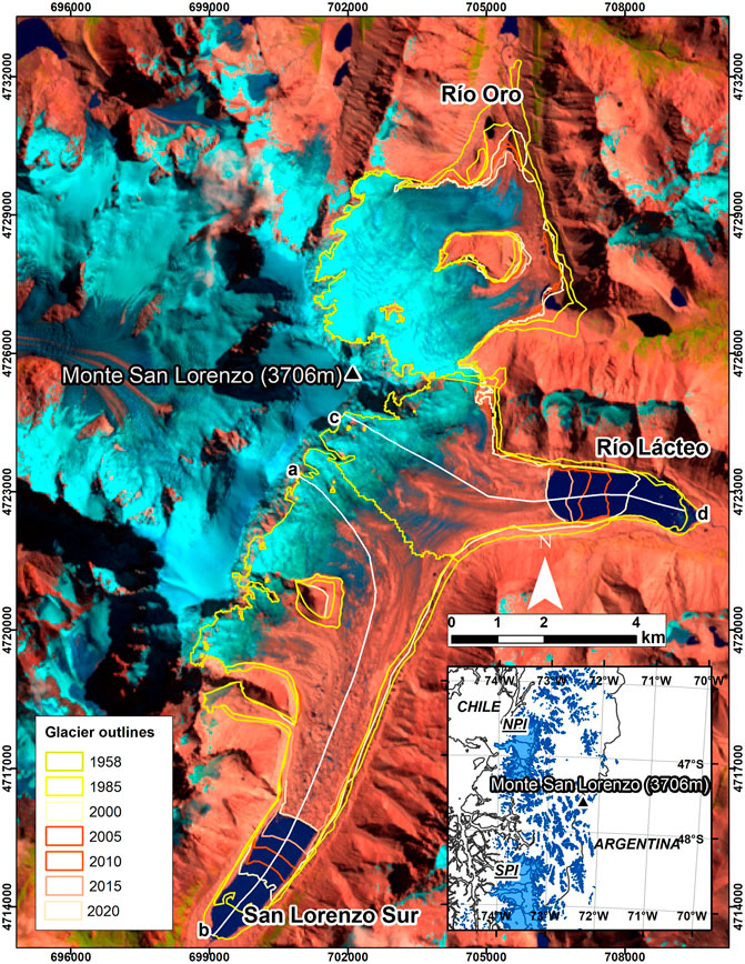
FIGURE 1. View of the investigated glaciers in the Monte San Lorenzo and location of the study area in relation to the Northern (NPI) and Southern Patagonian Icefields (SPI). Coordinates are UTM WGS84 Zone 18 S. a–d are the surface velocity profiles detailed in Figure 5.

The Monte San Lorenzo area is presently well-researched in terms of the number and area of glaciers, the hypsometrical distribution of debris-covered and debris-free ice, and the rates of glacier recession (1% a⁻¹ in the last ∼3.5 decades; Falaschi et al., 2013). The three glaciers investigated in this study have thinned at considerable rates since the mid- 20th century in spite of the debris cover, particularly in comparison to nearby debris-free glaciers (Falaschi et al., 2017). A strong link between climate variability (added to the influence of calving dynamics on proglacial lakes) and glacier mass loss has been made (Falaschi et al., 2019). Sagredo et al. (2017) estimated (>1,600 m asl) paleo- and modern ELAs for the Tranquilo glacier in the northern flank of Monte San Lorenzo. There is currently, however, no detailed information about how climate change and altitudinal shifts of ELAs with time have promoted the development of debris layers and how the inception of feedback mechanisms between glacier dynamics (e.g. glacier flow velocity), morphological features (ice cliffs, supraglacial ponds) and glacier geometry have affected the evolution of these particular glaciers.

Glacier inventories in Southern Patagonia have shown that the surface of both outlet and mountain glaciers is mostly free of debris, and that the amount of debris-covered ice is usually marginal in comparison (e.g. Glasser and Jansson, 2008; Paul and Mölg, 2014; Masiokas et al., 2015; Glasser et al., 2016). In some specific areas of extremely abrupt relief, high valley walls and lateral moraines can be the source of larger quantities of supraglacial debris, and extensive debris layers and debris-covered glaciers can exist, such as in the Monte San Lorenzo massif. Río Lácteo and San Lorenzo Sur are valley glaciers lying at the very bottom of Monte San Lorenzo’s >2,000 m nearly vertical East face, have lake-terminating fronts and noticeable debris layers in an otherwise largely debris-free glacier inventory in the area (Falaschi et al., 2013). On the other hand, Río Oro has a minor proportion of debris-covered area compared to Río Lácteo and San Lorenzo Sur, and its only partially calving-type.

Probably because of their relevance as contributors to sea-level rise (Dussaillant et al., 2019), much scientific research upon the impact of climate change on glaciers has been focused in the nearby Patagonian Icefields. Numerical Modeling and mapping of ELAs and Accumulation Area Ratios (AAR) from remote-sensed data has been carried out to test the mass balance sensitivity of glaciers (Barcaza et al., 2009; De Angelis, 2014). In the periphery of the Patagonian Icefields, however, there are still a vast number of smaller mountain glaciers that can provide complementary information for refining our understanding of overall glacier dynamics and glacier-climate interactions.

Data and Methods

For this study we used 1) a set of orthophotos derived from archival aerial images, 2) medium resolution satellite imagery (Landsat 5, 7, 8, SPOT 5, Sentinel 2) available from various archives and 3) high spatial resolution satellite imagery (Pléiades) available from Google Earth. Unfortunately, during the commercial phase of Landsat, Thematic Mapper (TM) data for Southern Patagonia between 1984 and 1997 was not acquired beyond very few local requests (Goward et al., 2006). In general, these scenes are not suitable for glacier mapping (due to cloud cover or seasonal snow), and thus this period had to be omitted from the analysis (except for the 1985–1986 interval). The main characteristics of the implemented imagery (including spatial resolution, usage of each scene/photo is described in Supplementary Table S2, whereas Supplementary Table S3 shows the time span covered on each of the specific analyses caried out in this study.

Glacier-specific geodetic mass balance values for the 1958–2018 period, as well as length and area changes for the investigated glaciers are available from Falaschi et al. (2019). These data are essential for shedding further light into the interaction of debris covers and the dynamic evolution of glaciers, and therefore incorporated to the discussion sections.

Mapping of the Debris-Covered Ice Extent

Glacier outlines for the years 1958, 1981, 2000, 2012, and 2018 were retrieved from Falaschi et al. (2019). For all the remaining survey years, we modified the glacier outlines by visual interpretation of Landsat scenes. In the 1958 and 1981 orthophotos produced by Falaschi et al. (2019), we mapped the extent of debris layers on each individual glacier by on-screen manual digitization. We considered only areas with a fairly continuous debris cover extent, discarding this way small debris patches and very thin debris covered areas. Excluding now the years 1958 and 1981, debris-covered ice area for each survey year was obtained by calculating the debris-free area on the corresponding Landsat scene (from which the glacier outline had been previously generated), using a thresholded ratio image of the NIR/SWIR band (Paul et al., 2015), and substracting the debris free mask from the total glacier area.

So far, a number of (semi) automatic methods for identifying and mapping of debris-covered ice have been proposed (e.g. Shukla et al., 2010; Racoviteanu and Williams, 2012; Rastner et al., 2014). These approaches, which combine multi-spectral and terrain analyses, are a good approximation and reduce processing time, but ultimately require additional manual corrections to produce the final glacier outlines. Paul et al. (2004) stated that after manual editing, the accuracy of the debris-covered glacier outlines can be equal to pixel resolution. We have thus calculated the uncertainty in debris-covered area by implementing ±1 pixel buffers around the debris-covered ice area. Conservatively, the uncertainty in the debris-covered area change between 1958 and 2020 (σ_dc.tot) was calculated by quadratically summing the uncertainties of the initial (σ_dc.i) and final (σ_dc.f) debris-covered areas:

${\sigma }_{\text{dc}\text{.tot}}=\sqrt{{\sigma }_{\text{dc}\text{.i}}^2+{\sigma }_{\text{dc}\text{.f}}^2}(1)$

Glacier Surface Velocity

Because glaciers are constantly adjusting and redistributing ice mass in an effort to reach an equilibrium state, ice surface velocity is frequently used as an indicator of glacier mass balance conditions and dynamic state (Wilson et al., 2016b). This relationship assumes that during positive mass balance conditions ice surface velocities increase due to increased ice deformation and vice versa. Here we used Landsat 5–7, ASTER, SPOT 5, and Sentinel-2 images to automatically obtain velocity field maps of the three investigated glaciers for the 1985–1986 and 2000–2020 periods. The 1958–1981 and 1981–1985 observation periods were omitted from this analysis due to the lack of corresponding surface features in the imagery used (preventing the use of manual feature tracking techniques e.g. Mölg et al., 2019).

The optical satellite imagery was processed in the CIAS feature-tracking algorithm (Kääb and Vollmer, 2000). This algorithm calculates sub-pixel displacement and direction magnitudes by first coregistering a master (t1 or initial epoch) and slave (t2 or final epoch) images and then comparing the coordinates of the highest correlation pixel block in a search window of the slave image with those of the master pixel block. Given the relatively low speed flow expected for the Río Lácteo and San Lorenzo Sur glaciers, a time separation of ∼1 year between the initial and final scenes was required to detect significant glacier flow that would surpass the total uncertainty in surface velocity (see below). For survey intervals where the initial and final images differed in spatial resolution (e.g. Landsat TM and Landsat ETM+), the highest resolution were resampled to the coarser one before coregistration (Wilson et al., 2016b). Once the CIAS output displacement vectors were generated, a correlation threshold between the initial and final pixel block of r > 0.4 was used to remove abnormal velocities. The resultant displacement points were upscaled to annual velocities and converted to raster grids. The final output cell size of the velocity maps was 30 × 30 and 45 × 45 m for Landsat ETM+ and Landsat TM pairs, respectively. Due to the lack of identifiable features on the debris-free ice, only some portions of the debris-covered tongue of Río Oro can be derived and velocity variations along longitudinal profiles cannot be entirely identified. This prevented a full comparison between the velocity map of Río Oro and the neighboring Río Lácteo and San Lorenzo Sur.

The total uncertainty associated with each glacier velocity map σv_tot was calculated for a given time interval as the quadratic sum of the systematic (σv_sys) and random (σv_rand) uncertainties, following the laws of error propagation (Berthier et al., 2003):

$\sigma {\text{v}}_{\text{tot}}=\sqrt{\sigma {\text{v}}_{\text{sys}}^2+\sigma {\text{v}}_{\text{rand}}^2}(2)$

The systematic uncertainty σv_sys depends on the performance quality of the image cross-correlation algorithm and typically, a ±2 pixel accuracy is expected for Landsat scenes:

$\sigma {\text{v}}_{\text{sys}}=\frac{2R}{\Delta t}(3)$

where R is the pixel size and Δt the time separation between the initial and final epochs in days. In turn, the random uncertainty σv_rand is measured over stable terrain (off-glacier), in a buffer area around each individual glacier outline minus shadow areas and overlay steep terrain (>25°).

Identification of Ice-Cliffs and Supraglacial Ponds

Mapping of ice exposures (cliffs and supraglacial drainage channels, Supplementary Figure S1) has been carried out in different studies by means of object-oriented and principal components analyses in satellite and aerial imagery (Racoviteanu and Williams, 2012; Mölg et al., 2019), slope thresholding of high-resolution elevation data (Herreid and Pellicciotti, 2018), linear spectral unmixing approaches (Kneib et al., 2021), and of course, by on-screen digitizing of high resolution satellite imagery (Watson et al., 2017; Steiner et al., 2019). For the sake of simplicity, here we mapped ice cliffs and ponds by on screen digitization. We also mapped exposed ice in supraglacial drainage channels, but excluded heavily crevassed areas. The terminal portion of the San Lorenzo Sur glacier was not fully covered in the 2011 imagery available on Google Earth.

Since the ice cliffs and supraglacial ponds located on the glaciers investigated here are relatively small in size, only the highest resolution (<1 m) imagery available from our dataset was used (see Supplementary Table S2). The Minimum Mapping Unit (MMU) is the smallest sized object that determines whether an object can be identified and mapped in remotely sensed imagery, and needs to be four contiguous pixels in size. In this way, we mapped ice cliffs ≥4 m², which is the MMU of our lowest resolution data (aerial photos, 1 m resolution). On the other hand, intra-annual variations in both number and area of supraglacial ponds between seasons has shown to be significant (Steiner et al., 2019). We have minimized this potential bias by mapping ponds on images acquired from very late spring (December 10, 2009) to mid-summer (February 22, 2018).

The overall accuracy of manual mapping of ice cliffs is dependent on several sources of uncertainty, including the spatial resolution and quality of the utilized imagery (optical contrast, shadows), and the user’s inherent mapping subjectivity when identifying an ice cliff and its characteristics. Some studies aiming to map ice cliff geometry exhaustively (including information regarding slope, aspect, slope area) have carried out in-depth delineation uncertainty assessments (Steiner et al., 2019), by checking ice cliff outlines and omissions made by multiple users and slope analyses derived from high resolution DEMs. Whilst such a thorough quality evaluation was not considered here, three independent operators inspected visually all individual ice-cliffs, whilst we also carried out a multiple user digitization of 50 randomly selected cliffs on each scene (Watson et al., 2017). Results of the round-robin digitizations are provided in Supplementary Table S4 and Supplementary Figure S2. We observed two main sources of uncertainties in ice-cliff mapping. One source is related to inherent imagery properties, not necessarily related to spatial resolution, but rather image illumination conditions and contrast (aerial photos were the least adequate in this regard). The second source relates to ice-cliff specifics such as complexity or branchiness, preservation/degradation state and debris layer thickness on ice exposures.

In addition to the ice cliff inventory, we also investigated ice cliff evolution in terms of changes in mean size and total area, and the altitudinal distribution of ice cliffs through time. This was done by calculating the relative proportion of ice-cliff area per 50 m elevation band across each glaciers’ debris-covered surface.

Snowline Altitude and Climate Records

Mapping of the Transient Snowline Altitude

We mapped the elevation of the transient snow line (SLA) and Snow Cover Ratio (SCR, defined as the snow-covered area with respect to the total glacier area) for Río Oro, Río Lácteo, and San Lorenzo Sur glaciers. To infer possible ELA changes with time for the three surveyed glaciers, we relied on the assertion that the Snow Line Altitude at the end of the hydrological year provides an effective proxy of the equilibrium line in temperate glaciers (Rabatel et al., 2008 and references therein) for that specific year. Because differences between the theoretical annual ELA and the snowline may exist at the end of summer (due to mass additions or losses e.g. superimposed ice or atypical length of the ablation period), the term end of summer snowline has been coined in the Southern Hemisphere (Clare et al., 2002).

The main limitations for deriving end of summer snowlines lies in that suitable satellite imagery for snow mapping on glaciers (no cloud cover or fresh snow on glacier surfaces), DEMs and glacier outlines when dealing with a long time series are not always available for each individual year. To minimize this impact, we implemented a prototype version of the Automatic Snow Mapping on Glaciers (ASMAG) tool (Rastner et al., 2019), running now on the Google Earth Engine (GEE) platform. The algorithm currently maps SCR from Landsat and Sentinel 2 scenes, after converting digital numbers to top of atmosphere reflectance. The histogram approach of Bippus (2011) is then used within a single glacier mask to distinguish snow from ice by implementing an automatic threshold based on the Otsu (1979) thresholding algorithm to the Near Infrared (NIR) band (Rastner et al., 2019). After comparing the automatic derived snow cover area with the manual digitized ones, it became obvious that the ASMAG approach leads to systematically lower values compared to the manual derived ones (mapped on RGB true color compositions). We attribute this to the still missing topographic correction procedure not yet implemented in the GEE procedure so that we used this prototype in this study only for a straightforward selection of the satellite scene with the highest SLA for each single survey year. After knowing all the automatic derived acquisition dates with the highest SLAs (termed “SLAs” hereafter) for each period (ranging between February 1 and April 10), we manually digitized the snow cover area to retrieve SLAs based on three DEMs (SRTM-X, ALOS PALSAR and Pléiades) for three different time periods (2000–2009, 2010–2017, and 2018–2020).

End of Summer Snowline Altitude and Climate

Here we investigate the influence of temperature and precipitation on the end of summer snowline elevations (and consequently ELAs) on Río Oro, Río Lácteo, and San Lorenzo Sur glaciers. For the 2000–2020 period, we performed correlation analyses between mapped snowlines and monthly, annual and seasonal (summer, autumn, winter and spring) temperatures of the Balmaceda meteorological station (45.912°S, 71.694°W, 517 m a.s.l.), retrieved from the GISS-NASA portal. A similar analysis was carried out, relating monthly precipitations for the December and January months prior to the February-March snowline mapping. Results are presented as the individual temperature and precipitation influence on both glacier-specific and glacier-averaged SLAs, as well as the joint temperature and precipitation influence, again at both glacier-specific and glacier-averaged scale. For all statistical analyses, we used a confidence interval of 95%.

Results

Debris-Covered Area Evolution

Among the three sampled glaciers, the total glacier area was 60.6 ± 1 km² in 1958 and 46 ± 0.8 km² in 2020. This represents an area reduction of 14.6 km² (∼0.25 km² per year) (Figure 1). Individually, Río Lácteo glacier had the largest (relative) area loss (29.2%; 4.7 km²), followed by San Lorenzo Sur (22.8%; 5.7 km²) and Río Oro (22%; 4.3 km²).

The oldest dataset available for the Monte San Lorenzo region, from which the extent of the debris-covered ice can be quantified are the 1958 orthophotos. At this time, 48 ± 0.4% (12 ± 0.1 km²), 32 ± 0.6% (5.2 ± 0.1 km²) and 15 ± 0.5% (3 ± 0.1 km²) of San Lorenzo Sur, Río Lácteo, and Río Oro area (20.2 ± 0.3 km² 40 ± 0.6% overall) respectively, were debris-covered. Later imagery reveals (Figure 2) that the debris-covered extent has expanded up-glacier to higher elevations on all three glaciers. By 2020, the debris cover area percentage has risen to 71 ± 6.7% on San Lorenzo Sur, 54 ± 6% on Río Lácteo and 19 ± 4.9% on Río Oro (50 ± 6.7% in total).

FIGURE 2

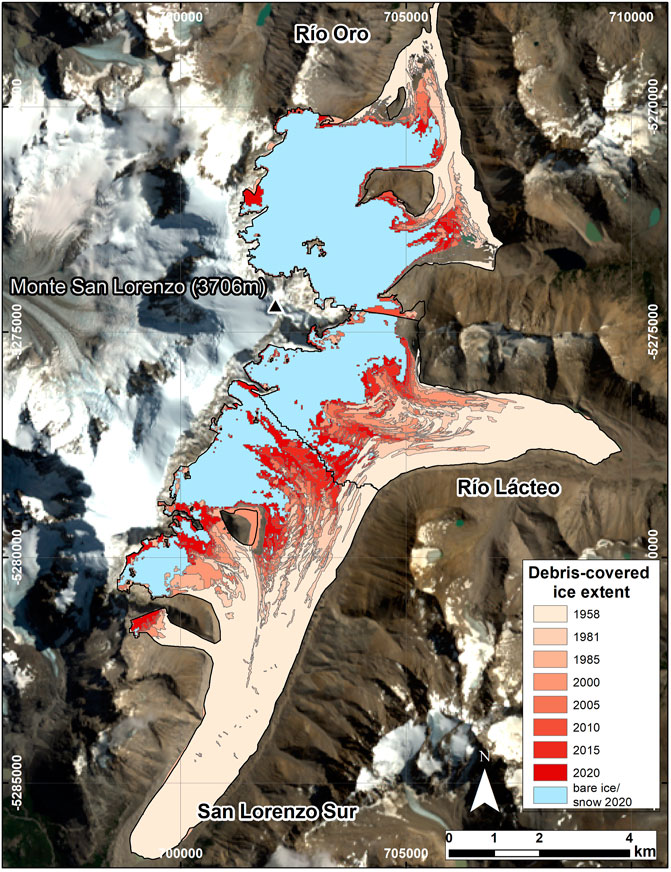
FIGURE 2. Evolution of the debris-covered ice extent through time and the remaining bare ice and snow. Background image is a 2020 Landsat 8 RGB 654 false color composition.

Linear fits of the percentage of debris-covered area as a function of time revealed a trend of progressively higher percentages of debris-covered area on Río Lácteo (0.2% a⁻¹) and San Lorenzo Sur (0.24% a⁻¹) glaciers up to the year 2020, whereas there is no clear trend for Río Oro (Figure 3). In principle, expansion of proglacial lakes affecting the lowest part of the glaciers should lead to a smaller proportion of debris-covered glacier area, yet our results show that yearly debris input has compensated the debris-cover area losses through calving. Indeed, if the yearly debris-covered area is divided by the initial 1958 total glacier area, the debris-covered area increase rates rise to 0.38% a⁻¹ (San Lorenzo Sur), 0.48% a⁻¹ (Río Lácteo), and 0.33% a⁻¹ for Río Oro. The regression analysis of debris-covered area with time for these later cases revealed statistically significant (p < 10^–3 for all glaciers), very high r values of 0.86 (Río Oro), 0.91 (Río Lácteo) and 0.96 (San Lorenzo Sur) at the 95% confidence level.

FIGURE 3

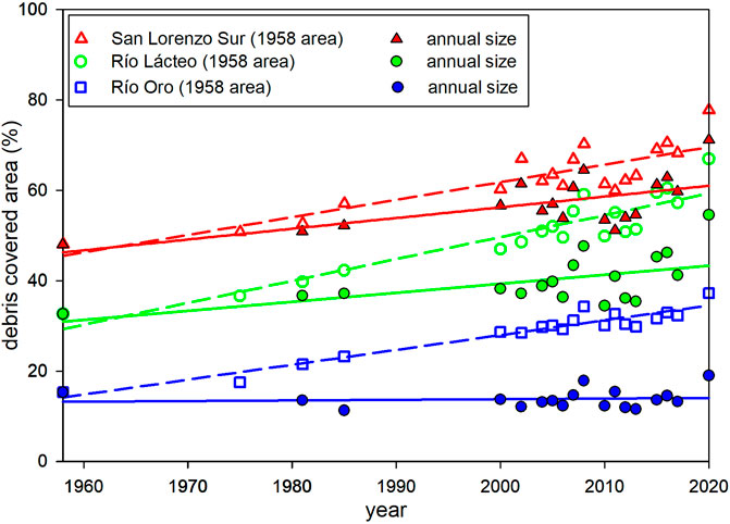
FIGURE 3. Scatter plot showing the debris cover increase through time. The color-void (and regression dashed line) symbols show the percentual increase of debris-covered ice area considering the initial 1958 glacier area, and the color-filled symbols (regression solid lines) depicts the increase taking the actual glacier size for each survey year into account.

Concomitantly to the increase in debris-cover area, debris layers have progressively occupied higher elevations on glacier surfaces as well. Between 1958 and 2020, sporadic debris has appeared on accumulation areas, shifting the maximum elevation of debris-covered ice from 1,570 to 3,240 m on Río Oro, 1,515–2,840 m on Río Lácteo, and 1,700–2,840 m on San Lorenzo Sur. Considering the glacier thinning that has taken place during this time interval (Falaschi et al., 2019), mean elevation of the debris covered ice has increased ∼240 m (1,130–1,370 m) on Río Oro, ∼130 m (1,320–1,450 m) on Río Lácteo, and ∼160 m (1,280–1,440 m) on San Lorenzo Sur.

Regarding the thickness of the debris layer on the glaciers investigated, we did not undertake systematic in situ surveys, nor did we estimate it from remote sensing data. Field observations on ice exposures (crevasses, ice cliffs) of Río Lácteo (Supplementary Figure S1), however, revealed a rough estimate of debris thickness between 1 and 2 m in proximity of the glacier terminus. In the lateral margins, boulders up to ∼3 m in diameter are frequent, these possibly resulting from the degradation of the lateral moraines. Thickness of the debris layer progressively decreases in the upward direction and in the uppermost part of the debris-covered tongue, close to the debris-free ice, the debris layer is pebbly in grain size, a few centimeters thick and interspersed with ∼10 cm blocks.

Glacier Velocities

Glacier velocity profiles and maps and were produced for Río Lácteo and San Lorenzo Sur glaciers for the 1985–1986 and 2000–2020 periods (Figures 1, 4, 5). In terms of spatial distribution, the highest velocities for both glaciers were found at the steep icefalls located just below the vertical rock wall of Monte San Lorenzo’s East Face (∼90 ± 33 and ∼75 ± 55 ma⁻¹) for Río Lácteo and San Lorenzo Sur, respectively). In the case of San Lorenzo Sur, velocities steadily decrease from these icefalls toward the terminus, where the extremely low velocities (<18 ± 29 m a⁻¹) indicate that the glacier terminus is practically stagnant. Aside from the icefall area, the velocity maps for Río Lácteo show higher velocities around the central flow line and a flow speed increase toward the calving front which is visible between 2012–2014 and 2018–2020 (maximum velocity of ∼51 ± 34 m a⁻¹ in 2020) (Figures 4, 5).

FIGURE 4

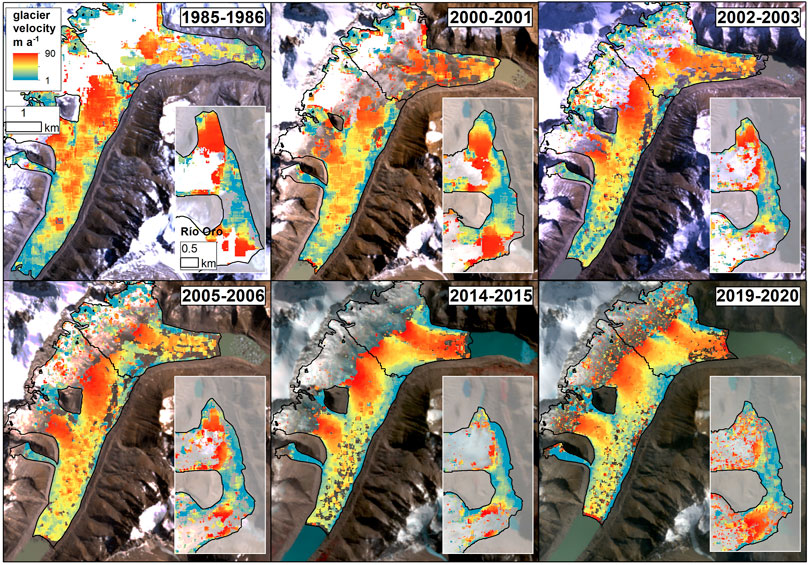
FIGURE 4. Examples of glacier flow velocity maps selected for six survey periods.

FIGURE 5

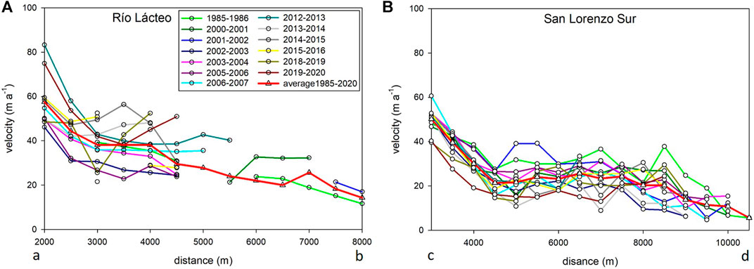
FIGURE 5. Glacier flow velocities for longitudinal profiles on Río Lácteo (A) and San Lorenzo Sur (B).

Overall, we found that the spatio-temporal patterns and magnitudes of ice flows at both glaciers were fairly constant during the survey period (1985–2020). For both glaciers, average velocities only fluctuated within a narrow range of ±36.5 m a⁻¹ along the whole length of the glaciers, and no significant trends of progressive velocity decrease were detected for the longer 1985–2020 time span (Figure 5). Short-term variations were detected during sub-periods (e.g. speed-ups between the years 2001 and 2007, deceleration between 2015 and 2020), however, these changes were small in magnitude and within the displacement error rate calculated for nearby stable terrain.

Inventory and Area Changes of Ice Cliffs and Supraglacial Ponds

We found that the number of ice cliffs at the individual glacier scale increased considerably during the observation period, with the total count more than doubling between 1958 (639) and 2018 (1,395) (Table 1). This increase, however, amounts only to a relatively small change in the area occupied by ice cliffs (0.65 ± 0.07 and 0.78 ± 0.02 km²). In absolute terms, the maximum in total ice cliff area (1.02 km²) occurred in the year 2009. Individually, the percentage of ice-cliff area on debris-covered ice varies strongly between glaciers, from an absolute minimum of 0.3 ± 0.1% on Río Lácteo (1958) to a maximum of 7.6 ± 2% on San Lorenzo Sur (2009). Between 1958 and 2018, the overall percentage of ice-cliff area on debris-covered ice increased only slightly from 3.2 ± 0.3 to 3.8 ± 0.1% (Table 1). Individually, San Lorenzo Sur showed the largest increase in ice cliff area (4.8 ± 0.6–6.1 ± 0.2%).

TABLE 1

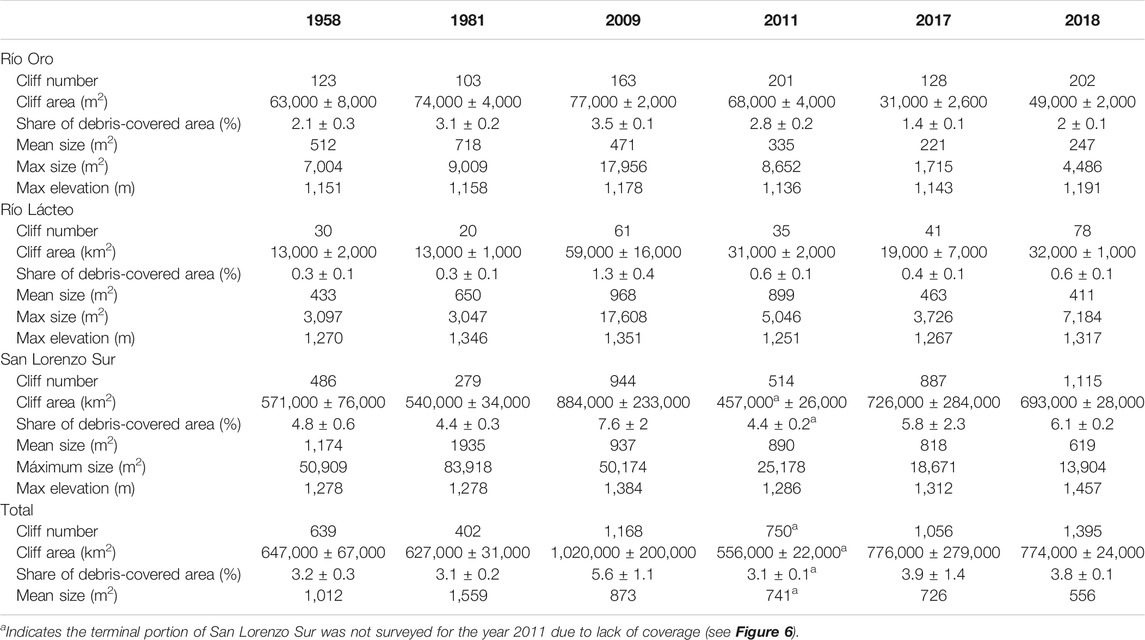
TABLE 1. Glacier-specific main characteristics of ice cliffs.

For all surveyed years, San Lorenzo Sur was found to have the highest concentration of ice cliffs amongst the investigated glaciers, accounting for 75–85 and 85–90% of the total cliff number and area, respectively (Table 1). For this glacier, the total ice-cliff area ranged between ∼0.54 ± 0.06 and ∼0.89 ± 0.23 km², whereas the average area of individual ice-cliffs varied between 670 and 1,900 m². Over time, glacier retreat and proglacial lake expansion removed a number of ice cliffs in the glacier lowest sections, though we still observed a number and area increase of ice cliffs. This possibly means that the relative number increase would be much more if the glaciers had land-terminating tongues. Interestingly, we also found that the maximum and mean area of ice cliffs decreased with time except for the year 1981, when the largest identified ice cliff was 83,918 m² on San Lorenzo Sur and caused an anomalously high mean size.

Another aspect of ice-cliff evolution is the increasing altitudinal range at which ice cliffs occur (Table 1). Overall, the upper limit of this range has shifted toward higher altitudes on all three glaciers. For Río Oro (1,140–1,190 m) and Río Lácteo (1,270–1,320 m) glaciers, the shift was 40–50 m. The altitudinal shift of ice cliffs is better exemplified at San Lorenzo Sur glacier, where the increase is ∼180 m (1,280–1,480 m). When calculating the percentage share of ice-cliffs within debris-covered areas by elevation (considering 50 m elevation bands), we found that ice-cliffs began to form above 1,250 m at least from the year 2009 onwards, and that ice-cliff area below 1,150 m (the lowermost portion of the glacier tongue) decreased after the same year (Figure 6), probably as a consequence of fast glacier area removal by calving processes.

FIGURE 6

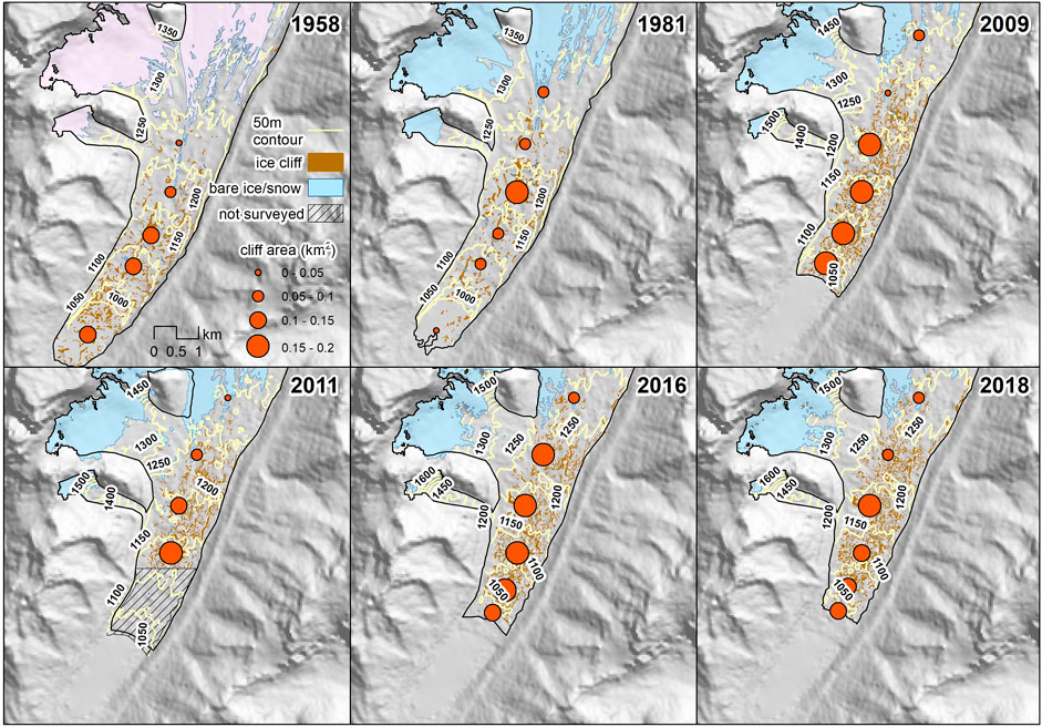
FIGURE 6. Ice cliff and pond distribution and temporal evolution in the San Lorenzo Sur glacier.

In comparison to ice-cliffs, the total area and number of supraglacial ponds was found to be consistently smaller, representing merely 0.3% of the total debris-covered area at all times among the three sampled glaciers. The total number and area of supraglacial ponds was shown to be highly variable on all three glaciers across time, with San Lorenzo Sur again hosting the highest concentration (∼70–90% in number). The total pond area on this glacier varied between 0.04 and 0.06 km², whereas the mean size ranged between 350 and 780 m². Except for the two initial survey years (1958 and 1981), more than 50% of supraglacial ponds were associated with an ice-cliff (Table 2). For the most recent 2018 pond inventory, 38% of the ponds were situated on debris-covered ice surfaces with no relation to a cliff, 36% occur at the bottom of longitudinal or lateral cliffs, 13% are contained within a circular cliff, and a further 13% are associated with complex cliffs.

TABLE 2

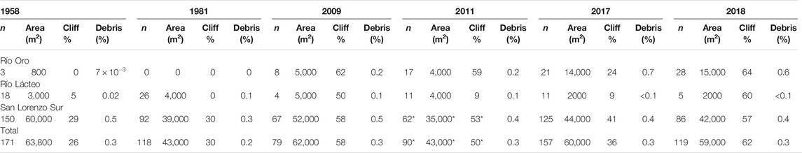
TABLE 2. Number (n) and area of supraglacial ponds through time. The cliff % column stands for the percentage of ponds that are in contact with ice cliffs, and the debris (%) column refers to the debris-covered area share of the supraglacial ponds.

Changes in Snow Cover Ratio and Snow Line Altitude

Snow Cover Ratios and Snow Line Altitudes were calculated for Río Oro, Río Lácteo and San Lorenzo Sur glaciers. In general, Río Oro has always the greatest SCR values (mean = 0.44), whereas the (average) minimum SCR of Río Lácteo and San Lorenzo Sur are 0.23 and 0.16 respectively (Figure 7). Data reveal also that when the minimum SCR values for each survey year are considered, SCR appears to have diminished with time on all three glaciers. Linear fits for the SCR scatter data suggest moderate to high correlation (statistically significant with α = 0.05) with time for Río Lácteo (r = 0.6; p = 0.007), Río Oro (r = 0.7; p = 0.001) and San Lorenzo Sur (0.76; p = 2 × 10⁻⁴). The maximum SLA varied strongly on a yearly basis on all glaciers, with altitudinal differences between maximum and minimum values of up to ∼800 m on Río Oro and ∼600 m on Río Lácteo and ∼500 m San Lorenzo Sur. For the full study period, the averaged maximum SLA was 1905 ± 100 m (Río Oro), 1720 ± 85 m (Río Lácteo) and 1815 ± 165 m (San Lorenzo Sur).

FIGURE 7

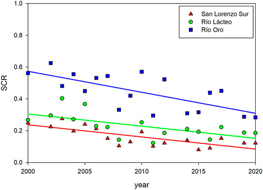
FIGURE 7. Scatter plot showing Snow Cover Ratios (SCR) for the 2000–2020 period. Note the absence of data for years 2013 and 2018.

Relationships Between Late-Summer Snowline and Climate Variables

At the monthly scale, March temperature is significantly related to SLAs (Figures 8, 9; Table 3). This is not surprising, since most of5 the snow line determinations were based on satellite images collected during March. Although the correlation coefficients between March temperature and SLAs are significant for all three glaciers, the relationship is stronger when considering the glacier-averaged SLA in all three areas (r = 0.64, p < 0.01; see Figure 8A). Based on this result, we show that March temperature explains about 37% of the total variance of SLA in the 2000–2020 interval. The annual temperature, from December of the previous year to November preceding the SLA determination, is also significantly associated, although weaker (r = 0.58), to the SLA, indicating that SLA variations are also influenced by snowpack accumulation during the previous year.

TABLE 3

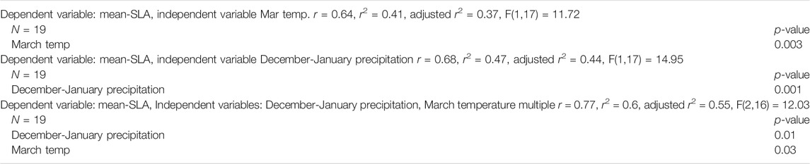
TABLE 3. Regression summaries for mean snowline altitudes (mean-SLA) using March temperature, December-January precipitation, and both variables as predictors.

FIGURE 8

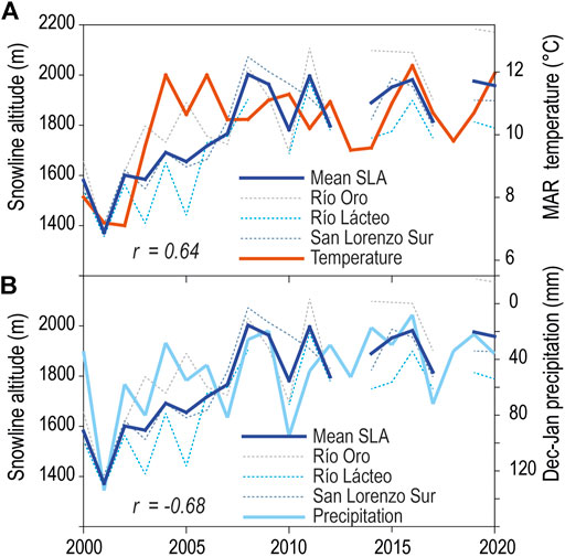
FIGURE 8. Relationships between variations in yearly snowline altitude, March temperature (A) and accumulated December-January precipitation (B).

FIGURE 9

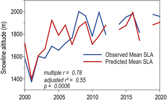
FIGURE 9. Observed (blue) and predicted (red) snowline altitudes as a function of March temperatures and December-January precipitation.

December-January precipitation is the seasonal arrangement most significant related to SLA. Similar to temperature, the relationships improve when the comparison between December and January precipitation is based on the glacier-averaged SLAs (r = 0.68; see Figure 8B). The percentage of total variance in SLAs changes explained by December-January precipitation over the interval 2000–2020 is somewhat higher (R² around 44%) than that accounted by temperature.

The joint use of March temperature and December-January precipitation from Balmaceda as predictors of the SLAs at Mount San Lorenzo in a regression analysis shows that these climatic variables can explain more than 50% of the total variance of the glacier-averaged SLAs during the period 2000–2020 (adjusted r² = 55%, F(2,16) = 12.031 p < 0.00065; Figure 8 and Table 3). However, we noted that each climatic variable has a distinctive impact on each of the glaciers (Table 4). For the Río Oro glacier, the total variance explained by both climatic variables is high (adjusted r² = 50%), but only December-January precipitation is a significant (p = 0.009) predictor for SLA variations in this glacier. For the Río Lácteo glacier, the explained SLA variance remains significant (adjusted r² = 41%) but none of the predictors are statistically significant at 95% confidence level (p = 0.054 and p = 0.085 for December-January precipitation and March temperature, respectively). Finally, the SLA variance explained for the San Lorenzo Sur glacier is adjusted r² = 40%, with March temperature being statistically significant (p = 0.033) as a regression predictor (Table 5).

TABLE 4

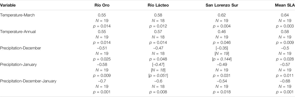
TABLE 4. Correlation matrix between snowline altitude, temperature (March and Annual [December-November] and precipitation (December, January, joint December and January) on Balmaceda weather station. Non-significant r values at p < 0.05 are marked in [Italics].

TABLE 5

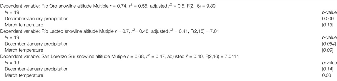
TABLE 5. Regression summaries for snowline altitudes at individual glaciers using March temperature and December-January precipitation as predictors. Non-significant r values at p < 0.05 are marked in [Italics].

Discussion

Increase in Debris-Covered Area

Overall, the total extent of debris-covered ice area for the three glaciers investigated has increased from 40 ± 0.6% to 50 ± 6.7% from 1958 to 2020. Because glacier recession in this study area is significant due to calving in proglacial lakes (particularly in the cases of Río Lácteo and San Lorenzo Sur), each year a large amount of debris-covered ice is lost (Falaschi et al., 2017). The above estimate of debris-covered area increase represents thus a minimum value of the potential debris-covered ice area increase. To give a better idea of the above, it can be said that if the initial 1958 glacier area is kept for all calculations (i.e., omitting all area losses since 1958 due to calving), the increase would be from 40 to 56%. Throughout the study period, the total debris-covered ice area has increased a steady rate, and we were unable to detect any short-term migration of the upper boundary of the debris layer toward lower elevation.

Most debris input probably originates from the headwalls of each glacier, especially the East Face of Monte San Lorenzo, where the accumulation areas of the investigated glaciers are located. Although lateral moraine degradation is relevant on the investigated glaciers (Falaschi et al., 2019), we infer from the field visit to Río Lácteo glacier that they contribute merely to the glacier margins in the form of large boulders. Incidentally, van Woerkom et al. (2019) also showed that debris supply from lateral moraines alone cannot explain thick and continuous debris layers on debris-covered glacier surfaces. On the sampled glaciers here, no large rock avalanches were detected, which would rapidly add to the debris-covered area (see e.g. Berthier and Brun, 2019).

In the nearby Northern Patagonian Icefield, Glasser et al. (2016) found an increase in the number of debris-covered glaciers and a relative increase of ∼4% in debris-covered ice area between 1987 and 2015. Given the much larger size of the outlet glaciers investigated by Glasser et al. (2016) compared to the Monte San Lorenzo glaciers, this seemingly minor relative increase of ∼4% is naturally much larger in terms of the total debris-covered area (139 vs. ∼3 km² in San Lorenzo). Our findings nevertheless confirm that the trend of increasing debris-covered area is taking place not only in the large ice masses of the Patagonian Icefields, but also in the smaller mountain glaciers in their periphery. In recent decades, expansion of debris-covered ice areas has also been observed in the Himalayas, Karakorum (Bolch et al., 2008; Bhambri et al., 2011; Kirkbride and Deline, 2013; Xie et al., 2020), Caucasus (Tielidze et al., 2020) and the European Alps (Mölg et al., 2019), mostly at decadal to subdecadal scale.

Interaction Between Flow Velocity, Mass Balance, Proglacial Lakes and Ice Cliff Evolution

The flow velocity time series produced here for Río Lácteo and San Lorenzo Sur glaciers is, despite its relatively shortness, the longest one available for Patagonia beyond the outlet glaciers of the Patagonian Icefields (Mouginot and Rignot, 2015). The unavailability of Landsat TM imagery acquired during the second half of the 1980’s and most of the 1990’s, added to the persistent cloud cover in this region, preclude a longer and high temporal resolution assessment. Whilst some studies have used large boulders visible on old aerial photos to derive isolated and sporadic velocities (e.g. Mölg et al., 2019), this was not possible in our case, as the morphology of the glacier surfaces being observed have transformed greatly between the acquisition of our 1958 and 1981 aerial photographs and the availability of the first satellite images.

A possible explanation for the differences in flow speed evolution between Río Lácteo and San Lorenzo Sur described in Glacier Velocities may be related to the dynamic effect originating at the glacier fronts in response to local lake water depths. Greater proglacial depths enhance calving at the snout of lake-terminating glacier tongues due to increased glacier-lake contact area subjected to subaqueous melt, accelerating flow rates and ice flux toward glacier terminus (Kirkbride and Warren, 1997; Benn et al., 2007). Acceleration of flow rates has been in fact acknowledged at the glacier terminus of several glaciers in the Himalaya (Liu et al., 2020; Pronk et al., 2021). The deceleration of San Lorenzo Sur could hence be linked to shallower lake depths, whereas the constant velocities on Río Lácteo (and even slight acceleration of the glacier front in recent years) might be connected to the presence of a deeper proglacial lake and consequently to higher calving rates.

The dynamic thinning described above is highly relevant for understanding glacier dynamics, since it has shown to exacerbate glacier retreat and thinning rates of freshwater calving glaciers compared to land-terminating ones (King et al., 2018; King et al., 2019). Ice velocities close to the front of Río Oro (small panels in Figure 4) are similar to the maximum values found at Río Lácteo and San Lorenzo Sur (∼90 m a⁻¹), though we interpret them as a result of a higher local slope and not a dynamic acceleration due to the presence of a proglacial lake. Falaschi et al. (2019) found a strong relation between higher rates of proglacial lake expansion and increased mass losses. In particular, the 1958–2018 thinning rates of the lake-terminating Río Lacteo and San Lorenzo Sur (1.87 and 1.94 m a⁻¹, respectively) appear to be much stronger than the land-terminating Río Oro (0.92 m a⁻¹).

When comparing average surface velocities along longitudinal profiles on Río Lácteo and San Lorenzo Sur in relation to their geodetic mass balance (as retrieved from Falaschi et al. (2019)), however, we did not find a clear correlation between mass balance and glacier flow rates. The velocity of Río Lácteo did not change significantly between the 2000–2007 and 2012–2018 periods (∼33 m a⁻¹ for both time intervals), whereas mass balance values shifted toward more negative conditions from −1.74 ± 0.05 to −2.09 ± 0.15 m w.e. a⁻¹ for the 2000–2012 and 2012–2018 periods, respectively. Additionally, surface ice flow at San Lorenzo Sur diminished only slightly (∼28–25 m a⁻¹) between 2000–2007 and 2012–2018, whilst mass balance conditions at San Lorenzo Sur remained almost equal (−1.61 ± 0.03 and −1.71 ± 0.16 m w.e. a⁻¹ for 2000–2012 and 2012–2018).

Despite the above limitations in establishing a clear relation between flow speed and thinning rates, it can be argued that the overall mass balance of Río Lácteo and San Lorenzo Sur glaciers is primarily driven by climate variability and calving processes. Indeed, thinning rates increase at lower elevations at all of the investigated glaciers (Falaschi et al., 2019) in spite of the increase in debris layer thickness observed during field trips. Naturally, however, some spatial heterogeneity in the thinning patterns exist due to local variations in debris thickness, which is in turn partly linked to the occurrence of ice cliffs. To quantify the possible influence of ice cliffs on mass balance, we generated buffer zones of 35 m around the mapped ice cliffs (see Mölg et al., 2019) for three time intervals of geodetic mass balance studied in Falaschi et al. (2019). Also included within these buffer areas were supraglacial ponds, as they are closely related to ice cliffs (Watson et al., 2017; Steiner et al., 2019) and actually appear to contribute to their formation. The mean elevation change (dh/dt) in meters per year for the elevation grid cells that correspond to the buffered areas (including actual ice cliffs and ponds) effectively shows higher thinning rates compared to the debris-covered portions that are not affected by ice cliffs/ponds on nearly all glaciers and evaluated time periods (Table 6). This signal of increased ablation at ice cliff location might be even attenuated here, since a given ice cliff might have disappeared or migrated downglacier within each surveyed time interval. In addition, DEM differencing using 30–40 m resolution DEMs might be too coarse for the relatively small ice cliffs. High contribution to glacier ablation from ice cliffs (though seasonally variable) has also been acknowledged on several other debris-covered glacier sites like the Himalayas (e.g. Brun et al., 2016; Buri et al., 2021).

TABLE 6

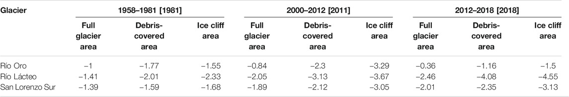
TABLE 6. Elevation changes (m a⁻¹) for full glacier, debris-covered ice and ice cliff areas. The values in bracket for each study period indicate the year in which the ice cliff mapping was carried out.

Another aspect of glacier velocity in relation to the occurrence of glacier surface features (cliffs and ponds) was brought out by Mölg et al. (2019) for the Zmuttgletscher in the Swiss Alps. These authors showed that time intervals of relatively high flow speeds hampered the emergence of ice cliffs, and concomitantly shifted the upper boundary of debris-covered area downglacier. In principle, our results for the investigated glaciers in Monte San Lorenzo agree with this assertion, since we also found a continuous increase in the debris-covered ice area and a steady shift of the upper altitudinal limit of the ice cliff area toward higher elevations during the study period. Average slopes on Río Lácteo and San Lorenzo, as retrieved from a 1958–2018 multi-sourced DEM time series (see Falaschi et al., 2019), have decreased only very slightly on the debris-covered glacier portions between 1958 and 2018 (9°–8° and 11°–9° respectively). The relatively high slopes can explain the still continually flowing glacier tongues, though velocities might be still low enough to have enabled the growth of ice cliff and supraglacial ponds areas at increasingly higher elevation with time. Watson et al. (2017) and Steiner et al. (2019), however, found no clear link between ice cliff spatial density and glacier surface velocity on debris-covered glaciers in the Everest and Langtang regions in the Himalaya, nor a preferential formation sites of ice cliffs on stagnating tongues. Also, Río Oro (3.4% max), and especially San Lorenzo Sur glacier (7.6% max), have a much higher ice cliff share of the debris-covered ice area compared to e.g. Zmuttgletscher (1.5% max), which flows at similar speed compared to San Lorenzo Sur, or a series of five valley glaciers in the Langtang Himalaya (max 3.8%) whose lowermost tongues are almost stagnant (Steiner et al., 2019). Also, the 16–18% annual survival rate of the ice cliffs in the investigated glaciers (measured for the 2009–2011 and 2017–2018 time intervals) happens to be somewhat higher than for Langtang glacier (9–13% Steiner et al., 2019) despite higher flow velocities.

Influence of Snow Line Altitude/Snow Cover Ratio Variability in Glacier Changes

Our satellite-derived SLAs were highly variable in elevation (various hundreds of meters). This is due to limitations posed by the occasionally unavailable actual late-summer imagery to derive the highest SLA for many survey years (Supplementary Table S2). In fact, there was only a single suitable scene for SLA mapping in many years. Hence, images acquired earlier in the ablation season will provide a lower SLA compared to actual late-summer scenes, as long as no snowstorms hit the mountains later in the ablation season. Facing the same limitations, Barcaza et al. (2009) recorded differences of up to 300 m in satellite-derived ELAs for singe glaciers in the Northern Patagonian Icefield between 1975 and 2003.

With the restrictions imposed by the overall limited satellite imagery availability in mind, we found that SLAs have increased during the 2000–2020 time interval (Figures 8, 9). Increasing SLAs are more evident before the year 2008 than for later years, coinciding with the contemporary temperature and precipitation changes during these earlier years. From 2001 to 2008, December-January monthly precipitation decreases from 120 mm to only 20 mm, whereas there is no clear trend afterward. Likewise, March mean temperature shifts from ∼7°C before 2002 to ∼12°C in 2004 and remained fairly stable since then.

Given that the March air temperature and December-January precipitation can explain more than 50% of the total variance of the glacier-averaged SLAs, a first, preliminary conclusion from Changes in Snow Cover Ratio and Snow Line Altitude is that our mapped glacier-averaged SLAs and their changes through time are fairly representative of the climate variability in the Monte San Lorenzo region. Because in the temperate ice masses of Patagonia superimposed ice is not to be expected (Cuffey and Paterson, 2010), end of summer snowlines are a good approximation of ELAs. Therefore, our findings suggest progressively lower Accumulation Area Ratios (AAR) on the investigated glaciers (Figure 7), which is compatible with glaciers in decidedly disequilibrium state (Bakke and Nesje, 2011). Previously, a paleoclimatic reconstruction by Sagredo et al. (2017) in the nearby Tranquilo glacier (in the northern slope of Monte San Lorenzo), estimated a 130–170 m shift in ELA since the Last Millennium Maximum. Further supportive data to this assertion comes from Glaciar de los Tres, ∼200 km south of San Lorenzo (but still the closest glacier where in-situ measurements are available). Here, glaciological surveys have also shown rapidly increasing ELAs since the late 1990s (WGMS, 2020).

Climate data presented in Falaschi et al. (2019) indicate that there have been clear trends of diminishing annual precipitation and increasing summer air temperatures in the Monte San Lorenzo region, at least since the mid-20th century, promoting rising ELAs in the district. The observed increase in debris-covered area in the sampled glaciers may hence stem not only from the low glacier flow speeds that fail to evacuate debris from the glaciers’ surface, but also from the enhanced emergence of englacial debris at higher elevations up-glacier due to higher SLAs with time. In consequence, climate forcing (by way of changes in SLAs through time) needs to be incorporated as a causing factor in the feedback interactions governing the dynamics of the investigated glaciers.

In regards to changes in SLAs and glacier mass balance, we split the 2000–2020 observation period into two sub-periods (2000–2012 and 2012–2020) to match the geodetic mass balance intervals sampled in Falaschi et al. (2019), and found a shift of time-averaged SLAs toward higher elevations on all three glaciers (∼300 m on Río Oro, ∼120 m on Río Lácteo and ∼100 m on San Lorenzo Sur). In principle, rising SLAs (ELAs) should promote higher thinning and ablation rates, as a now larger portion of the glacier is under melting conditions and the glacier surface is exposed to higher temperatures. Given that the largest shift in SLA was found ELA for Río Oro, it is surprising that Falaschi et al. (2019) found that thinning rates of both Río Lácteo and San Lorenzo Sur) have increased between 2000–2012 and 2012–2018 (Table 6), yet the thinning rates of Río Oro have decreased in the last decade approximately.

Conclusion

In this study we have reconstructed the evolution of surface features and morphology, debris cover, and a superficial flow velocity of Río Oro, Río Lácteo, and San Lorenzo Sur glaciers in Patagonia, which, taken as a whole, covers a time span of over 60 years. Throughout the study period, glaciers showed 1) an overall debris-covered area increase from 40 ± 0.6 to 50 ± 6.7% [1958–2020] 2) slow surface flow velocities [2000–2020] 3) an increase in ice cliff area and maximum elevation [1958–2018]and 4) a shift toward higher end of summer snowlines [2000–2020].

In the last six decades approximately, summer air temperatures have increased significantly in the San Lorenzo region. Coupled with glacier dynamics linked to freshwater calving processes, this has led to strongly negative mass balance conditions throughout this period, in spite of extensive debris layers on the glaciers surface. In addition to the climate forcing and inherent calving dynamics that drive the mass changes of the sampled glaciers, here we add the abundant presence of ice cliffs as an additional factor leading to enhanced mass loss, especially in comparison to other debris free glaciers in this region. Higher summer temperatures have resulted in increased end of summer snowlines (and presumably ELAs), exposing this way bare ice and supraglacial debris at higher elevations. This has resulted in a ∼10% expansion of the debris cover extent among the three glaciers. The considerably large extent and further expansion of debris cover at higher elevations might suggest an increasing importance of ice cliffs in overall glacier mass budget.

Preliminary in situ observations on Río Lácteo glacier indicate increasing debris layer thickness toward glacier termini, which should hamper ablation and cause a gentler or reversed mass balance gradient. Under these conditions, we hypothesize that ablation maxima at the ice cliff locations, in addition to ice speed acceleration and ice thinning toward the lowermost parts of the glacier tongues have prevented this from happening.

The overall surface flow velocity record of Río Lácteo and San Lorenzo Sur for the last two decades did not show a clear shift toward slower velocities (indicating progressive stagnation) in spite of the (slightly) reduced glacier slope. The overall low velocities might stem from the reduced ice thickness with time rather than the gentle slope of the glaciers. Nonetheless, velocities have not been fast enough to evacuate supraglacial debris, facilitating the up-glacier expansion and thickening of debris layers, nor have they prevented the growth of newly formed ice cliffs and the occurrence of ice cliffs at increasingly higher elevation with time.

The results presented in this study, mostly based on remote sensing data and records, represents a first line approach for understanding the complex relations between climate variability, glacier dynamics, debris cover and ice cliffs of glaciers in southern Patagonia. In this regard, more specific and in situ surveys are necessary (such as glaciological mass balance of annual resolution, ablation and backwasting at ice cliff locations, debris cover thickness measurements) for a better understanding of these feedback mechanisms and their ingestion in larger scale assessments and numerical modeling.

Data Availability Statement

The raw data supporting the conclusion of this article can be made available on request to the corresponding author.

Author Contributions

DF designed the study, analyzed data and wrote the manuscript. AR contributed to the study design and wrote the manuscript. ALR, SM, RV, PR, JZ, and AS analyzed data. All authors contributed to the writing of the final version of the manuscript.

Funding

This research was funded by the Agencia Nacional de Promoción Científica y Técnica (Grants PICT 2007-0379 and PICT 2016-1282). PR acknowledges financial support from the ESA project Glaciers_cci (4000109873/14/I-NB). AR was funded by FONDECYT 1171832.

Conflict of Interest

Author PR was partly employed by the company GeoVille Information Systems and Data Processing GmbH.

The remaining authors declare that the research was conducted in the absence of any commercial or financial relationships that could be construed as a potential conflict of interest.

Acknowledgments

SRTM-X and ALOS PALSAR DEM tiles were obtained from the Deutsches Zentrum für Luft und Raumfahrt (DLR) EOWEB, and the Alaska Satellite Facility portals. The Pléiades data used in this study was provided by the Pléiades Glacier Observatory (PGO) initiative of the French Space Agency (CNES). Pléiades data© CNES 2018, Distribution Airbus D&S. We acknowledge Frank Paul and Nico Mölg from the Geography Department at the University of Zurich for the manual mapping of snowlines and Mariano Castro for his photos and observations on the debris layer of Río Lácteo glacier. Thanks also to Pierre Pitte (IANIGLA) for his insight into ELAs at Glaciar de los Tres. Special thanks to Tobias Bolch (University of St. Andrews, Scotland) for his constructive comments and Ryan Wilson (University of Huddersfield, United Kingdom) for proofreading a previous version of the manuscript. Finally, we thank handling editor Aparna Shukla and two reviewers for their valuable comments and suggestions, which led to a much improved presentation of this study’s content.

Supplementary Material

The Supplementary Material for this article can be found online at: https://www.frontiersin.org/articles/10.3389/feart.2021.671854/full#supplementary-material

References

Anderson, L. S., and Anderson, R. S. (2018). Debris Thickness Patterns on Debris-Covered Glaciers. Geomorphology 311, 1–12. doi:10.1016/j.geomorph.2018.03.014

CrossRef Full Text | Google Scholar

Bakke, J., and Nesje, A. (2011). “Equilibrium-Line Altitude (ELA),” in Encyclopedia of Snow, Ice and Glaciers. Editors V. Singh, V. P. Singh, and U. Haritashya (Dordrecht, Netherlands: Springer), 268–277.

CrossRef Full Text | Google Scholar

Banerjee, A., and Shankar, R. (2013). On the Response of Himalayan Glaciers to Climate Change. J. Glaciol. 59 (215), 480–490. doi:10.3189/2013JoG12J130

CrossRef Full Text | Google Scholar

Barcaza, G., Aniya, M., Matsumoto, T., and Aoki, T. (2009). Satellite-Derived Equilibrium Lines in Northern Patagonia Icefield, Chile, and Their Implications to Glacier Variations. Arct. Antarct. Alp. Res. 41 (2), 174–182. doi:10.1657/1938-4246-41.2.174

CrossRef Full Text | Google Scholar

Benn, D. I., Bolch, T., Hands, K., Gulley, J., Luckman, A., Nicholson, L. I., et al. (2012). Response of Debris-Covered Glaciers in the Mount Everest Region to Recent Warming, and Implications for Outburst Flood Hazards. Earth-Sci. Rev. 114 (1–2), 156–174. doi:10.1016/j.earscirev.2012.03.008

CrossRef Full Text | Google Scholar

Benn, D. I., Warren, C. R., and Mottram, R. H. (2007). Calving Processes and the Dynamics of Calving Glaciers. Earth-Sci. Rev. 82 (3–4), 143–179. doi:10.1016/j.earscirev.2007.02.002

CrossRef Full Text | Google Scholar

Berthier, E., and Brun, F. (2019). Karakoram Geodetic Glacier Mass Balances Between 2008 and 2016: Persistence of the Anomaly and Influence of a Large Rock Avalanche on Siachen Glacier. J. Glaciol. 65 (251), 494–507. doi:10.1017/jog.2019.32

CrossRef Full Text | Google Scholar

Berthier, E., Raup, B., and Scambos, T. (2003). New Velocity Map and Mass-Balance Estimate of Mertz Glacier, East Antarctica, Derived From Landsat Sequential Imagery. J. Glaciol. 49 (167), 503–511. doi:10.3189/172756503781830377

CrossRef Full Text | Google Scholar

Bhambri, R., Bolch, T., Chaujar, R. K., and Kulshreshtha, S. C. (2011). Glacier Changes in the Garhwal Himalaya, India, From 1968 to 2006 Based on Remote Sensing. J. Glaciol. 57 (203), 543–556. doi:10.3189/002214311796905604

CrossRef Full Text | Google Scholar

Bippus, G. (2011). Characteristics of Summer Snow Areas on Glaciers Observed by Means of Landsat Data. [PhD thesis]. Innsbruck (Austria): University of Innsbruck).

Google Scholar

Bisset, R. R., Dehecq, A., Goldberg, D. N., Huss, M., Bingham, R. G., and Gourmelen, N. (2020). Reversed Surface-Mass-Balance Gradients on Himalayan Debris-Covered Glaciers Inferred From Remote Sensing. Remote Sens. 12 (10), 1563. doi:10.3390/rs12101563

CrossRef Full Text | Google Scholar

Bodin, X., Rojas, F., and Brenning, A. (2010). Status and Evolution of the Cryosphere in the Andes of Santiago (Chile, 33.5°S.). Geomorphology 118 (3–4), 453–464. doi:10.1016/j.geomorph.2010.02.016

CrossRef Full Text | Google Scholar

Bolch, T., Buchroithner, M., Pieczonka, T., and Kunert, A. (2008). Planimetric and Volumetric Glacier Changes in the Khumbu Himal, Nepal, Since 1962 Using Corona, Landsat TM and ASTER Data. J. Glaciol. 54 (187), 592–600. doi:10.3189/002214308786570782

CrossRef Full Text | Google Scholar

Bolch, T., Kulkarni, A., Kaab, A., Huggel, C., Paul, F., Cogley, J. G., et al. (2012). The State and Fate of Himalayan Glaciers. Science 336 (6079), 310–314. doi:10.1126/science.1215828

PubMed Abstract | CrossRef Full Text | Google Scholar

Bravo, C., Quincey, D. J., Ross, A. N., Rivera, A., Brock, B., Miles, E., et al. (2019). Air Temperature Characteristics, Distribution, and Impact on Modeled Ablation for the South Patagonia Icefield. J. Geophys. Res. Atmos. 124 (2), 907–925. doi:10.1029/2018JD028857

CrossRef Full Text | Google Scholar

Brun, F., Buri, P., Miles, E. S., Wagnon, P., Steiner, J., Berthier, E., et al. (2016). Quantifying Volume Loss from Ice Cliffs on Debris-Covered Glaciers Using High-Resolution Terrestrial and Aerial Photogrammetry. J. Glaciol. 62 (234), 684–695. doi:10.5194/tc-12-3439-201810.1017/jog.2016.54

CrossRef Full Text | Google Scholar

Brun, F., Wagnon, P., Berthier, E., Shea, J. M., Immerzeel, W. W., Kraaijenbrink, P. D. A., et al. (2018). Ice Cliff Contribution to the Tongue-Wide Ablation of Changri Nup Glacier, Nepal, Central Himalaya. The Cryosphere 12 (11), 3439–3457. doi:10.5194/tc-12-3439-2018

CrossRef Full Text | Google Scholar

Buri, P., Miles, E. S., SteinerRagettli, J. F. S., Ragettli, S., and Pellicciotti, F. (2021). Supraglacial Ice Cliffs Can Substantially Increase the Mass Loss of Debris‐Covered Glaciers. Geophys. Res. Lett. 48 (6), e2020GL092150. doi:10.1029/2020GL092150

CrossRef Full Text | Google Scholar

Buri, P., Pellicciotti, F., Steiner, J. F., Miles, E. S., and Immerzeel, W. W. (2016). A Grid-Based Model of Backwasting of Supraglacial Ice Cliffs on Debris-Covered Glaciers. Ann. Glaciol. 57 (71), 199–211. doi:10.3189/2016AoG71A059

CrossRef Full Text | Google Scholar

Clare, G. R., Fitzharris, B. B., Chinn, T. J. H., and Salinger, M. J. (2002). Interannual Variation in End-of-Summer Snowlines of the Southern Alps of New Zealand, and Relationships With Southern Hemisphere Atmospheric Circulation and Sea Surface Temperature Patterns. Int. J. Climatol. 22 (1), 107–120. doi:10.1002/joc.722

CrossRef Full Text | Google Scholar

Collier, E., Maussion, F., Nicholson, L. I., Mölg, T., Immerzeel, W. W., and Bush, A. B. G. (2015). Impact of Debris Cover on Glacier Ablation and Atmosphere-Glacier Feedbacks in the Karakoram. The Cryosphere 9 (4), 1617–1632. doi:10.5194/tc-9-1617-2015

CrossRef Full Text | Google Scholar

Cuffey, K. M., and Paterson, W. S. (2010). The Physics of Glaciers. 4th Edn. Oxford, United Kingdom: Elsevier, Butterworth-Heinemann, 693.

Damseaux, A., Fettweis, X., Lambert, M., and Cornet, Y. (2020). Representation of the Rain Shadow Effect in Patagonia Using an Orographic‐Derived Regional Climate Model. Int. J. Climatol 40 (3), 1769–1783. doi:10.1002/joc.6300

CrossRef Full Text | Google Scholar

Davaze, L., Rabatel, A., Dufour, A., Hugonnet, R., and Arnaud, Y. (2020). Region-Wide Annual Glacier Surface Mass Balance for the European Alps From 2000 to 2016. Front. Earth Sci. 8, 149. doi:10.3389/feart.2020.00149

CrossRef Full Text | Google Scholar

Davies, B. J., and Glasser, N. F. (2012). Accelerating Shrinkage of Patagonian Glaciers From the Little Ice Age (∼AD 1870) to 2011. J. Glaciol. 58 (212), 1063–1084. doi:10.3189/2012JoG12J026

CrossRef Full Text | Google Scholar

De Angelis, H. (2014). Hypsometry and Sensitivity of the Mass Balance to Changes in Equilibrium-Line Altitude: The Case of the Southern Patagonia Icefield. J. Glaciol. 60 (219), 14–28. doi:10.3189/2014JoG13J127

CrossRef Full Text | Google Scholar

Dehecq, A., Gourmelen, N., Gardner, A. S., Brun, F., Goldberg, D., Nienow, P. W., et al. (2019). Twenty-First Century Glacier Slowdown Driven by Mass Loss in High Mountain Asia. Nat. Geosci. 12 (1), 22–27. doi:10.1038/s41561-018-0271-9

CrossRef Full Text | Google Scholar

Dussaillant, I., Berthier, E., Brun, F., Masiokas, M., Hugonnet, R., Favier, V., et al. (2019). Two Decades of Glacier Mass Loss Along the Andes. Nat. Geosci. 12 (10), 802–808. doi:10.1038/s41561-019-0432-5

CrossRef Full Text | Google Scholar

Falaschi, D., Bolch, T., Lenzano, M. G., Tadono, T., Lo Vecchio, A., and Lenzano, L. (2018). New Evidence of Glacier Surges in the Central Andes of Argentina and Chile. Prog. Phys. Geogr. Earth Environ. 42 (6), 792–825. doi:10.1177/0309133318803014

CrossRef Full Text | Google Scholar

Falaschi, D., Bolch, T., Rastner, P., Lenzano, M. G., Lenzano, L., Lo Vecchio, A., et al. (2017). Mass Changes of Alpine Glaciers at the Eastern Margin of the Northern and Southern Patagonian Icefields Between 2000 and 2012. J. Glaciol. 63 (238), 258–272. doi:10.1017/jog.2016.136

CrossRef Full Text | Google Scholar

Falaschi, D., Bravo, C., Masiokas, M., Villalba, R., and Rivera, A. (2013). First Glacier Inventory and Recent Changes in Glacier Area in the Monte San Lorenzo Region (47°S), Southern Patagonian Andes, South America. Arct. Antarct. Alp. Res. 45 (1), 19–28. doi:10.1657/1938-4246-45.1.19

CrossRef Full Text | Google Scholar

Falaschi, D., Lenzano, M. G., Villalba, R., Bolch, T., Rivera, A., and Lo Vecchio, A. (2019). Six Decades (1958-2018) of Geodetic Glacier Mass Balance in Monte San Lorenzo, Patagonian Andes. Front. Earth Sci. 7, 326. doi:10.3389/feart.2019.00326

CrossRef Full Text | Google Scholar

Ferguson, J., and Vieli, A. (2020). Modelling Steady States and the Transient Response of Debris-Covered Glaciers. The Cryosphere doi:10.5194/tc-2020-228

CrossRef Full Text | Google Scholar

Ferri, L., Dussaillant, I., Zalazar, L., Masiokas, M. H., Ruiz, L., Pitte, P., et al. (2020). Ice Mass Loss in the Central Andes of Argentina Between 2000 and 2018 Derived From a New Glacier Inventory and Satellite Stereo-Imagery. Front. Earth Sci. 8, 530997. doi:10.3389/feart.2020.530997

CrossRef Full Text | Google Scholar

Fyffe, C. L., Woodget, A. S., Kirkbride, M. P., Deline, P., Westoby, M. J., and Brock, B. W. (2020). Processes at the Margins of Supraglacial Debris Cover: Quantifying Dirty Ice Ablation and Debris Redistribution. Earth Surf. Process. Landf. 45 (10), 2272–2290. doi:10.1002/esp.4879

CrossRef Full Text | Google Scholar

Glasser, N. F., Holt, T. O., Evans, Z. D., Davies, B. J., Pelto, M., and Harrison, S. (2016). Recent Spatial and Temporal Variations in Debris Cover on Patagonian Glaciers. Geomorphology 273, 202–216. doi:10.1016/j.geomorph.2016.07.03636

CrossRef Full Text | Google Scholar

Glasser, N., and Jansson, K. (2008). The Glacial Map of Southern South America. J. Maps 4 (1), 175–196. doi:10.4113/jom.2008.1020

CrossRef Full Text | Google Scholar

Goward, S., Arvidson, T., Williams, D., Faundeen, J., Irons, J., and Franks, S. (2006). Historical Record of Landsat Global Coverage. Photogramm. Eng. Remote Sensing 72 (10), 1155–1169. doi:10.14358/PERS.72.10.1155

CrossRef Full Text | Google Scholar

Han, H., Wang, J., Wei, J., and Liu, S. (2010). Backwasting Rate on Debris-Covered Koxkar Glacier, Tuomuer Mountain, China. J. Glaciol. 56 (196), 287–296. doi:10.3189/002214310791968430

CrossRef Full Text | Google Scholar

Haritashya, U. K., Pleasants, M. S., and Copland, L. (2015). Assessment of the Evolution in Velocity of Two Debris‐Covered Valley Glaciers in Nepal and New Zealand. Geogr. Ann. A Phys. Geogr. 97 (4), 737–751. doi:10.1111/geoa.12112

CrossRef Full Text | Google Scholar

Herreid, S., and Pellicciotti, F. (2018). Automated Detection of Ice Cliffs within Supraglacial Debris Cover. The Cryosphere 12 (5), 1811–1829. doi:10.5194/tc-12-1811-2018

CrossRef Full Text | Google Scholar

Herreid, S., and Pellicciotti, F. (2020). The State of Rock Debris Covering Earth's Glaciers. Nat. Geosci. 13, 621–627. doi:10.1038/s41561-020-0615-0

CrossRef Full Text | Google Scholar

Hugonnet, R., McNabb, R., Berthier, E., Menounos, B., Nuth, C., Girod, L., et al. (2021). Accelerated Global Glacier Mass Loss in the Early Twenty-First Century. Nature 592 (7856), 726–731. doi:10.1038/s41586-021-03436-z

PubMed Abstract | CrossRef Full Text | Google Scholar

IANIGLA (2018). Informe de la subcuenca de los lagos Nansen y Belgrano. Cuenca del río Mayer y lago San Martín. Mendoza, Argentina: IANIGLA-CONICET, Ministerio de Ambiente y Desarrollo Sustentable de la Nación. Available at: http://www.glaciaresargentinos.gob.ar/?page_id=1056 (Accessed April 18, 2021).

Google Scholar

Jomelli, V., Khodri, M., Favier, V., Brunstein, D., Ledru, M.-P., Wagnon, P., et al. (2011). Irregular Tropical Glacier Retreat Over the Holocene Epoch Driven by Progressive Warming. Nature 474 (7350), 196–199. doi:10.1038/nature10150

PubMed Abstract | CrossRef Full Text | Google Scholar

Juen, M., Mayer, C., Lambrecht, A., Han, H., and Liu, S. (2014). Impact of Varying Debris Cover Thickness on Ablation: A Case Study for Koxkar Glacier in the Tien Shan. The Cryosphere 8 (2), 377–386. doi:10.5194/tc-8-377-20144

CrossRef Full Text | Google Scholar

Kääb, A., Berthier, E., Nuth, C., Gardelle, J., and Arnaud, Y. (2012). Contrasting Patterns of Early Twenty-First-century Glacier Mass Change in the Himalayas. Nature 488 (7412), 495–498. doi:10.1038/nature11324

PubMed Abstract | CrossRef Full Text | Google Scholar

Kääb, A., and Vollmer, M. (2000). Surface Geometry, Thickness Changes and Flow Fields on Creeping Mountain Permafrost: Automatic Extraction by Digital Image Analysis. Permafr. Periglac. Process. 11, 315–326. doi:10.1002/1099-1530(200012)11:4<315::AID-PPP365>3.0.CO;2-J

CrossRef Full Text | Google Scholar

King, O., Bhattacharya, A., Bhambri, R., and Bolch, T. (2019). Glacial Lakes Exacerbate Himalayan Glacier Mass Loss. Sci. Rep. 9 (1), 18145. doi:10.1038/s41598-019-53733-x

PubMed Abstract | CrossRef Full Text | Google Scholar

King, O., Dehecq, A., Quincey, D., and Carrivick, J. (2018). Contrasting Geometric and Dynamic Evolution of Lake and Land-Terminating Glaciers in the Central Himalaya. Glob. Planet. Change 167, 46–60. doi:10.1016/j.gloplacha.2018.05.006

CrossRef Full Text | Google Scholar

Kirkbride, M. P., and Deline, P. (2013). The Formation of Supraglacial Debris Covers by Primary Dispersal From Transverse Englacial Debris Bands. Earth Surf. Process. Landf. 38 (15), 1779–1792. doi:10.1002/esp.3416

CrossRef Full Text | Google Scholar

Kirkbride, M. P., and Warren, C. R. (1997). Calving Processes at a Grounded Ice Cliff. Ann. Glaciol. 24, 116–121. doi:10.3189/S0260305500012039

CrossRef Full Text | Google Scholar

Kneib, M., Miles, E. S., Jola, S., Buri, P., Herreid, S., Bhattacharya, A., et al. (2021). Mapping Ice Cliffs on Debris-Covered Glaciers Using Multispectral Satellite Images. Remote Sens. Environ. 253, 112201. doi:10.1016/j.rse.2020.112201

CrossRef Full Text | Google Scholar

Lenaerts, J. T. M., van den Broeke, M. R., van Wessem, J. M., van de Berg, W. J., van Meijgaard, E., van Ulft, L. H., et al. (2014). Extreme Precipitation and Climate Gradients in Patagonia Revealed by High-Resolution Regional Atmospheric Climate Modeling. J. Clim. 27 (12), 4607–4621. doi:10.1175/JCLI-D-13-00579.1

CrossRef Full Text | Google Scholar

Liu, Q., Mayer, C., Wang, X., Nie, Y., Wu, K., Wei, J., et al. (2020). Interannual Flow Dynamics Driven by Frontal Retreat of a Lake-Terminating Glacier in the Chinese Central Himalaya. Earth Planet. Sci. Lett. 546, 116450. doi:10.1016/j.epsl.2020.116450

CrossRef Full Text | Google Scholar

Masiokas, M. H., Delgado, S., Pitte, P., Berthier, E., Villalba, R., Skvarca, P., et al. (2015). Inventory and Recent Changes of Small Glaciers on the Northeast Margin of the Southern Patagonia Icefield, Argentina. J. Glaciol. 61 (227), 511–523. doi:10.3189/2015JoG14J094

CrossRef Full Text | Google Scholar

Mattson, L. E. (2000). “The Influence of a Debris Cover on the Mid-Summer Discharge of Dome Glacier, Canadian Rocky Mountains,” in Proceedings of a Workshop Held in Seattle, Washington, USA, September 2000, (Washington, DC: IAHS Publications), 25–33.

Google Scholar

Mertes, J. R., Thompson, S. S., Booth, A. D., Gulley, J. D., and Benn, D. I. (2017). A Conceptual Model of Supra-Glacial Lake Formation on Debris-Covered Glaciers Based on GPR Facies Analysis. Earth Surf. Process. Landf. 42 (6), 903–914. doi:10.1002/esp.4068

CrossRef Full Text | Google Scholar

Mihalcea, C., Mayer, C., Diolaiuti, G., D’Agata, C., Smiraglia, C., Lambrecht, A., et al. (2008). Spatial Distribution of Debris Thickness and Melting from Remote-Sensing and Meteorological Data, at Debris-Covered Baltoro Glacier, Karakoram, Pakistan. Ann. Glaciol. 48, 49–57. doi:10.3189/172756408784700680

CrossRef Full Text | Google Scholar

Mölg, N., Bolch, T., Walter, A., and Vieli, A. (2019). Unravelling the Evolution of Zmuttgletscher and its Debris Cover Since the End of the Little Ice Age. The Cryosphere 13 (7), 1889–1909. doi:10.5194/tc-13-1889-2019

CrossRef Full Text | Google Scholar

Mouginot, J., and Rignot, E. (2015). Ice Motion of the Patagonian Icefields of South America: 1984-2014. Geophys. Res. Lett. 42 (5), 1441–1449. doi:10.1002/2014GL062661

CrossRef Full Text | Google Scholar

Nicholson, L. I., McCarthy, M., Pritchard, H. D., and Willis, I. (2018). Supraglacial Debris Thickness Variability: Impact on Ablation and Relation to Terrain Properties. The Cryosphere 12 (12), 3719–3734. doi:10.5194/tc-12-3719-2018

CrossRef Full Text | Google Scholar

Otsu, N. (1979). A Threshold Selection Method From Gray-Level Histograms. IEEE Trans. Syst. Man. Cybern. 9 (1), 62–66. doi:10.1109/TSMC.1979.4310076

CrossRef Full Text | Google Scholar

Paul, F., Bolch, T., Kääb, A., Nagler, T., Nuth, C., Scharrer, K., et al. (2015). The Glaciers Climate Change Initiative: Methods for Creating Glacier Area, Elevation Change and Velocity Products. Remote Sens. Environ. 162, 408–426. doi:10.1016/j.rse.2013.07.043

CrossRef Full Text | Google Scholar

Paul, F., Huggel, C., and Kääb, A. (2004). Combining Satellite Multispectral Image Data and a Digital Elevation Model for Mapping Debris-Covered Glaciers. Remote Sens. Environ. 89 (4), 510–518. doi:10.1016/j.rse.2003.11.007

CrossRef Full Text | Google Scholar

Paul, F., and Mölg, N. (2014). Hasty Retreat of Glaciers in Northern Patagonia From 1985 to 2011. J. Glaciol. 60 (224), 1033–1043. doi:10.3189/2014JoG14J104

CrossRef Full Text | Google Scholar

Pellicciotti, F., Stephan, C., Miles, E., Herreid, S., Immerzeel, W. W., and Bolch, T. (2015). Mass-Balance Changes of the Debris-Covered Glaciers in the Langtang Himal, Nepal, From 1974 to 1999. J. Glaciol. 61 (226), 373–386. doi:10.3189/2015JoG13J237

CrossRef Full Text | Google Scholar

Pronk, J. B., Bolch, T., King, O., Wouters, B., and Benn, D. I. (2021). Proglacial Lakes Elevate Glacier Surface Velocities in the Himalayan Region. [Preprint]. Available at: https://doi.org/10.5194/tc-2021-90 (Accessed April 20, 2021).

Google Scholar

Quincey, D. J., Luckman, A., and Benn, D. (2009). Quantification of Everest Region Glacier Velocities Between 1992 and 2002, Using Satellite Radar Interferometry and Feature Tracking. J. Glaciol. 55 (192), 596–606. doi:10.3189/002214309789470987

CrossRef Full Text | Google Scholar

Rabatel, A., Dedieu, J.-P., Thibert, E., Letréguilly, A., and Vincent, C. (2008). 25 Years (1981-2005) of Equilibrium-Line Altitude and Mass-Balance Reconstruction on Glacier Blanc, French Alps, Using Remote-Sensing Methods and Meteorological Data. J. Glaciol. 54 (185), 307–314. doi:10.3189/002214308784886063

CrossRef Full Text | Google Scholar

Racoviteanu, A., and Williams, M. W. (2012). Decision Tree and Texture Analysis for Mapping Debris-Covered Glaciers in the Kangchenjunga Area, Eastern Himalaya. Remote Sens. 4 (10), 3078–3109. doi:10.3390/rs4103078

CrossRef Full Text | Google Scholar

Ragettli, S., Bolch, T., and Pellicciotti, F. (2016). Heterogeneous Glacier Thinning Patterns Over the Last 40 Years in Langtang Himal, Nepal. The Cryosphere 10 (5), 2075–2097. doi:10.5194/tc-10-2075-2016

CrossRef Full Text | Google Scholar

Rastner, P., Bolch, T., Notarnicola, C., and Paul, F. (2014). A Comparison of Pixel- and Object-Based Glacier Classification With Optical Satellite Images. IEEE J. Sel. Top. Appl. Earth Obs. Remote Sens. 7 (3), 853–862. doi:10.1109/JSTARS.2013.2274668

CrossRef Full Text | Google Scholar

Rastner, P., Prinz, R., Notarnicola, C., Nicholson, L., Sailer, R., Schwaizer, G., et al. (2019). On the Automated Mapping of Snow Cover on Glaciers and Calculation of Snow Line Altitudes from Multi-Temporal Landsat Data. Remote Sens. 11 (12), 1410. doi:10.3390/rs11121410

CrossRef Full Text | Google Scholar

Reid, T. D., and Brock, B. W. (2014). Assessing Ice-Cliff Backwasting and its Contribution to Total Ablation of Debris-Covered Miage Glacier, Mont Blanc Massif, Italy. J. Glaciol. 60 (219), 3–13. doi:10.3189/2014JoG13J045

CrossRef Full Text | Google Scholar

Reznichenko, N., Davies, T., Shulmeister, J., and McSaveney, M. (2010). Effects of Debris on Ice-Surface Melting Rates: An Experimental Study. J. Glaciol. 56 (197), 384–394. doi:10.3189/002214310792447725

CrossRef Full Text | Google Scholar

Rivera, A., Benham, T., Casassa, G., Bamber, J., and Dowdeswell, J. A. (2007). Ice Elevation and Areal Changes of Glaciers From the Northern Patagonia Icefield, Chile. Glob. Planet. Change 59 (1–4), 126–137. doi:10.1016/j.gloplacha.2006.11.037

CrossRef Full Text | Google Scholar

Röhl, K. (2006). Thermo-Erosional Notch Development at Fresh-Water-Calving Tasman Glacier, New Zealand. J. Glaciol. 52 (177), 203–213. doi:10.3189/172756506781828773

CrossRef Full Text | Google Scholar

Rounce, D. R., King, O., McCarthy, M., Shean, D. E., and Salerno, F. (2018). Quantifying Debris Thickness of Debris‐Covered Glaciers in the Everest Region of Nepal Through Inversion of a Subdebris Melt Model. J. Geophys. Res. Earth Surf. 123 (5), 1094–1115. doi:10.1029/2017JF004395

CrossRef Full Text | Google Scholar

Rowan, A. V., Egholm, D. L., Quincey, D. J., and Glasser, N. F. (2015). Modelling the Feedbacks Between Mass Balance, Ice Flow and Debris Transport to Predict the Response to Climate Change of Debris-Covered Glaciers in the Himalaya. Earth Planet. Sci. Lett. 430, 427–438. doi:10.1016/j.epsl.2015.09.004

CrossRef Full Text | Google Scholar

Sagredo, E. A., Lowell, T. V., Kelly, M. A., Rupper, S., Aravena, J. C., Ward, D. J., et al. (2017). Equilibrium Line Altitudes Along the Andes During the Last Millennium: Paleoclimatic Implications. The Holocene 27 (7), 1019–1033. doi:10.1177/0959683616678458

CrossRef Full Text | Google Scholar

Sakai, A., Nakawo, M., and Fujita, K. (2002). Distribution Characteristics and Energy Balance of Ice Cliffs on Debris-Covered Glaciers, Nepal Himalaya. Arct. Antarct. Alp. Res. 34 (1), 12–19. doi:10.1080/15230430.2002.12003463

CrossRef Full Text | Google Scholar

Sakai, A., Nakawo, M., and Fujita, K. (1998). Melt Rate of Ice Cliffs on the Lirung Glacier, Nepal Himalayas, 1996. Bull. Glaciol. Res. 16, 57–66.

Google Scholar

Sasaki, O., Noguchi, O., Zhang, Y., Hirabayashi, Y., and Kanae, S. (2016). A Global High-Resolution Map of Debris on Glaciers Derived from Multi-Temporal ASTER Images. The Cryosphere Discuss. 1–24. doi:10.5194/tc-2016-222

CrossRef Full Text | Google Scholar

Sauter, T. (2020). Revisiting Extreme Precipitation Amounts Over Southern South America and Implications for the Patagonian Icefields. Hydrol. Earth Syst. Sci. 24 (4), 2003–2016. doi:10.5194/hess-24-2003-2020

CrossRef Full Text | Google Scholar

Scherler, D., Bookhagen, B., and Strecker, M. R. (2011). Spatially Variable Response of Himalayan Glaciers to Climate Change Affected by Debris Cover. Nat. Geosci. 4 (3), 156–159. doi:10.1038/ngeo1068

CrossRef Full Text | Google Scholar

Scherler, D., Wulf, H., and Gorelick, N. (2018). Global Assessment of Supraglacial Debris-Cover Extents. Geophys. Res. Lett. 45 (21), 11798–11805. doi:10.1029/2018GL080158

CrossRef Full Text | Google Scholar

Shukla, A., Gupta, R. P., and Arora, M. K. (2010). Delineation of Debris-Covered Glacier Boundaries Using Optical and Thermal Remote Sensing Data. Remote Sens. Lett. 1 (1), 11–17. doi:10.1080/01431160903159316

CrossRef Full Text | Google Scholar

Steiner, J. F., Buri, P., Miles, E. S., Ragettli, S., and Pellicciotti, F. (2019). Supraglacial Ice Cliffs and Ponds on Debris-Covered Glaciers: Spatio-Temporal Distribution and Characteristics. J. Glaciol. 65, 617–632. doi:10.1017/jog.2019.40

CrossRef Full Text | Google Scholar

Thompson, S. S., Benn, D. I., Dennis, K., and Luckman, A. (2012). A Rapidly Growing Moraine-Dammed Glacial Lake on Ngozumpa Glacier, Nepal. Geomorphology 145–146, 1–11. doi:10.1016/j.geomorph.2011.08.015

PubMed Abstract | CrossRef Full Text | Google Scholar

Tielidze, L. G., Bolch, T., Wheate, R. D., Kutuzov, S. S., Lavrentiev, I. I., and Zemp, M. (2020). Supra-Glacial Debris Cover Changes in the Greater Caucasus From 1986 to 2014. The Cryosphere 14 (2), 585–598. doi:10.5194/tc-14-585-2020

CrossRef Full Text | Google Scholar

van Woerkom, T., Steiner, J. F., Kraaijenbrink, P. D. A., Miles, E. S., and Immerzeel, W. W. (2019). Sediment Supply From Lateral Moraines to a Debris-Covered Glacier in the Himalaya. Earth Surf. Dynam. 7 (2), 411–427. doi:10.5194/esurf-7-411-2019

CrossRef Full Text | Google Scholar

Watson, C. S., Quincey, D. J., Carrivick, J. L., and Smith, M. W. (2017). Ice Cliff Dynamics in the Everest Region of the Central Himalaya. Geomorphology 278, 238–251. doi:10.1016/j.geomorph.2016.11.017

CrossRef Full Text | Google Scholar

WGMS (2020). “Global Glacier Change Bulletin No. 3 (2016-2017),” in ISC(WDS)/IUGG(IACS)/UNEP/UNESCO/WMO. Editors M. Zemp, I. Gärtner-Roer, S. U. Nussbaumer, J. Bannwart, P. Rastner, F. Paulet al. (Zürich, Switzerland: World Glacier Monitoring Service).

Google Scholar

Wilson, R., Carrión, D., and Rivera, A. (2016a). Detailed Dynamic, Geometric and Supraglacial Moraine Data for Glaciar Pio XI, the Only Surge-type Glacier of the Southern Patagonia Icefield. Ann. Glaciol. 57 (73), 119–130. doi:10.1017/aog.2016.32

CrossRef Full Text | Google Scholar

Wilson, R., Mernild, S. H., Malmros, J. K., Bravo, C., and Carrión, D. (2016b). Surface Velocity Fluctuations for Glaciar Universidad, Central Chile, Between 1967 and 2015. J. Glaciol. 62 (235), 847–860. doi:10.1017/jog.2016.73

CrossRef Full Text | Google Scholar

Xie, F., Liu, S., Wu, K., Zhu, Y., Gao, Y., Qi, M., et al. (2020). Upward Expansion of Supra-Glacial Debris Cover in the Hunza Valley, Karakoram, During 1990 ∼ 2019. Front. Earth Sci. 8, 308. doi:10.3389/feart.2020.00308

CrossRef Full Text | Google Scholar

Zekollari, H., Huss, M., and Farinotti, D. (2019). Modelling the Future Evolution of Glaciers in the European Alps Under the EURO-CORDEX RCM Ensemble. The Cryosphere 13 (4), 1125–1146. doi:10.5194/tc-13-1125-2019

CrossRef Full Text | Google Scholar

Zemp, M., Huss, M., Thibert, E., Eckert, N., McNabb, R., Huber, J., et al. (2019). Global Glacier Mass Changes and Their Contributions to Sea-Level Rise From 1961 to 2016. Nature 568 (7752), 382–386. doi:10.1038/s41586-019-1071-0

PubMed Abstract | CrossRef Full Text | Google Scholar