Serpentine (Floating) Ice Channels and their Interaction with Riverbed Permafrost in the Lena River Delta, Russia

Introduction

In addition to the complex interactions between hydrological, sedimentological, and biological processes that occur in most river deltas, Arctic deltas are characterized over a long period by the cryosphere, which is strongly affected by amplified Arctic climate warming and subject to profound changes. The observed increase of solid precipitation (Prowse et al., 2011), earlier river ice break up and later freeze up (Cooley and Pavelsky, 2016; Park et al., 2016; Brown et al., 2018), thinning of the river ice (Prowse et al., 2011; Shiklomanov and Lammers, 2014; Arp et al., 2020; Yang et al., 2021), degradation of the permafrost within the river catchments (Biskaborn et al., 2019), as well as the increase of water and heat energy discharge (Ahmed et al., 2020; Park et al., 2020) in most of the Arctic rivers induce a multitude of interacting processes controlling the physical and ecological state of these regions and the adjacent coastal and offshore waters of the Arctic Ocean. Understanding Arctic delta systems and their response to climate warming requires more detailed knowledge of the interactions between deltaic processes and the three components of the cryosphere: snow, river ice and permafrost.

Firstly, Arctic rivers are subject to a nival discharge regime, in which most of the annual discharge volume derives from snow melt during the spring freshet. For catchments draining northward to the Arctic Ocean, meltwater begins to flow in the south and accumulates from the entire river watershed northward toward the river mouth as warming moves northward in spring (e.g., Woo, 1986; Walker, 1998).

Secondly, river ice covers channels within Arctic deltas for most of the year, slowing down or even stopping the water flow within the channels. The land- and bedfast ice influence channel morphology by protecting river bars from erosion and hindering sediment transport in winter (McNamara and Kane, 2009) but also by intensifying erosion and sediment transport during the ice break-up in spring (Walker and Hudson, 2003; Piliouras and Rowland, 2020). Energetic high-water stands during ice break up encounter a delta whose channels are still frozen, which can result in ice jams and occasional flooding (Rokaya et al., 2018b; Rokaya et al., 2018a). Routing of water within a delta during this period may vary greatly from year to year and include sub- and super-ice flow.

Thirdly, permafrost interacts with Arctic rivers and their deltas in multiple ways. Ice-bonded perennially frozen river bars and beds protect channels from erosion (McNamara and Kane, 2009; Lauzon et al., 2019). Shallow channels whose river ice freezes to the bed in winter may develop or preserve permafrost beneath them, while deep channels with flowing water beneath the ice during the entire winter can form taliks (Zheng et al., 2019; O’Neill et al., 2020). Taliks can be an important source of greenhouse gases in the water and atmosphere, especially once they are connected to hydrocarbon reservoirs with geologic methane (e.g., Kohnert et al., 2017). Taliks may also become an important pathway for groundwater and groundwater exchange with river water (Charkin et al., 2017, Charkin et al., 2020). A shift from mostly surface runoff toward increased contribution from groundwater flow is expected with degrading permafrost and increasing active layer depths (Evans and Ge, 2017). The long-term stability (longer than centennial) of a deep channel’s position determines the location and size of a sub-river talik. Migrating or meandering river channels can expose pre-existing taliks to the atmosphere, causing their refreezing and formation of new permafrost, and in the case of saline sediment, even cryopegs (Stephani et al., 2020). Thermal conditions beneath Arctic river channels, sandbars, intermittent channels and delta deposits and their impact on subsurface water flow have rarely been mapped. How river ice interacts with the river bottom and how important this is for sub-riverbed freeze-thaw processes, river channel morphology and delta dynamics requires study.

Ice frozen to the riverbed conducts heat effectively in winter, cooling the riverbed, whereas deeper water below floating ice insulates the bed from winter cooling. Heat exchange with the riverbed is thus affected by channel morphology and ice dynamics. Visual differences between flooded bedfast ice in shallow parts of the channel and the “dry” floating ice in the deeper part of the channels during the spring melt were first observed and described from aerial photography by Walker (1973) in the Colville River Delta, Alaska. Nalimov (1995) describes the mechanism of elevating floating ice in the channels of the Lena River Delta during the spring flood and introduces the term “serpentine ice” to describe the visually striking phenomenon during ice break-up. Reimnitz, 2002 goes on to describe serpentine ice in more detail and its influence on water flow of the Colville and Kuparuk rivers in Alaska. These studies describe the origin of the phenomenon of serpentine ice, which involves interaction with the riverbed. The questions of its effects on the riverbed, sub-channel permafrost, taliks and groundwater flow are left unexplored. Furthermore, synthetic aperture radar (SAR) remote sensing can be used to distinguish floating and bedfast ice in winter (Duguay et al., 2002; Antonova et al., 2016; Engram et al., 2018). Floating ice appears brighter on a radar image due to the rough interface between ice and water, whereas bedfast ice appears dark due to a low dielectric contrast between ice and the frozen bottom.

In this study, we hypothesize that the position of serpentine ice channels gives information on river channel bathymetry, and indirectly indicates the presence of a talik and shows its position. By comparing results from four independent techniques, we aim to better understand complex interactions between river ice and sub-river permafrost in the largest Arctic delta, the Lena River Delta. We employ synthetic aperture radar (SAR) and optical remote sensing and test their potential to distinguish the two types of river ice in order to classify deep (exceeding maximum ice thickness) and shallow (less than maximum ice thickness) channels. We complement these remote sensing observations with in situ electrical resistivity tomography (ERT) surveys as well as numerical modeling of the sub-river thermal regime to test our hypothesis on the spatial correspondence between the deep river channel and sub-river talik.

Materials and Methods

Study Area

The Lena River Delta (73°N, 126°E) occupies an area of about 30,000 km² in the Republic of Sakha (Yakutia) in Siberia, Russia, and is the largest delta in the Arctic. About 30% of the delta area is covered by lakes and channels (Schneider et al., 2009). The total number of channels in the delta reaches 6,089 with a total length of 14,626 km (Ivanov et al., 1983). There are four major branches in the delta: Trofimovskaya, Bykovskaya, Tumatskaya, and Olenekskaya, which transport most of the total Lena River discharge (Figure 1). The channels that carry the most water are Trofimovskaya (62.3% of the average runoff in the summer-autumn season from 1977 to 2007) and Bykovskaya (25.1%) (Alekseevskii et al., 2014). Thus, most of the Lena River water (>85%) exits the delta eastward into the Laptev Sea.

FIGURE 1

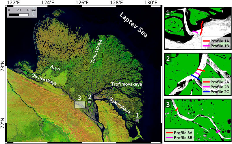
FIGURE 1. Mosaic of Landsat 8 OLI images (generated in Google Earth Engine) of the Lena River Delta with its numerous river channels. Three sites with in situ electrical resistivity tomography (ERT) profiles are shown in the inset maps with the synthetic aperture radar (SAR) winter backscatter image (median of several years) in the background and a land mask (green).

Methods

Remote Sensing

Two types of satellite remote sensing data were used in this study: 1) optical data from the Sentinel-2 Multispectral Instrument (MSI) and 2) SAR data from Sentinel-1 mission. Although we used both instruments to detect the same river ice features, the natural processes and remote sensing principles behind the two types of observations are different.

Optical Remote Sensing

Cloud-free optical satellite data (product type S2 MSI L1C) acquired by the Multispectral Instrument (MSI) on-board the Sentinel-2 satellite (S-2) were downloaded from the Copernicus Open Access Hub (https://scihub.copernicus.eu/dhus/). The reflectance for the selected profiles (along the GPS track of the ERT profiles) was extracted from two S-2 scenes (Table 1) using band 8 in the near infrared (∼833 nm), where the reflectance properties between ice and water differ most. For this study, we chose cloud-free S-2 scenes from late May/early June when the Lena River water level is highest and serpentine ice is present. Additionally, we used cloud-free S-2 imagery from the late summer (Sept. 1 to 2, 2016) during low water level to create a water mask for the low water in the Lena River.

TABLE 1

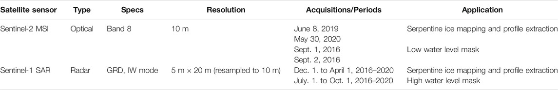
TABLE 1. List of remote sensing data used in the study.

Radar Remote Sensing

Radar data have the advantage of being independent of the cloud cover and polar night, and, therefore, one can explore the advantage of using multiple acquisitions over the focus area. Radar remote sensing has been employed since the 1970s to distinguish shallow and deep parts of Arctic lakes (e.g., Elachi et al., 1976), based on the distinctly different scattering properties from the bedfast ice and the ice resting on top of the unfrozen water mass. The method, however, has seldom been used for river ice.

The Sentinel-1 (S-1) mission began regular operation over the Lena Delta region in 2016, and since then, it has provided images from different overlapping orbits every 12 days. The large amount of S-1 data acquired so far allows for their temporal aggregation, which can substantially improve the visual quality and enhance the image features. We used Google Earth Engine (GEE) to process a large amount of S-1 data. For S-1, GEE provides the level-1 Ground Range Detected (GRD) product, which gives the calibrated, multilooked, and ortho-rectified backscattering coefficient. We used the Interferometric Wide (IW) Swath Mode, which originally featured 5 m × 20 m resolution, resampled in the GRD product to a pixel size of 10 by 10 m. We used three overlapping orbits, which, when combined, covered the entire Lena Delta and the adjacent coastal areas. Data in the IW mode is dual-polarized and consists of VV and VH polarization bands for the three orbits used here. We used the VH polarization band for the analysis as it showed a higher signal-to-noise ratio than VV band (Table 1). We used S-1 data for two purposes: 1) to produce a mask of river channels in summer, and 2) to delineate serpentine ice within the channels.

For producing the summer channel mask, we selected S-1 images only from the period when all river channels were free of ice. According to visual inspection, the period from July 1 to October 1 was a safe choice for all studied years, i.e. no ice was observed in the channels. We used the median backscatter of five summer seasons (2016–2020). Taking the median substantially decreased the noise and facilitated the subsequent classification into land and water classes. In general, the summer images featured distinctly lower backscatter over the water and over the sandbars as a result of specular signal reflection from smooth surfaces, compared to the higher backscatter over the vegetated upland. We used this observation to perform a simple unsupervised classification on the summer median backscatter to separate land from water and sandbars. Visual comparison with optical imagery confirmed the generally good performance of the classification. Because water and sandbars were practically indistinguishable in the SAR signal, the obtained S-1 summer channel mask can also represent the high water stand during the spring flood.

For the mapping of serpentine ice in the river channels, we selected the S-1 images from the winter period when all river channels were frozen. We defined the winter period as from December 1 to April 1. We confirmed visually that break-up did not happen before April 1 for all the studied years. Both serpentine ice and land appear bright on a winter S-1 backscatter image. To avoid confusion between those classes, we used the summer channel mask and excluded the land from the analysis. We classified the two types of ice (serpentine and bedfast) within the extent of the channels.

Geoelectrical Resistivity Surveys

The application of ERT can give us a representation of the geological structure and its state at different depths along the profile of measurements. The precondition for talik detection with direct current electrical resistivity is a substantial resistivity difference between thawed and frozen sediments (Kneisel et al., 2008; Hauck, 2013). Besides temperature, bulk sediment resistivity depends on sediment composition, unfrozen water content, ice content, and the presence of dissolved salts in the pore water. We applied continuous resistivity profiling (CRP), in which a floating electrode streamer was towed behind a small boat, making discrete vertical soundings at set spatial intervals. Positioning was via a global positioning system (GPS) at one end of the cable or streamer for each measurement (site 1: Garmin GPSMAP 64s; sites 2 and 3: Garmin GPSMAP 421, see Figure 1 for site locations). For CRP, an echo sounder measured water depth at each measurement. An IRIS Syscal Pro system was used to collect the data for all CRP measurements. The streamer was towed behind the boat and the cable floated on the water surface, with the help of regularly spaced buoys attached to the cable.

In CRP, current is injected into the water with two current electrodes and the voltage is measured with two potential electrodes. The calculated resistance is converted to an apparent resistivity using a geometric factor that depends on the configuration of the electrodes. The IRIS Syscal Pro has 10 channels to yield 10 apparent resistivities with different geometric factors at each sounding location almost simultaneously. The apparent resistivity is characteristic of a homogeneous subsurface and thus an inversion of the field data is needed to estimate the true distribution of the electrical resistivity in the ground.

The CRP at site 1 was measured on August 3, 2017 with a 120 m electrode streamer with electrodes arranged in a reciprocal Wenner-Schlumberger array. The electrodes, including the current electrodes, were spaced 10 m apart. Soundings were taken approximately every 20 m based on GPS position. A Sontek CastAway conductivity-temperature-depth (CTD) profiler was used to measure the water column electrical conductivity and temperature. CRP profiles were truncated to sections along which the cable was oriented in a straight line.

Measurements at site 2 were conducted from July 6 to July 14, 2017, at site 3 from July 6 to July 13, 2018. At sites 2 and 3, the towed streamer was 240 m long and a dipole-dipole electrode configuration was employed. The spacing of the current dipole was 20 m, the spacing of the potential dipoles varied from 10 to 40 m and the offsets varied from 25 to 200 m. At the beginning of cross-section profiles, the streamer was laid out on the beach. Despite the river current, the streamer was maintained in a roughly straight line. The CRP profiles 2A–2A’, 3A–3A’ and 3B–3B’ were complemented by stationary ERT soundings on the banks of the river, when the instrument was placed at the water edge. One cable with electrodes was submerged to the river bottom with the far end of the cable anchored by the boat and the other cable laid on the beach, both perpendicular to the shoreline. The results of CRP and stationary ERT measurements conducted along one survey line were then combined and inverted together.

The data from site 1 was processed using Aarhus Workbench software using a 1D laterally constrained inversion. Erroneous data points (outliers) for the outermost electrode pairs were removed from the dataset and no smoothing was applied. A standard deviation of 10% was set to the apparent resistivity data upon model import. The model consisted of 16 layers. The first layer thickness was set using the water depth and the first layer resistivity was set to 100 Ωm in accordance with the measured water electrical conductivity. For profile 1B–1B’, the water depths were taken from the echo-sounder. For profile 1A–1A’, the water depths were extracted from digitized nautical charts because the echo-sounder failed at many sounding locations. The CTD profile showed no stratification in the water column. We assigned a standard deviation of 10% to the water layer resistivity and left the remaining layer resistivities unconstrained in the inversion. Layer thicknesses were 1.1 m for the second layer and increased logarithmically with depth until 3.5 m at a depth of 30 m below the riverbed. Due to the wide spacing of soundings, the lateral constraint for resistivity was set to a standard deviation factor of 2.0. The vertical constraint on resistivity was set to a standard deviation factor of 4.0. The smooth inversion scheme was used to process the data, since we had no a priori information on the sediment properties for a few-layered inversion scheme. Default starting model resistivities were used and were the same everywhere in the model domain below the water layer. After the first inversion, modeled data points that fell outside the 10% error bar (forward modeled apparent resistivity outside apparent resistivity error range) were removed from the dataset if the data residual for a sounding was above 1.0. The inversion ran multiple times with reduced data points and the final result was such that each sounding had a data residual at or below 1.0 (i.e., the forward response fell within a 10% error bar on the observed data for each sounding).

Apparent resistivities at sites 2 and 3 were inverted with ZondRes2D software (http://zond-geo.com/english/zond-software/ert-and-ves/zondres2d/). A Smoothness constrained inversion with a Gauss-Newton algorithm was performed. Bathymetry data and water resistivity were included in the model as a priori information. A grid with 11 layers was used with layer thickness increasing logarithmically till a depth of about 70 m. Using a streamer twice as long as that used at site 1 increased the depth of investigation. The horizontal cell size was established in such a manner that the total number of cells was comparable to the total number of measurements to better stabilize the inversion. Joining of the cells in lower layers of the grid was also used, as the resolution of an electrical sounding decreases with depth. Then the same routine as for the data from site 1 was applied: two-stage inversion and exclusion of points for which the misfit exceeded 10% after the first run. The final root mean-squared error fell below three percent for all soundings from sites 2 and 3.

Numerical Modeling of Heat Flux

We use a 2D implementation of the permafrost model CryoGrid (Langer et al., 2016; Westermann et al., 2016) to simulate the temperature field below the Lena River. The model implementation used was defined at the upper boundary by a Dirichlet condition (surface temperature) while the lower boundary (∼600 m) was defined by a constant geothermal heat flux (Neumann condition). Turbulent heat transfer through the unfrozen water column was assumed, which was emulated by setting the water column to a uniform temperature equal to the surface temperature during the ice off period (Nitzbon et al., 2019) and 0°C during the ice on period. The model framework including lateral heat transfer has been shown to work well in differently sized lake settings (Langer et al., 2016). In contrast to lakes, a well-mixed water column beneath floating ice was assumed in the model setting. The model was forced with a combination of one-year of measured Lena River water temperatures (Juhls et al., 2020) for the flowing water and 20 years of Samoylov air temperatures (Boike et al., 2019) during periods of bedfast ice. Ice growth and therefore bedfast ice periods were simulated within the model. For both temperature records, we averaged the available data to generate a 1 year forcing with daily mean temperatures. The resulting annual forcing was repeated until the model reached a steady state after a model time of 2000 years. The equilibrium at this point was independent of the assumed temperature field at the beginning of the model period. The model made use of an implicit finite difference scheme to solve the heat equation with phase change, originally established by Swaminathan and Voller (1992). The model calculated the temperature field over a transect through the river channel using a lateral grid cell spacing of 5 m and a logarithmically increasing vertical grid cell spacing with depth. The sediment properties were assumed to be homogeneous over depth and lateral distance, with a sediment porosity of 40% and a mineral thermal conductivity of 3.8 W/(mK).

Results

Mapping Serpentine Ice Using Remote Sensing

Optical (spring) and radar (median winter) imagery showed very similar patterns in reflectance and SAR backscatter in the river channels (Figure 2). In the optical images, acquired in late May/early June, we observe high reflectance of light along serpentine ice surfaces, which is usually bordered on either side by low optical reflectance, corresponding to an ice-free water surface (Figure 2A). The SAR data (Figure 2B) features high backscatter in the deep central parts of the delta channels and low backscatter on either side where the ice is presumably frozen to the riverbed. Figure 2 also shows that serpentine ice is not limited to the inner part of the delta, but continues offshore around the delta where it becomes wider and finally dissipates. These offshore serpentine ice features can be several tens of kilometers long and describe the continuation of the river channels in the shallow near-shore waters surrounding the Lena River Delta. Additionally, the SAR data shows wide bedfast ice areas in these near-shore zones where water depths are below ∼2 m (maximum ice thickness in winter). Within the inner delta, serpentine ice covers most of the channel area. In contrast, toward the mouths of the channels, more relative bedfast ice area compared to floating ice (serpentine ice) is present where channels become wider.

FIGURE 2

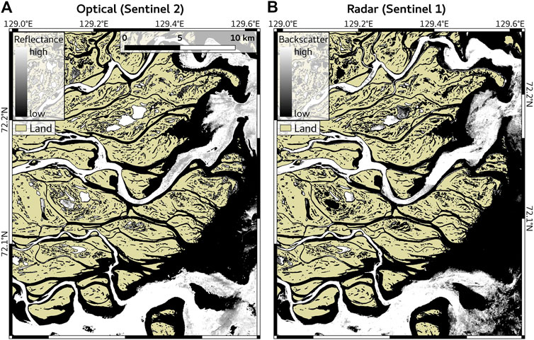
FIGURE 2. A) Optical Sentinel-2 satellite image (band 8) from June 8, 2019 and (B) SAR Sentinel-1 winter median image (2016–2020, December 1 to April 1) of an area at the mouth of the Bykovskaya and Trofimovskaya Channel in the eastern Lena River Delta. Serpentine ice over the deep parts of the channels is featured by high optical reflectance (A) and high SAR backscatter (B). Yellow filling shows the upland areas.

Here, we present the results of the mapping of three different areas within the river channels: channel area during the high water level, channel area during the low water stand, and the deep part of the channels where ice does not freeze to the bottom (i.e., serpentine ice) for the entire Lena River Delta. The map of channels during the high water level was created using summer SAR imagery, the map of channels during the low water level using summer optical imagery, and the map of serpentine ice, i.e., the deep part of channels, using winter SAR imagery (see Methods). The results show the minimum and maximum area of the Lena River Delta that is covered by channels. More importantly, the serpentine ice product shows parts of many channels that are frozen completely which results in an interruption of the channel connectivity to the sea (Figure 3). The importance of mapping channels that are characterized by bedfast ice for hydrological routing is further described and discussed in the section Connectivity of Lena River in Summer vs Winter. Furthermore, the mapping of deep channels along with water extents during different water levels can provide valuable information for navigation (discussed in the section Using Remote Sensing of the Serpentine Ice for Summer Navigation). A portion of the dataset is shown in Figure 3. Shapefiles of the presented products are available online (https://github.com/bjuhls/SerpChan).

FIGURE 3

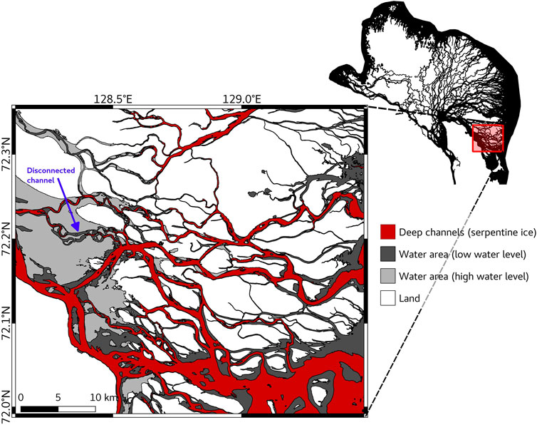
FIGURE 3. Selected region of the Lena River Delta showing the deep parts of the river channels (red; winter SAR imagery), channel area during low water period (dark gray; optical imagery), and channel area during high water level (light gray; summer SAR imagery).

Cross-Channel Profiles of Remote Sensing, Geoelectrical and Model Data

In order to investigate the relationship between the sub-river sediment conditions and the position of the serpentine ice in the river channels, we compare remote sensing observations (reflectance and backscatter), in situ ERT measurements, acquired during the field campaign in summers of 2017 and 2018, and a 2D thermal numerical model along the ERT profiles at three locations (Figures 4–6, Supplementary Figures S1–S4). While site 1 is located at the mouth of the Bykovskaya Channel, site 2 and site 3 are located in the central Lena River Delta (Figure 1).

FIGURE 4

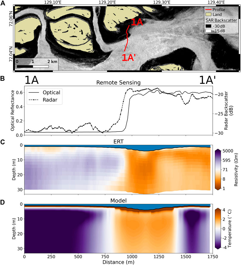
FIGURE 4. Profile (1A–1A’) (for the location see Figure 1). (A) GPS track of the ERT profile on top of the SAR Sentinel-1 median winter image showing the bedfast (dark) and serpentine (bright) ice. (B) Extracted optical reflectance and SAR backscatter along the profile. (C) Cross section of the inverted ERT resistivity along the profile. (D) Modeled sediment temperature along the profile.

Along the profile 1A–1A’ (Figure 4A), both optical reflectance and radar backscatter showed a pronounced increase at a distance of 900 m indicating a transition from bedfast ice to serpentine ice (Figure 4B). The ERT inversion results (Figure 4C) showed a lateral transition toward higher resistivity values also at a distance of 900 m. From 0 to 900 m, there was a high resistivity layer (100–1,000 Ωm) overlain by a thin mid-range resistivity layer (10–100 Ωm) below the water column. South of 900 m, the maximum resistivity in the sediment column was mostly below 10 Ωm until 1,200 m. Starting at 1,250 m, a low resistivity layer (<10 Ωm) was present from the riverbed until 10 m below water level (bwl) and gradually thickened from the riverbed to 20 m bwl at the end of the profile. The low resistivity layer was overlain by a thin mid-range resistivity layer (10–50 Ωm) <2 m thick just below the water layer in some areas. Furthermore, a mid-range resistivity layer (10–30 Ωm) was also observed below the low resistivity layer after 1,200 m. Despite shallow water depths indicative of highly probable bedfast ice conditions, no resistivities exceeded 100 Ωm, like those observed in the 0–900 m segment. The resistivities exceeding 100 Ωm could reveal the thermal impacts of bedfast ice in shallow areas with water depths between 1 and 2 m from 0 to 800 m and the presence of permafrost. In deeper water (e.g., at position 1,100 m), there is a substantially lower resistivity layer beneath the riverbed, suggesting the presence of unfrozen sediment.

The modeled sediment temperature (Figure 4D) showed cold temperatures (<−4°C) in the areas of shallow water (<800 m and >1,400 m) and a pronounced column of warm sediment temperatures (around 0°C) in the center of the profile, largely agreeing with the resistivity results. The low-resistivity and warm-sediment column is consistent with the position of the channels that is characterized by deeper water (≥2 m) compared to the surroundings (<2 m). The modeled sediment temperature after 1,400 m also reveals a frozen permafrost body beneath shallow waters (1.1 to 1.8 m deep), but the resistivity in the sediment column did not exceed 100 Ωm. Hence, the geophysical detection of permafrost along this segment is less certain and this anomaly is addressed in the discussion.

The model is sensitive to whether there is on-ice snow (and its thickness) and to the speed of ice removal during the spring flood. We ran different scenarios to quantify the impact of these two parameters on the temperature of the sediment beneath the riverbed and the position of the permafrost table beneath the talik. Allowing snow to accumulate on the river ice (from 0 m to 0.15 m) extended the talik size laterally (Supplementary Figure S5) and increased the talik temperature by up to 3°C.

The profile 2A–2A’, located in the central Lena Delta, crosses a channel of the Lena River almost completely (Figure 5). Both optical and SAR remote sensing data showed similar development along the profile, with high optical reflectance and high SAR backscatter over the serpentine ice (Figure 5B). Toward both ends of the profile, the optical reflectance and SAR backscatter dropped. In contrast to site 1 (Profile 1A–1A’ and 1B–1B’), this part of the channel does not have a distinctly visible area of bedfast ice but features a rather sharp transition between serpentine ice and land.

FIGURE 5

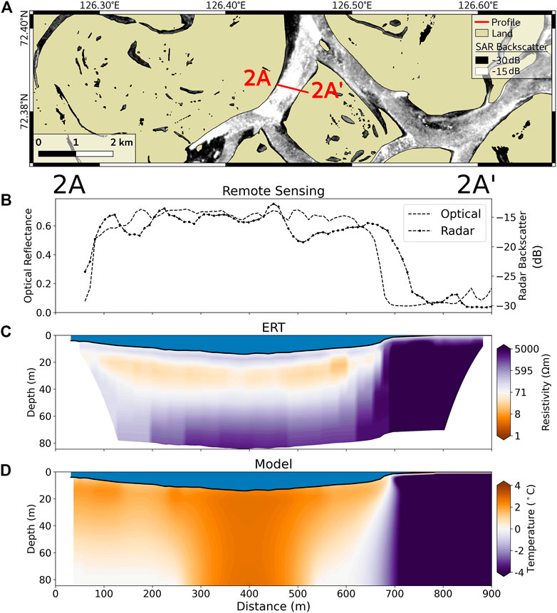
FIGURE 5. Profile (2A–2A’) (for the location see Figure 1). (A) GPS track of the ERT profile on top of the SAR Sentinel-1 median winter image showing the bedfast (dark) and serpentine (bright) ice. Note that bedfast ice is not present (or has minimal presence) on the profile (2A–2A’). (B) Extracted optical reflectance and SAR backscatter along the profile. (C) Cross section of the inverted ERT resistivity along the profile. (D) Modeled sediment temperature along the profile.

Similar to profile 1A–1A’, the ERT inversion results showed a closed low-resistivity zone in the sediment beneath the deep part of the river channels for the profile 2A–2A’. The low-resistivity zone (Figure 5C) generally showed slightly higher resistivities compared to profile 1A–1A’. Below the low-resistivity zone, resistivities >10 Ωm were observed. The eastern side of the profile (>700 m) showed higher resistivities (1,000–10,000 Ωm).

The modeled sediment temperature for profile 2A–2A’ (Figure 5D) showed low temperatures (<−4°C) beneath land on the eastern side. Across the whole river channel where water depth was >2 m, the sediment temperatures were positive with a zone of notably warmer sediment along the entire sediment column at the profile interval between 300 and 500 m. Toward the river shore, the lateral temperature gradient was more gradual as a function of depth. At a depth of 82 m, the sediment temperature decreased from >0°C at 500 m to −4°C at 700 m, whereas the same temperature differential spanned just several meters at the riverbed.

The profile 3B–3B’, which stretched across zones of bedfast ice, serpentine ice, and land (Figure 6A) generally affirmed the observations from the two other profiles. SAR backscatter (Figure 6B) showed generally lower backscatter (about 5 dB) over serpentine ice compared to the sites 1 and 2. Backscatter showed a gradual increase between 100 and 300 m of the profile, where presumably a transition between bedfast and serpentine ice occurs. The transition here is very smooth compared to the steep transitions from land or bedfast ice to serpentine ice in the profiles 1A–1A’ and 2A–2A’. This could be related to a lower slope in bathymetry and gradual bedfast freezing in winter, as well as to the interannual variability of the transition between bedfast and serpentine ice, as the median SAR backscatter from several winters is taken. Between 950 and 1,050 m of the profile, the water was shallow (about 0.6 m) whereas another deeper part (2.7 m) was present at 1,100 m before the profile entered land. The variations in the water depth (and as a result, in the ice thickness) are also reflected in the backscatter course over the interval between 950 and 1,100 m. We could not find a suitable optical image during the spring break up for this location.

FIGURE 6

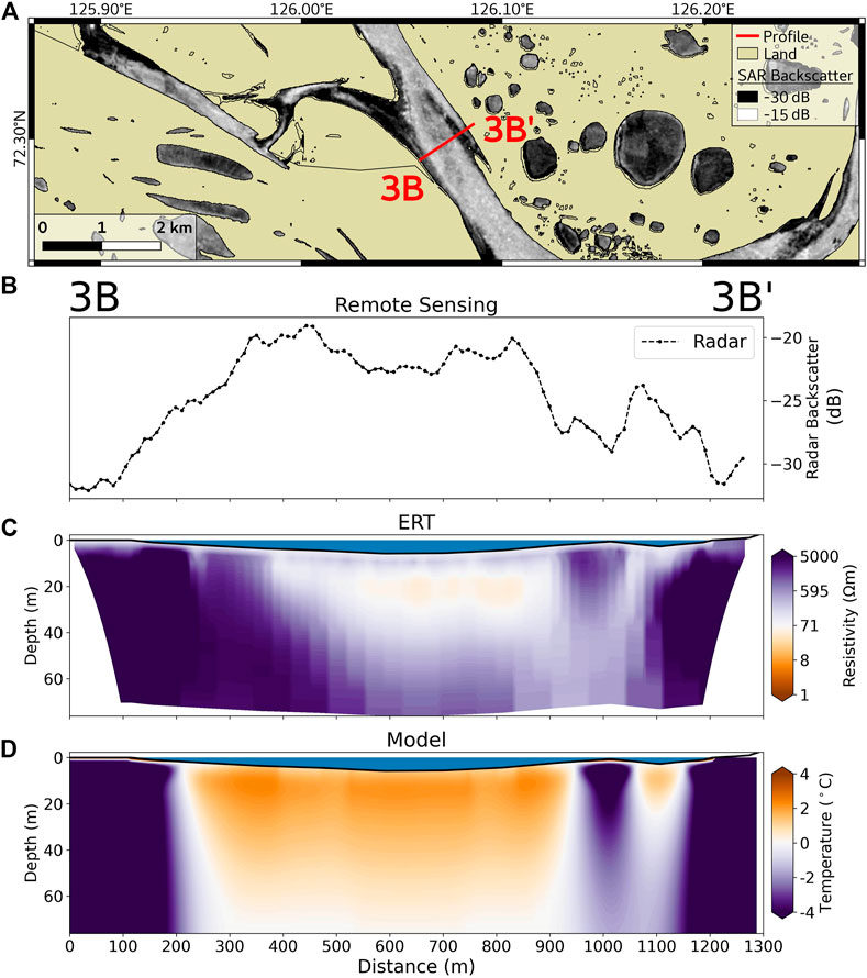
FIGURE 6. Profile (3B–3B’) (for the location see Figure 1). (A) GPS track of the ERT profile on top of the SAR Sentinel-1 median winter image showing the bedfast (dark) and serpentine (bright) ice. (B) Extracted SAR backscatter along the profile. (C) Cross section of the inverted ERT resistivity along the profile. (D) Modeled sediment temperature along the profile.

Profile 3B–3B’ was characterized by a more gradually decreasing water depth with respect to the shoreline compared to Profile 2A–A’. Correspondingly, the electrical resistivities of the sediment also decreased gradually from land to increasingly deep sub-aquatic conditions. On land, the resistivities exceeded 1,000 Ωm, and such conditions were sustained in shallow water areas within approximately 100 m of the riverbank. In addition, there was a localized region of high resistivity (>1,000 Ωm) beneath a sandbar at 1,100 m. There was a horizontally oriented oval-shaped low resistivity region (10–50 Ωm) from approximately 20–30 m bwl beneath the center of the channel. Outward of the perimeter of this minimum resistivity structure, the resistivities gradually increase in all directions away from it. Beneath the center of the channel, the resistivity started to exceed 100 Ωm at a depth of approximately 40 m.

The thermal modeling results corroborate the geophysical and remote sensing results for the terrestrial and shallow water areas. More specifically, the model showed cold permafrost temperatures (<−4°C) below land, bedfast ice areas within 100 m of the riverbank, as well as below the sandbar. However, the temperature field and permafrost distribution below the narrow sandbar were strongly affected by lateral heat fluxes. That is to say, the permafrost temperature beneath the sandbar started to increase above −4°C at a depth of 40 m, whereas the sub-aerial permafrost and sediment temperatures within 100 m of the southwestern riverbank were always below −4°C. Toward the northeast, the sediment temperatures were below −4°C within 50 m of the riverbank. Similar to profile 2A–2A’, the lateral temperature gradient was more gradual as a function of depth. Only between profile distances of 300–800 m was the entire sediment column just above 0°C and indicative of a talik.

Discussion

Serpentine Ice Formation and its Remote Sensing

We propose two possible explanations for the visibility of serpentine ice channels in spring with optical remote sensing (Figure 2A): 1) In winter, the ice growth in shallow waters is limited by the channel bottom. In deeper waters, the ice continues to grow and elastically bends upward, forced by the water beneath. During the spring flood, the elevated ice stays above water level, whereas the bedfast ice becomes submerged by the flood waters. 2) During the spring flood, the strong force of water flowing beneath the ice creates vertical cracks in the zone between bedfast ice and the ice in the deeper part of a channel. It is also possible that these cracks might be already formed by winter water level variations or by the tides in the coastal zones. The bedfast ice remains anchored while the flood waters penetrate through the cracks and submerge the bedfast ice. The ice over the deep part of the channel pops up along the cracks and floats, kept in place by the submerged bedfast ice from both sides.

In either case, the optical image shows low reflectance over flooded bedfast ice and high reflectance over the elevated surface of serpentine ice (Figure 7A). This situation can be observed during a relatively short time during spring flood, which typically lasts only a few days before all the ice is exported to the sea or melts.

FIGURE 7

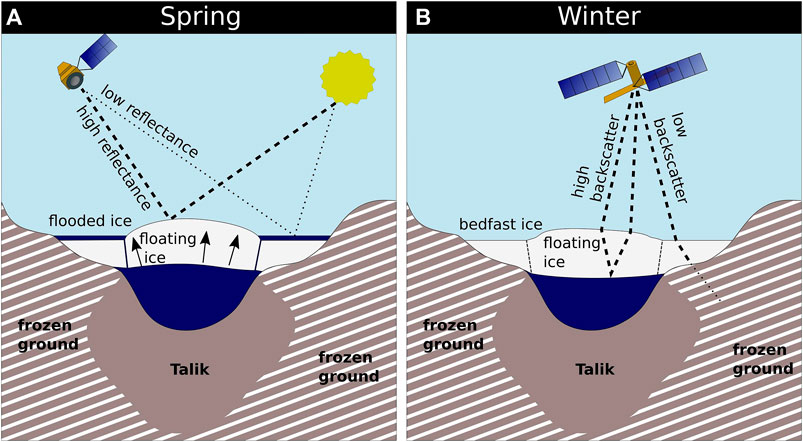
FIGURE 7. The sharp contrast in albedo between exposed serpentine ice and flooded bedfast ice is visible in optical imagery during the spring flood (A). In winter, the ice-water interface below serpentine ice is an effective reflector and produces a high radar backscatter signal (B).

The importance and timing of processes causing the serpentine ice to elevate above the flooded bedfast ice are not well studied or documented. In this study, we propose the two hypotheses, without providing observational proofs of the described processes (e.g., bending and cracking of ice). Previous studies however, suggested similar mechanisms for serpentine ice formation (Nalimov, 1995; Walker, 1998; Reimnitz, 2002).

The visibility of serpentine ice on winter SAR backscatter images (Figure 2A) can be explained by mechanisms which are studied and reported for many Arctic lakes (e.g., Elachi et al., 1976; Duguay et al., 2002; Atwood et al., 2015). Areas of low backscatter generally correspond to bedfast ice, and areas of high backscatter to floating, i.e., serpentine ice. Such distinct backscatter differences result from the interface that the SAR signal encounters after it has penetrated through the fresh ice. The SAR signal either dissipates into frozen bottom sediments under the bedfast ice, resulting in low backscatter, or scatters from the rough ice-water interface, resulting in high backscatter (Figure 7B). Based on reported ice thicknesses of the Lena River (Yang et al., 2002, 2021), zones of serpentine ice are restricted to regions with water depths greater than ∼1.5 m.

Generally, SAR remote sensing, which is independent of cloud coverage, seems to be a better tool to map serpentine ice/deep channels, compared to optical remote sensing. Considering the frequent cloud cover in the Arctic, it is well possible to miss the short-term event when relying only on optical remote sensing. Furthermore, the turbulent and chaotic processes during the river ice break-up can deform, dislocate or shatter the serpentine ice, making the use of optical imagery less reliable. An example of the disadvantage of optical reflectance compared to SAR backscatter is shown by the fact that we could not identify an optical S-2 image with a stable serpentine ice for profile 3B–3B’ (Figure 6). For this area, the serpentine ice on the optical image was already dislocated from its original position and did not correspond to the serpentine ice on the SAR image.

On the contrary, all available S-1 data from the whole winter period can be used for mapping exactly the same ice features. While temporal aggregation seems to be a good idea for smoothing and improving the contrast of the S-1 imagery, it is not strictly necessary, and even a single S-1 image can provide a sound distinction between bedfast and serpentine ice. A single S-1 image can provide a better snapshot of a situation in place and time and, therefore, can be used for the time series analysis, but suffers from noise and loses in quality to the temporal average.

Bartsch et al., 2017 show that the influence of incidence angle within the range of 29–46° (range of incidence angle for the S-1 IW mode used in this study) on the C-band backscatter is less than 2 dB. This is substantially lower than the backscatter difference between bedfast and floating ice (10–15 dB, Figures 4–6) shown in this study. Therefore, we did not apply an incidence angle normalization on the backscatter.

Implications of Changing Ice Thickness and Deep Channels for Permafrost Presence

In this study, we show that remote sensing can be used to map channels that are suitable for the formation of sub-river taliks in freshwater Arctic deltas and estuaries. Such taliks are interpreted to exist where serpentine ice persists for most of the winter. The sharp lateral transitions from low to high of both SAR backscatter and optical reflectance are in general well co-located with the sharp lateral transitions from high to low inverted bulk electrical resistivity in the sediment. The abrupt increase in resistivity is caused by a shift in the energy balance from the ice/riverbed to the water/riverbed interface. In regions of bedfast ice, heat flux is favored by the high thermal conductivity of the river ice coupling the riverbed to cold winter air temperatures. Beneath serpentine ice, two effects combine to prevent cooling of the riverbed: water provides an insulating layer between the river ice and the bed and heat is advected by water flow from lower latitudes (de Grandpré et al., 2012). In shallow areas where bedfast ice occurs, the sediment can cool rapidly due to atmosphere-riverbed coupling through the ice mass. This coupling can preserve permafrost if the ratio of freezing-degree-day to thawing-degree-day at the riverbed is sufficiently high, as demonstrated by Roy-Leveillee and Burn (2017) for thermokarst lakes. Atmosphere-riverbed coupling can also lead to permafrost aggradation in the case of substantial sediment deposition and consequent bedfasting of the ice in winter (Solomon et al., 2008). In the case of spits and sandbars near the river mouth, permafrost development would be even faster (Vasiliev et al., 2017). In any case, ground ice formation in the sediment results in an exponential increase in electrical resistivity for diverse sediment types (Overduin et al., 2012; Wu et al., 2017; Oldenborger, 2021). Although an electrical resistivity of 1,000 Ωm is commonly attributed to frozen sands with freshwater in the pore space (Fortier et al., 1994), values between 100–1,000 Ωm are reasonable for frozen silts (Holloway and Lewkowicz, 2019). The smooth minimum structure models we applied in the inversion mimic gradual geological transitions in the subsurface rather than sharply defined bodies (Auken and Christiansen, 2004). In the absence of salts, the low resistivity zones (900–1,200 m in profile 1A–1A’, Figure 4C, 100–700 m profile 2A–2A’, Figure 5C, and 250–900 m in profile 3B–3B’, Figure 6C) suggest a talik depth of at least 30 m bwl.

The formation of taliks at least 30 m bwl suggests that the location of the deep river channels in the Lena River Delta is stable. Based on visual inspection of optical remote sensing data with lower spatial resolution (MODIS) over 20 years (2000–2020, www.worldview.earthdata.nasa.gov), the serpentine ice channels occur at the same positions from year to year and vary only in their offshore extent, which can be explained by variability in the magnitude of coastal ice-flooding. While the delineation of floating and bedfast ice in thermokarst lakes using radar remote sensing (e.g., Antonova et al., 2016; Engram et al., 2018; Kohnert et al., 2018) and its potential for studying talik development (Arp et al., 2016) have been recognized, river channels and their ice regimes are largely overlooked. Long channels with reaches of tens to hundreds of kilometers with underlying taliks can form connections to deeper methane sources (Walter Anthony et al., 2012). Due to their spatial extent, the likelihood that river channel taliks cross geological pathways for gas migration such as the fault system along the southwestern edge of the Lena Delta is perhaps higher compared to lake taliks. Open taliks beneath paleo-river valleys have also been identified as possible pathways for methane release emanating from dissociating gas hydrates in subsea permafrost (e.g., Frederick and Buffett, 2014).

As ice thickness in the Arctic rivers tends to decrease with ongoing climate warming (Vuglinsky and Valatin, 2018) and projected increasing snowfall (e.g., Callaghan et al., 2011), the proportion of serpentine ice to bedfast ice area will likely increase, resulting in increased winter water flow beneath the ice (Gurevich, 2009; Tananaev et al., 2016), positive mean annual temperatures at a greater area of the riverbed and consequent talik growth. Sensitivity analysis of the model used in our study shows that even 5 cm of snow on the river ice can reduce the ice thickness at the end of the season by up to 30 cm, affect the thermal properties of the sub-river sediment, and cause talik growth (Supplementary Figure S5). Our results agree with a study on terrestrial permafrost from the Mackenzie Delta region of Canada, where ground surface temperature increased from approximately −24°C in wind-swept areas to −6°C in areas with 100 cm of snow (Smith, 1975).

While the inter-annual stability of channel position is partially due to permafrost formation beneath bedfast ice, atmospheric warming may also result in more dynamic bedload sediment transport and thus increased channel mobility (McNamara and Kane, 2009). We expect that the inter-annual variations in sediment load and ice thickness as well as the long-term trends for both variables can influence the bedfast/serpentine ice regimes and the thermal properties of the riverbed sediments only for the intermittently flooded sandbars and for shallow channels. In the deeper parts of channels, the water depth is in the order of tens of meters, which prevents such channels from migration and the sub-river talik from the influence of the ice thickness changes.

The gradual shift from a bedfast to serpentine ice regime may explain the mid-range electrical resistivity anomaly at distances greater than 1,200 m in profile 1A–1A’ (Figure 4). For this segment, the equilibrium thermal model state predicts permafrost temperatures as low as −4°C, despite the high optical reflectance and radar backscatter responses that are indicative of serpentine ice. The mid-range electrical resistivity zone (10–30 Ωm) is possibly a reflection of warming and degrading permafrost, compared to the high electrical resistivity zone (100–1,000 Ωm) north of 900 m. We interpret the latter to be colder permafrost sustained by a more stable perennially occurring bedfast ice regime. The profiles at site 1 have inverted resistivities near the riverbed of the central channel that are an order of magnitude lower (<10 Ωm) than those at sites 2 and 3 (<100 Ωm). Profile 1A–1A’ also showed lower resistivities in the talik (<10 Ωm) compared to profiles 2A–2A’ and 3A–3A’ (approximately 10–50 Ωm). We attribute the lower resistivities of the talik at the delta’s edge to possibly higher salt content in the sediment. We speculate that this is due to a number of processes including storm surges from Laptev Sea water, as well as groundwater flowing through taliks from upland areas to the nearshore zone. In fact, Fedorova et al. (2015) have suggested that infiltration of river water into taliks exerts a control on the delta’s discharge. Drawing on the research of Arctic perennial springs, flowing groundwater can mobilize salts and transport them to the outlet where they are deposited (Andersen, 2002).

Connectivity of Lena River in Summer vs Winter

The Lena River discharge in winter is substantially smaller (59 km³ for November–April) compared to summer (306 km³ for July–October) and spring (216 km³ for May–June) (Holmes et al., 2012). The map of serpentine ice for the whole delta (and, thus, the map of the deep channels) showed that the distribution of the water discharge through the channels also changes. Figure 8 shows that there are many channels that are disconnected in winter due to a complete freezing of the water column, at least as determined at the spatial resolution of the imagery used here. The total area of channels in the Lena River Delta (that have a connection to the sea) in winter (1,102 km²) is only 51% of what it is in summer (2,139 km²). Compared to the channel connectivity in summer, substantially fewer channels connected the main Lena River channel to the sea in winter (Figure 8). Only four large channels (Trofimofskaya, Bykovskaya, Olenekskaya and the Aryn Channel, Figure 1) stay active in winter, while most of the smaller channels, many of which connect the larger channels with each other, are disconnected due to freezing of the ice to the bed. Due to the limited spatial resolution of the remote sensing data (better than at least 20 m, Table 1), narrower channels may remain undetected by our method.

FIGURE 8

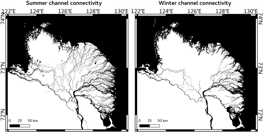
FIGURE 8. Sea-connected Lena River channels in summer during low water level (left) based on optical remote sensing data (Sentinel-2) and in winter (right) based on SAR remote sensing data (Sentinel-1).

The winter connectivity of channels and the under-ice water flow has an impact on the distribution and accumulation of the freshwater on the Laptev Sea during the ice-covered period. The interruption of flow through channels in the northern part of the Lena River Delta (Tumatskaya Channel) effectively turns off the winter under-ice freshwater supply to northern coastal waters. This may explain the observed high salinity (>20) and low turbidity of upper water beneath the landfast ice in winter compared to the outflow region east of the delta (Wegner et al., 2017; Hölemann et al., 2021). Furthermore, blocked channels probably play an important role for ice jams in the early stage of the freshet in spring (Beltaos et al., 2012; Kozlov and Kuleshov, 2019).

As climate warming drives permafrost thaw, groundwater will likely increase its contribution to the Lena River discharge (Frey and McClelland, 2009). Increasing active layer thickness and new groundwater flow pathways might be detectable by a long-term increase in winter base flow, which originates mostly from subsurface water (Juhls et al., 2020). Increasing winter discharge is observed for the Lena and other great Arctic Rivers (Yang et al., 2002; McClelland et al., 2006). The increased winter discharge is transported exclusively by the connected deep channels. Mapping active delta channels becomes, therefore, increasingly important, also as a baseline for future hydrological changes to Arctic river deltas and receiving coastal waters.

Using Remote Sensing of the Serpentine Ice for Summer Navigation

Through our own field experience in the Lena River Delta, it has not escaped our notice that the delineation of serpentine ice using remote sensing provides a means of mapping navigable channels. Shipping channels in coastal zones at the mouth of Arctic deltas are characterized by extremely shallow waters and river ice dynamics make nautical markings such as buoys impractical. We tested the Sentinel-1-based map of serpentine ice to navigate along the Olenekskaya Channel in the very western part of the Lena River Delta (see Figure 1 for the location) in summer 2016. The GPS track of the small ship (draft of 1.5 m) that was used for the travel to the western Laptev Sea followed exactly the serpentine ice course that was mapped with Sentinel-1 imagery (Figure 9). Whenever the ship deviated from the course defined by serpentine ice, it became grounded in the shoals. In particular, the serpentine ice map aided in navigation in the open coastal waters during the night.

FIGURE 9

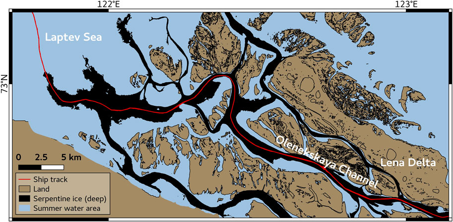
FIGURE 9. Track of a ship (red line) navigated in summer 2016 along the Olenekskaya Channel toward the western part of the Laptev Sea. A SAR-based map of serpentine ice was used for navigating along the deep parts of the channel, surrounded by extreme shallows (<1 m).

Currently, the Bykovskaya Channel (see Figure 1 for the location) is mostly used for regular shipping between the Laptev Sea and the upstream Lena River (www.marinetraffic.com). A direct routing from the western Laptev Sea to the main Lena River channel would save several hundreds of kilometers compared to the Bykovskaya Channel route. In consultation with local hydrographic services, the results of this study can, therefore, improve charts of traditional ship-based hydrographic surveys and ultimately the ship navigation in uncharted delta channels. Moreover, traditional hydrographic surveying techniques are costly and time consuming. In addition to mapping deeper parts of channels within the delta, we also map the prolongation of the deep channels offshore from the delta’s edge to the Laptev Sea. Our results demonstrate that annual-scale monitoring of the ice regime (bedfast vs serpentine) and the deep channels position is possible. These annual maps may be used as an aid for summer navigation for shallow-draught vessels, particularly in regions where navigational charts may not be regularly updated. The proposed mapping of deep river channels can be applied to other Arctic River deltas and estuaries, such as the Mackenzie Delta and the Kolyma estuary, that are characterized by shallow water depths at the river mouth and in the coastal zones. Current and future satellite missions will ensure regular updates of the maps to account for potential channel dynamics.

Conclusion

The bright elongated meandering river ice structures, detected on airborne photographs over several Arctic river deltas in the beginning of the spring break-up, were given the name of “serpentine ice” in the literature. In this study, we showed that SAR and optical remote sensing can be used to map the serpentine ice, which corresponds to the parts of the river channels that are deep enough not to freeze to the bottom throughout the winter. SAR backscatter from Sentinel-1 effectively distinguished serpentine ice from bedfast (frozen to the bottom) ice based on the different dielectric properties at the ice-water (in case of serpentine ice) and ice-frozen sediments (in case of bedfast ice) interfaces in winter. Optical reflectance from Sentinel-2 distinguished the highly reflective surfaces of elevated serpentine ice from strongly absorbing water on flooded bedfast ice in spring. By extending the remote sensing data with numerical thermal modeling and shallow geophysical data (ERT) acquired at several sites within the Lena River Delta, we showed that the distribution of bedfast and serpentine ice corresponds to the zones of frozen and thawed sediments beneath the riverbed. For river channels whose position remains stable over long periods of time, the presence of serpentine ice likely suggests the presence of a deep talik. The spatial correspondence between the river ice regime (bedfast or serpentine) and the thermal state of the sub-river sediments demonstrates the great potential of remote sensing to identify not only the long existing taliks beneath deep river channels but also areas, subject to potential change of the ice regime, which can, in turn, trigger either formation of new permafrost or thaw of existing permafrost beneath the riverbed.

Our map of serpentine ice provides new information about channels open to winter sub-ice flow and reveals how bedfast ice limits hydrological routing in winter compared to summer in the Lena River Delta. Our results can improve representation of river channel shape, sediment and matter dynamics, and ice-jamming in hydrological models. Moreover, our study shows how remote sensing can complement nautical charts to locate deep channels navigable for small ships.

Data Availability Statement

The original contributions presented in the study are included in the article/Supplementary Materials, further inquiries can be directed to the corresponding author. The data sets, codes and products of this study are available online (https://github.com/bjuhls/SerpChan).

Author Contributions

All authors contributed to the final design of the study. BJ and SA processed remote sensing data. PO, MA, NB, GM, and MG obtained and processed the geoelectrical data. FM and ML ran the model experiments. All authors contributed to the interpretation of data and writing of the manuscript.

Funding

This research was supported by the EU Horizon 2020 program (Nunataryuk, grant no. 773421). ERT data at the Olenekskaya Channel were obtained in the framework of the Russian Foundations for Basic Research project №18-05-60291. Projects from the BMBF-NERC’s Changing Arctic Ocean program (CACOON, NERC grant no. NE/R012806/1, BMBF grant no. 03F0806A) supported discussions within a larger group of experts.

Conflict of Interest

The author declares that the research was conducted in the absence of any commercial or financial relationships that could be construed as a potential conflict of interest.

The handling editor declared a shared research group (HORIZON2020 Nunataryuk) with one of the authors PPO at time of review.

Acknowledgments

Measurements at sites 2 and 3 were performed with the use of the equipment provided by the Research Park of St. Petersburg State University, Center for Geo-Environmental Research and Modeling (GEOMODEL). We are also grateful to the comments of two reviewers. I acknowledge support by the Open Access Publication Funds of Alfred-Wegener-Institut Helmholtz-Zentrum für Polar-und Meeresforschung.

Supplementary Material

The Supplementary Material for this article can be found online at: https://www.frontiersin.org/articles/10.3389/feart.2021.689941/full#supplementary-material

References

Ahmed, R., Prowse, T., Dibike, Y., Bonsal, B., and O’Neil, H. (2020). Recent Trends in Freshwater Influx to the Arctic Ocean from Four Major Arctic-Draining Rivers. Water 12, 1189. doi:10.3390/w12041189

CrossRef Full Text | Google Scholar

Alekseevskii, N. I., Aibulatov, D. N., Kuksina, L. V., and Chetverova, A. A. (2014). The Structure of Streams in the Lena delta and its Influence on Streamflow Transformation Processes. Geogr. Nat. Resour. 35, 63–70. doi:10.1134/S1875372814010090

CrossRef Full Text | Google Scholar

Andersen, D. T. (2002). Cold Springs in Permafrost on Earth and Mars. J. Geophys. Res. 107, 5015. doi:10.1029/2000JE001436

CrossRef Full Text | Google Scholar

Antonova, S., Duguay, C., Kääb, A., Heim, B., Langer, M., Westermann, S., et al. (2016). Monitoring Bedfast Ice and Ice Phenology in Lakes of the Lena River Delta Using TerraSAR-X Backscatter and Coherence Time Series. Remote Sensing 8, 903. doi:10.3390/rs8110903

CrossRef Full Text | Google Scholar

Arp, C. D., Cherry, J. E., Brown, D. R. N., Bondurant, A. C., and Endres, K. L. (2020). Observation-derived Ice Growth Curves Show Patterns and Trends in Maximum Ice Thickness and Safe Travel Duration of Alaskan Lakes and Rivers. Cryosphere 14, 3595–3609. doi:10.5194/tc-14-3595-2020

CrossRef Full Text | Google Scholar

Arp, C. D., Jones, B. M., Grosse, G., Bondurant, A. C., Romanovsky, V. E., Hinkel, K. M., et al. (2016). Threshold Sensitivity of Shallow Arctic Lakes and Sublake Permafrost to Changing winter Climate. Geophys. Res. Lett. 43, 6358–6365. doi:10.1002/2016GL068506

CrossRef Full Text | Google Scholar

Atwood, D. K., Gunn, G. E., Roussi, C., Wu, J., Duguay, C., and Sarabandi, K. (2015). Microwave Backscatter from Arctic Lake Ice and Polarimetric Implications. IEEE Trans. Geosci. Remote Sensing 53, 5972–5982. doi:10.1109/TGRS.2015.2429917

CrossRef Full Text | Google Scholar

Auken, E., and Christiansen, A. V. (2004). Layered and Laterally Constrained 2D Inversion of Resistivity Data. Geophysics 69, 752–761. doi:10.1190/1.1759461

CrossRef Full Text | Google Scholar

Bartsch, A., Pointner, G., Leibman, M. O., Dvornikov, Y. A., Khomutov, A. V., and Trofaier, A. M. (2017). Circumpolar Mapping of Ground-Fast Lake Ice. Front. Earth Sci. 5, 12. doi:10.3389/feart.2017.00012

CrossRef Full Text | Google Scholar

Beltaos, S., Carter, T., and Rowsell, R. (2012). Measurements and Analysis of Ice Breakup and Jamming Characteristics in the Mackenzie Delta, Canada. Cold Regions Sci. Techn. 82, 110–123. doi:10.1016/j.coldregions.2012.05.013

CrossRef Full Text | Google Scholar

Biskaborn, B. K., Smith, S. L., Noetzli, J., Matthes, H., Vieira, G., Streletskiy, D. A., et al. (2019). Permafrost Is Warming at a Global Scale. Nat. Commun. 10, 1–11. doi:10.1038/s41467-018-08240-4

PubMed Abstract | CrossRef Full Text | Google Scholar

Boike, J., Nitzbon, J., Anders, K., Grigoriev, M., Bolshiyanov, D., Langer, M., et al. (2019). A 16-year Record (2002-2017) of Permafrost, Active-Layer, and Meteorological Conditions at the Samoylov Island Arctic Permafrost Research Site, Lena River delta, Northern Siberia: An Opportunity to Validate Remote-Sensing Data and Land Surface, Snow, and Permafrost Models. Earth Syst. Sci. Data 11, 261–299. doi:10.5194/essd-11-261-2019

CrossRef Full Text | Google Scholar

Brown, D. R. N., Brinkman, T. J., Verbyla, D. L., Brown, C. L., Cold, H. S., and Hollingsworth, T. N. (2018). Changing River Ice Seasonality and Impacts on interior Alaskan Communities. Weather. Clim. Soc. 10, 625–640. doi:10.1175/WCAS-D-17-0101.1

CrossRef Full Text | Google Scholar

Callaghan, T. V., Johansson, M., Brown, R. D., Groisman, P. Y., Labba, N., Radionov, V., et al. (2011). The Changing Face of Arctic Snow Cover: A Synthesis of Observed and Projected Changes. Ambio 40, 17–31. doi:10.1007/s13280-011-0212-y

CrossRef Full Text | Google Scholar

Charkin, A. N., Pipko, I. I., Yu. Pavlova, G., Dudarev, O. V., Leusov, A. E., Barabanshchikov, Y. A., et al. (2020). Hydrochemistry and Isotopic Signatures of Subpermafrost Groundwater Discharge along the Eastern Slope of the Lena River Delta in the Laptev Sea. J. Hydrol. 590, 125515. doi:10.1016/j.jhydrol.2020.125515

CrossRef Full Text | Google Scholar

Charkin, A. N., Rutgers van der Loeff, M., Shakhova, N. E., Gustafsson, Ö., Dudarev, O. V., Cherepnev, M. S., et al. (2017). Discovery and Characterization of Submarine Groundwater Discharge in the Siberian Arctic Seas: a Case Study in the Buor-Khaya Gulf, Laptev Sea. Cryosphere 11, 2305–2327. doi:10.5194/tc-11-2305-2017

CrossRef Full Text | Google Scholar

Cooley, S. W., and Pavelsky, T. M. (2016). Spatial and Temporal Patterns in Arctic River Ice Breakup Revealed by Automated Ice Detection from MODIS Imagery. Remote Sensing Environ. 175, 310–322. doi:10.1016/j.rse.2016.01.004

CrossRef Full Text | Google Scholar

de Grandpré, I., Fortier, D., and Stephani, E. (2012). Degradation of Permafrost beneath a Road Embankment Enhanced by Heat Advected in groundwater 1. Can. J. Earth Sci. 49, 953–962. doi:10.1139/E2012-018

CrossRef Full Text | Google Scholar

Duguay, C. R., Pultz, T. J., Lafleur, P. M., and Drai, D. b. (2002). RADARSAT Backscatter Characteristics of Ice Growing on Shallow Sub-Arctic Lakes, Churchill, Manitoba, Canada. Hydrol. Process. 16, 1631–1644. doi:10.1002/hyp.1026

CrossRef Full Text | Google Scholar

Elachi, C., Bryan, M. L., and Weeks, W. F. (1976). Imaging Radar Observations of Frozen Arctic Lakes. Remote Sensing Environ. 5, 169–175. doi:10.1016/0034-4257(76)90047-X

CrossRef Full Text | Google Scholar

Engram, M., Arp, C. D., Jones, B. M., Ajadi, O. A., and Meyer, F. J. (2018). Analyzing Floating and Bedfast lake Ice Regimes across Arctic Alaska Using 25 years of Space-Borne SAR Imagery. Remote Sensing Environ. 209, 660–676. doi:10.1016/j.rse.2018.02.022

CrossRef Full Text | Google Scholar

Evans, S. G., and Ge, S. (2017). Contrasting Hydrogeologic Responses to Warming in Permafrost and Seasonally Frozen Ground Hillslopes. Geophys. Res. Lett. 44, 1803–1813. doi:10.1002/2016GL072009

CrossRef Full Text | Google Scholar

Fedorova, I., Chetverova, A., Bolshiyanov, D., Makarov, A., Boike, J., Heim, B., et al. (2015). Lena Delta Hydrology and Geochemistry: Long-Term Hydrological Data and Recent Field Observations. Biogeosciences 12, 345–363. doi:10.5194/bg-12-345-2015

CrossRef Full Text | Google Scholar

Fortier, R., Allard, M., and Seguin, M.-K. (1994). Effect of Physical Properties of Frozen Ground on Electrical Resistivity Logging. Cold Regions Sci. Techn. 22, 361–384. doi:10.1016/0165-232X(94)90021-3

CrossRef Full Text | Google Scholar

Frederick, J. M., and Buffett, B. A. (2014). Taliks in Relict Submarine Permafrost and Methane Hydrate Deposits: Pathways for Gas Escape under Present and Future Conditions. J. Geophys. Res. Earth Surf. 119, 106–122. doi:10.1002/2013JF002987

CrossRef Full Text | Google Scholar

Frey, K. E., and McClelland, J. W. (2009). Impacts of Permafrost Degradation on Arctic River Biogeochemistry. Hydrol. Process. 23, 169–182. doi:10.1002/hyp.7196

CrossRef Full Text | Google Scholar

Gurevich, E. V. (2009). Influence of Air Temperature on the River Runoff in winter (The Aldan River Catchment Case Study). Russ. Meteorol. Hydrol. 34, 628–633. doi:10.3103/S1068373909090088

CrossRef Full Text | Google Scholar

Hauck, C. (2013). New Concepts in Geophysical Surveying and Data Interpretation for Permafrost Terrain. Permafrost Periglac. Process. 24, 131–137. doi:10.1002/ppp.1774

CrossRef Full Text | Google Scholar

Hölemann, J. A., Juhls, B., Bauch, D., Janout, M., Koch, B. P., and Heim, B. (2021). The impact of the freeze–melt cycle of land-fast ice on the distribution of dissolved organic matter in the Laptev and East Siberian seas (Siberian Arctic). Biogeosciences 18 (12), 3637–3655. doi:10.5194/bg-18-3637-2021

CrossRef Full Text | Google Scholar

Holloway, J., and Lewkowicz, A. (2019). “Field and Laboratory Investigation of Electrical Resistivity-Temperature Relationships, Southern Northwest Territories,” in 18th International Conference on Cold Regions Engineering and 8th Canadian Permafrost Conference, Quebec City, QC, Canada (American Society of Civil Engineers (ASCE)), 64–72. doi:10.1061/9780784482599.008

CrossRef Full Text | Google Scholar

Holmes, R. M., McClelland, J. W., Peterson, B. J., Tank, S. E., Bulygina, E., Eglinton, T. I., et al. (2012). Seasonal and Annual Fluxes of Nutrients and Organic Matter from Large Rivers to the Arctic Ocean and Surrounding Seas. Estuaries and Coasts 35, 369–382. doi:10.1007/s12237-011-9386-6

CrossRef Full Text | Google Scholar

Ivanov, V. V., Piskun, A. A., and Korabel, R. A. (1983). Distribution of Runoff through the Main Channels of the Lena River Delta (In Russian). Tr. AANI (Proceedings AARI) 378, 59–71.

Google Scholar

Juhls, B., Stedmon, C. A., Morgenstern, A., Meyer, H., Hölemann, J., Heim, B., et al. (2020). Identifying Drivers of Seasonality in Lena River Biogeochemistry and Dissolved Organic Matter Fluxes. Front. Environ. Sci. 8, 53. doi:10.3389/fenvs.2020.00053

CrossRef Full Text | Google Scholar

Kneisel, C., Hauck, C., Fortier, R., and Moorman, B. (2008). Advances in Geophysical Methods for Permafrost Investigations. Permafrost Periglac. Process. 19, 157–178. doi:10.1002/ppp.616

CrossRef Full Text | Google Scholar

Kohnert, K., Juhls, B., Muster, S., Antonova, S., Serafimovich, A., Metzger, S., et al. (2018). Toward Understanding the Contribution of Waterbodies to the Methane Emissions of a Permafrost Landscape on a Regional Scale-A Case Study from the Mackenzie Delta, Canada. Glob. Change Biol. 24, 3976–3989. doi:10.1111/gcb.14289

PubMed Abstract | CrossRef Full Text | Google Scholar

Kohnert, K., Serafimovich, A., Metzger, S., Hartmann, J., and Sachs, T. (2017). Strong Geologic Methane Emissions from Discontinuous Terrestrial Permafrost in the Mackenzie Delta, Canada. Sci. Rep. 7, 1–6. doi:10.1038/s41598-017-05783-2

PubMed Abstract | CrossRef Full Text | Google Scholar

Kozlov, D. V., and Kuleshov, S. L. (2019). Multidimensional Data Analysis in the Assessment of Ice-Jam Formation in River Basins. Water Resour. 46, 152–159. doi:10.1134/S0097807819020088

CrossRef Full Text | Google Scholar

Langer, M., Westermann, S., Boike, J., Kirillin, G., Grosse, G., Peng, S., et al. (2016). Rapid Degradation of Permafrost underneath Waterbodies in Tundra Landscapes-Toward a Representation of Thermokarst in Land Surface Models. J. Geophys. Res. Earth Surf. 121, 2446–2470. doi:10.1002/2016JF003956

CrossRef Full Text | Google Scholar

Lauzon, R., Piliouras, A., and Rowland, J. C. (2019). Ice and Permafrost Effects on Delta Morphology and Channel Dynamics. Geophys. Res. Lett. 46, 6574–6582. doi:10.1029/2019GL082792

CrossRef Full Text | Google Scholar

McClelland, J. W., Déry, S. J., Peterson, B. J., Holmes, R. M., and Wood, E. F. (2006). A Pan-Arctic Evaluation of Changes in River Discharge during the Latter Half of the 20th century. Geophys. Res. Lett. 33, L06715. doi:10.1029/2006GL025753

CrossRef Full Text | Google Scholar

McNamara, J. P., and Kane, D. L. (2009). The Impact of a Shrinking Cryosphere on the Form of Arctic Alluvial Channels. Hydrol. Process. 23, 159–168. doi:10.1002/hyp.7199

CrossRef Full Text | Google Scholar

Nalimov, Y. V. (1995). “The Ice thermal Regime at Front Deltas of Rivers of the Laptev Sea,” in Rep Polar. Editors H. Kassens, D. Piepenburg, J. Thiede, L. Timokhov, H.-W. Hubberten, and S. M. Priamikov (Kiel, Germany: GEOMAR Forschungszentrum für marine Geowissenschaften).

Google Scholar

Nitzbon, J., Langer, M., Westermann, S., Martin, L., Aas, K. S., and Boike, J. (2019). Pathways of Ice-Wedge Degradation in Polygonal Tundra under Different Hydrological Conditions. The Cryosphere 13, 1089–1123. doi:10.5194/tc-13-1089-2019

CrossRef Full Text | Google Scholar

Oldenborger, G. A. (2021). Subzero Temperature Dependence of Electrical Conductivity for Permafrost Geophysics. Cold Regions Sci. Techn. 182, 103214. doi:10.1016/j.coldregions.2020.103214

CrossRef Full Text | Google Scholar

O’Neill, H. B., Roy‐Leveillee, P., Lebedeva, L., and Ling, F. (2020). Recent Advances (2010–2019) in the Study of Taliks. Permafr. Periglac. Process. 31, 346–357. doi:10.1002/ppp.2050

CrossRef Full Text | Google Scholar

Overduin, P. P., Westermann, S., Yoshikawa, K., Haberlau, T., Romanovsky, V., and Wetterich, S. (2012). Geoelectric Observations of the Degradation of Nearshore Submarine Permafrost at Barrow (Alaskan Beaufort Sea). J. Geophys. Res. 117. doi:10.1029/2011JF002088

CrossRef Full Text | Google Scholar

Park, H., Watanabe, E., Kim, Y., Polyakov, I., Oshima, K., Zhang, X., et al. (2020). Increasing Riverine Heat Influx Triggers Arctic Sea Ice Decline and Oceanic and Atmospheric Warming. Sci. Adv. 6, eabc4699. doi:10.1126/SCIADV.ABC4699

PubMed Abstract | CrossRef Full Text | Google Scholar

Park, H., Yoshikawa, Y., Oshima, K., Kim, Y., Ngo-Duc, T., Kimball, J. S., et al. (2016). Quantification of Warming Climate-Induced Changes in Terrestrial Arctic River Ice Thickness and Phenology. J. Clim. 29, 1733–1754. doi:10.1175/JCLI-D-15-0569.1

CrossRef Full Text | Google Scholar

Piliouras, A., and Rowland, J. C. (2020). Arctic River Delta Morphologic Variability and Implications for Riverine Fluxes to the Coast. J. Geophys. Res. Earth Surf. 125. doi:10.1029/2019JF005250

CrossRef Full Text | Google Scholar

Prowse, T., Alfredsen, K., Beltaos, S., Bonsal, B., Duguay, C., Korhola, A., et al. (2011). Past and Future Changes in Arctic Lake and River Ice. Ambio 40, 53–62. doi:10.1007/s13280-011-0216-7

CrossRef Full Text | Google Scholar

Reimnitz, E. (2002). lnteractions of River Discharge with Sea lce in Proximity of Arctic Deltas: A Review, Polarforschung 70, 123–134.

Google Scholar

Rokaya, P., Budhathoki, S., and Lindenschmidt, K.-E. (2018a). Ice-jam Flood Research: a Scoping Review. Nat. Hazards 94, 1439–1457. doi:10.1007/s11069-018-3455-0

CrossRef Full Text | Google Scholar

Rokaya, P., Budhathoki, S., and Lindenschmidt, K.-E. (2018b). Trends in the Timing and Magnitude of Ice-Jam Floods in Canada. Sci. Rep. 8, 5834. doi:10.1038/s41598-018-24057-z

CrossRef Full Text | Google Scholar

Roy-Leveillee, P., and Burn, C. R. (2017). Near-shore Talik Development beneath Shallow Water in Expanding Thermokarst Lakes, Old Crow Flats, Yukon. J. Geophys. Res. Earth Surf. 122, 1070–1089. doi:10.1002/2016JF004022

CrossRef Full Text | Google Scholar

Schneider, J., Grosse, G., and Wagner, D. (2009). Land Cover Classification of Tundra Environments in the Arctic Lena Delta Based on Landsat 7 ETM+ Data and its Application for Upscaling of Methane Emissions. Remote Sensing Environ. 113, 380–391. doi:10.1016/j.rse.2008.10.013

CrossRef Full Text | Google Scholar

Shiklomanov, A. I., and Lammers, R. B. (2014). River Ice Responses to a Warming Arctic-Recent Evidence from Russian Rivers. Environ. Res. Lett. 9, 035008. doi:10.1088/1748-9326/9/3/035008

CrossRef Full Text | Google Scholar

Smith, M. W. (1975). Microclimatic Influences on Ground Temperatures and Permafrost Distribution, Mackenzie Delta, Northwest Territories. Can. J. Earth Sci. 12, 1421–1438. doi:10.1139/e75-129

CrossRef Full Text | Google Scholar

Solomon, S. M., Taylor, A. E., and Stevens, C. W. (2008). Nearshore Ground Temperatures, Seasonal Ice Bonding, and Permafrost Formation Within the Bottom-Fast Ice Zone, Mackenzie Delta, NWT. Proceedings of the Ninth International Conference on Permafrost, Fairbanks, AK, United States Fairbanks, Alaska

Google Scholar

Stephani, E., Drage, J., Miller, D., Jones, B. M., and Kanevskiy, M. (2020). Taliks, Cryopegs, and Permafrost Dynamics Related to Channel Migration, Colville River Delta, Alaska. Permafrost and Periglac Process 31, 239–254. doi:10.1002/ppp.2046

CrossRef Full Text | Google Scholar

Swaminathan, C. R., and Voller, V. R. (1992). A General Enthalpy Method for Modeling Solidification Processes. Mtb 23, 651–664. doi:10.1007/BF02649725

CrossRef Full Text | Google Scholar

Tananaev, N. I., Makarieva, O. M., and Lebedeva, L. S. (2016). Trends in Annual and Extreme Flows in the Lena River basin, Northern Eurasia. Geophys. Res. Lett. 43 (10), 764–772. doi:10.1002/2016GL070796

CrossRef Full Text | Google Scholar

Vasiliev, A. A., Melnikov, V. P., Streletskaya, I. D., and Oblogov, G. E. (2017). Permafrost Aggradation and Methane Production in Low Accumulative Laidas (Tidal Flats) of the Kara Sea. Dokl. Earth Sc. 476, 1069–1072. doi:10.1134/S1028334X17090203

CrossRef Full Text | Google Scholar

Vuglinsky, V., and Valatin, D. (2018). Changes in Ice Cover Duration and Maximum Ice Thickness for Rivers and Lakes in the Asian Part of Russia. Nr 09, 73–87. doi:10.4236/nr.2018.93006

CrossRef Full Text | Google Scholar

Walker, H. J., and Hudson, P. F. (2003). Hydrologic and Geomorphic Processes in the Colville River delta, Alaska. Geomorphology 56, 291–303. doi:10.1016/S0169-555X(03)00157-0

CrossRef Full Text | Google Scholar

Walker, H. J. (1973). Spring Discharge of an Arctic River Determined from Salinity Measurements beneath Sea Ice. Water Resour. Res. 9, 474–480. doi:10.1029/WR009i002p00474

CrossRef Full Text | Google Scholar

Walker, H. J. (1998). Arctic Deltas. J. Coast. Res. 14, 718–738.

Google Scholar

Walter Anthony, K. M., Anthony, P., Grosse, G., and Chanton, J. (2012). Geologic Methane Seeps along Boundaries of Arctic Permafrost Thaw and Melting Glaciers. Nat. Geosci 5, 419–426. doi:10.1038/ngeo1480

CrossRef Full Text | Google Scholar

Wegner, C., Wittbrodt, K., Hölemann, J. A., Janout, M. A., Krumpen, T., Selyuzhenok, V., et al. (2017). Sediment Entrainment into Sea Ice and Transport in the Transpolar Drift: A Case Study from the Laptev Sea in winter 2011/2012. Continental Shelf Res. 141, 1–10. doi:10.1016/j.csr.2017.04.010

CrossRef Full Text | Google Scholar

Westermann, S., Langer, M., Boike, J., Heikenfeld, M., Peter, M., Etzelmüller, B., et al. (2016). Simulating the thermal Regime and Thaw Processes of Ice-Rich Permafrost Ground with the Land-Surface Model CryoGrid 3. Geosci. Model. Dev. 9, 523–546. doi:10.5194/gmd-9-523-2016

CrossRef Full Text | Google Scholar

Woo, M. k. (1986). Permafrost Hydrology in North America1. Atmosphere-Ocean 24 (3), 201–234. doi:10.1080/07055900.1986.9649248

CrossRef Full Text | Google Scholar

Wu, Y., Nakagawa, S., Kneafsey, T. J., Dafflon, B., and Hubbard, S. (2017). Electrical and Seismic Response of saline Permafrost Soil during Freeze - Thaw Transition. J. Appl. Geophys. 146, 16–26. doi:10.1016/j.jappgeo.2017.08.008

CrossRef Full Text | Google Scholar

Yang, D., Kane, D. L., Hinzman, L. D., Zhang, X., Zhang, T., and Ye, H. (2002). Siberian Lena River Hydrologic Regime and Recent Change. J.-Geophys.-Res. 107, 14. ACL 14-1-ACL 14-1. doi:10.1029/2002JD002542

CrossRef Full Text | Google Scholar

Yang, D., Park, H., Prowse, T., Shiklomanov, A., and McLeod, E. (2021). “River Ice Processes and Changes Across the Northern Regions,” in Arctic Hydrology, Permafrost and EcosystemsEditors D. L. Kane, and K. M. Hinkel (Springer International Publishing), 379–406. doi:10.1007/978-3-030-50930-9_13

CrossRef Full Text | Google Scholar

Zheng, L., Overeem, I., Wang, K., and Clow, G. D. (2019). Changing Arctic River Dynamics Cause Localized Permafrost Thaw. J. Geophys. Res. Earth Surf. 124, 2324–2344. doi:10.1029/2019JF005060

CrossRef Full Text | Google Scholar