The New Swiss Glacier Inventory SGI2016: From a Topographical to a Glaciological Dataset

Introduction

Grosser Aletschgletscher is known to be the largest glacier in the Alps (Jouvet and Huss, 2019; GLAMOS, 1881-2020). Glacier length or ice volume are data to support this claim, but intuitively the easiest and most accessible measure is surface area – which amounts to 78.49 km² for Grosser Aletschgletscher. However, where does this number come from? How has this value been derived, and to which point in time does this glacier size correspond to? Such questions may be answered with a glacier inventory that provides “a detailed record of attributes of the glaciers in a region” (Cogley et al., 2011).

Repeated inventories are a key task to monitor the totality of glacier changes for an extent beyond a single glacier (Haeberli, 2004; Zemp et al., 2014) and provide detailed information on the glacier extent and additional important parameters such as area, elevation range, slope, aspect etc. for a given point or period in time (Paul et al., 2009). With increasing anthropogenic greenhouse gas emissions and corresponding global warming, glaciers in Switzerland are shrinking rapidly as in many mountain ranges on Earth (Zemp et al., 2015, 2019; Haeberli et al., 2019; Wouters et al., 2019; Hugonnet et al., 2021). Detailed information on glacier coverage is not only needed to quantify glacier area, but is also required for a wide range of glaciological and hydrological applications ranging e.g. from glacier-change assessments, mass balance and ice volume estimates, past, present and future runoff as well as projections of glacier mass loss to sea-level rise (Jacob et al., 2012; Bliss et al., 2014; Eis et al., 2019; Hock et al., 2019; McNabb et al., 2019; Grab et al., 2021). A frequent update of glacier inventories is required to respond to these fast changes in order to track rapid current and future glacier changes (Haeberli and Barry, 2006; Zemp et al., 2014).

Satellite images with sufficient spatial resolution (e.g. 30 m Landsat Thematic Mapper (TM)) have been widely used to map glacier extents in various parts of the world, partly using automated mapping of bare ice from multispectral image band ratios (Raup et al., 2007). The so derived glacier outlines were collected in the Global Land Ice Measurements from Space (GLIMS) database (Kargel et al., 2005) and often constituted a first initial representation of the glacier extent. The free availability of orthorectified Landsat images in 2008 (Wulder et al., 2012) enhanced mapping of glacier extents over increasingly large regions, often also including change assessment (e.g. Andreassen et al., 2008; Bolch et al., 2010; Paul et al., 2011; Rastner et al., 2012). These studies were accompanied by tutorials (Raup and Khalsa, 2010) and guidelines (Paul et al., 2009; Racoviteanu et al., 2009) to have some consistency in the generated data sets and the estimate of uncertainties (Paul et al., 2013). A first complete vector data set of glacier outlines worldwide was achieved with the Randolph Glacier Inventory (RGI) (Pfeffer et al., 2014) as a baseline for climate change impact assessments in IPCC AR5 (Vaughan et al., 2013). Since then, the RGI was repeatedly updated and improved in quality (RGI Consortium, 2017). Automated mapping of bare ice with multispectral classification methods is reliable, but outlines for debris-covered parts of glaciers still are mostly delineated manually (Paul, 2017). Despite the high workload, new data sets are constantly produced (mostly based on Landsat TM data and more recently with Sentinel-2 images) and made available via GLIMS (e.g. Nuth et al., 2013; Kienholz et al., 2015; Nuimura et al., 2015; Earl and Gardner, 2016; Barcaza et al., 2017; Meier et al., 2018; Mölg et al., 2018; Carrivick et al., 2020). Correct delineation of debris-covered glaciers is decisive for detecting glacier changes (Scherler et al., 2011) and information on debris extent should thus be included in large-scale glacier inventories, also providing a key to enhanced process understanding (Kraaijenbrink et al., 2017; Scherler et al., 2018; Herreid and Pellicciotti, 2020; Rounce et al., 2021).

In Switzerland, topographical mapping has a long-standing tradition (Rickenbacher and Just, 2012). The Swiss national topographic maps in different scales produced by the Federal Office of Topography (swisstopo) are famous for their precision, level of detail and temporal consistency. Starting from the Dufour Map (1844–1864) to the Siegfried Map (1870–1926) and all the following releases of national topographic maps (swisstopo, 2020d), swisstopo always sought to generate high precision topographical and geospatial information covering entire Switzerland, based on the latest technologies. Of course, also the glaciers have been mapped by swisstopo (Rastner et al., 2016; Freudiger et al., 2018), since the 1940s based on aerial images which can easily be examined online (swisstopo, 2020b).

Glacier monitoring in Switzerland goes back to the time of the earliest topographic maps (Siegfried map). Thereafter, topographic map sheets have been used for various glaciological studies and fieldwork. The need of glacier area data and the availability of the first complete detailed map series resulted in two early planimetric assessments of glacier coverage in the Swiss Alps (Jegerlehner, 1902; EAW, 1954). Based on the topographical maps and aerial images acquired by swisstopo, the Swiss Glacier Inventories (SGIs) SGI1850 (Maisch et al., 2000), SGI1973 (Müller et al., 1976) and SGI2010 (Fischer et al., 2014) were produced. Even though these past inventories are derivatives from swisstopo data, they have so far not been co-produced by topographers and glaciologists. The compilation of Swiss Glacier Inventories was not an institutionalized task, rather was based on research projects and individual initiatives (Müller et al., 1976; Maisch et al., 2000; Paul, 2004; Fischer et al., 2014; Freudiger et al., 2018).

Since 2016, the task to regularly produce updated glacier inventories was assigned to Glacier Monitoring in Switzerland (GLAMOS www.glamos.ch). Within defined time intervals (3–6 yr), swisstopo acquires high-quality aerial images, digital elevation models (DEMs) and topographical maps. These products include mapping of all ground surface types, including “glaciers” and “debris” (also on glacier ice), are available to GLAMOS, and serve as a basis to compile repeated and high-resolution glacier inventories for Switzerland.

Paul et al. (2011) presented a glacier inventory for the entire Alps compiled from Landsat satellite images acquired within a period of 6 wk in summer 2003. This data set is methodologically and temporarily consistent and represents the glacier outlines of the Alps in the latest version of the RGI (RGI Consortium, 2017). On a national level, detailed glacier inventories were compiled from high-resolution data sets (aerial photographs, airborne laser scanning). These national inventories refer to the periods 2008–2011 for Switzerland (SGI2010, Fischer et al., 2014), 2004–2011 for Austria (Fischer et al., 2015a), 2006–2009 for France (Gardent et al., 2014) and 2005–2011 for Italy (Smiraglia et al., 2015). Based on satellite imagery from Sentinel-2 and the national inventories as a guideline for interpretation, Paul et al. (2020) compiled a new inventory for the Alps referring to the year 2015 based on semi-automated mapping. The alpine-wide glacier inventories of 2003 and 2015 are methodologically consistent, and an overall change assessment reveals an area loss of 300 km² or 15%, but a glacier-by-glacier comparison was not possible (Paul et al., 2020). Half of the alpine-wide area change (–151 km²) during this 12-yr period can be assigned to Swiss glaciers. For the time of the end of the Little Ice Age, the SGI1850 reports a total glacier surface area of 1,788 km² (Maisch et al., 2000) that decreased to 1,311 km² as mapped within the SGI1973 (Müller et al., 1976). Fischer et al. (2014) reported a glacier area of 944 km² for the SGI2010, leading to an area change of –367 km² for the time period 1973–2010. All these inventories for the Swiss Alps (SGI1850, SGI1973 & SGI2010; Alps-2003 & Alps-2015) are accessible via the GLIMS glacier database.

The extent of debris-covered glacier surfaces is difficult to be detected with automated procedures and was not specifically mapped in any of the previous Swiss Glacier Inventories. Whether using satellite images or aerial photographs, compiling glacier inventories is a challenging task with a high workload (e.g., Barcaza et al., 2017; Mölg et al., 2018). Even if there is additional information (e.g., coherence images, Frey et al., 2012) or elevation differences (e.g., Abermann et al., 2010; Thompson et al., 2016; Mölg et al., 2019, 2020) that help delineating parts of glaciers that are covered by supraglacial debris, manual interaction is indispensable, requires expert knowledge and is still challenging, above all when only mapping in 2D-views (Herreid and Pellicciotti, 2020). Therefore, the accuracy of resulting glacier inventories is highly dependent on the quality and spatial resolution of data sources used, mapping tools applied, and finally based on subjective decisions taken by the operator (Fischer et al., 2014). In addition, “the on-going glacier decline also results in increasingly difficult glacier identification (under debris cover) and topologic challenges for a database (when glaciers split)” (Paul et al., 2020).

Hence, trying to assess individual and region-wide glacier changes asks for repeated, highly accurate and consistent glacier inventories that are based on defined methodologies and guidelines. A digitization with professional tools (3D-mapping) and trained topographers assures a high reproducibility. Storing a glacier inventory in a topological database with systematic, defined unique identifiers (IDs) allows tracing the evolution of parent glaciers after splitting into individuals and enables the derivation of glacier-specific area changes. Moreover, when mapping glaciers and supraglacial debris in different topological classes, the information on debris coverage can be added to the glacier inventory as additional spatial information. Swisstopo has the capacities, resources, methodologies, knowledge, tools and the official task to create layers of various geographical, topographical and topological information from high-resolution aerial photographs and DEMs, which are subsequently combined for the creation of topographic maps, where glacierized surfaces are represented too. However, a further control by glaciologists is required to derive a glacier inventory that fits glaciological criteria (e.g. glacier definition) according to Cogley et al. (2011).

In this study we present the new Swiss Glacier Inventory SGI2016, created based on high-resolution aerial imagery and digital elevation models. Glacier outlines of the SGI2016 were derived in close cooperation with swisstopo and GLAMOS, bringing together topographical and glaciological knowhow. The new and highly detailed data set is based on swisstopo’s object class “glacier” and additionally provides spatial information about debris cover by the intersection with the object class “debris” from the digital Swiss Topographic Landscape Model (swissTLM^3D). This allows analyzing, for example, the dependencies between topographic parameters and debris-cover fraction for individual glaciers. Furthermore, adoption of the same unambiguous coding scheme as applied in earlier Swiss Glacier Inventories allows detailed change assessments and, hence, insights into the processes driving changes of individual glaciers. The workflow developed for the creation of the SGI2016 is reproducible and will be applied again for the creation of future Swiss Glacier Inventories. The SGI2016 is the first step towards a consistent and accurate data product of repeated Swiss Glacier Inventories in 6-yr time intervals, which allows a high comparability of individual glaciers and glacier samples and will be available via the GLIMS database after publication.

Study Region and Data Sets

Study Region

In Switzerland, the Alps cover about two thirds of the country’s total area. They are thus a defining element of the landscape and an important factor for the identity of the people. The majority of the Swiss glaciers is located in the Valais, Bernese and Central Swiss Alps. The Eastern Swiss Alps harbor fewer glaciers, with exception of the southern Grisons Alps (Maisch et al., 2000). The SGI2010 reports a total of 1,420 glacier entities resulting in a total glacierized area of 944 ± 24 km² (Fischer et al., 2014).

Runoff from the Swiss Alps (and glaciers) feeds into five major European river catchments (Figure 1): Rhine, Rhone, Po, Adige and Danube, draining into the North Sea, the Mediterranean Sea, the Adriatic Sea and the Black Sea (Viviroli and Weingartner, 2004). The Swiss hydrological catchments with the highest glacierization contribute to an important extent to runoff to the two rivers Rhone and Rhine (Huss, 2011). Most of the glaciers in number are located in the Rhine catchment (including the tributary catchments of Aare, Reuss and Linth/Limmat), whereas in the Rhone catchment the glacierization is highest in absolute and relative terms. The very small part of the Adige catchment in Switzerland has no more any glacierization.

FIGURE 1

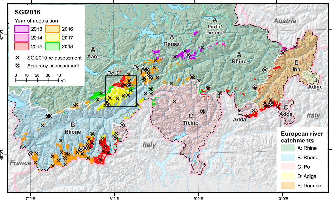
FIGURE 1. Overview of glacierization and main hydrological catchments in Switzerland. The Swiss contribution to the five major European streams Rhine (A, green), Rhone (B, blue), Po (C, red), Adige (D, yellow) and Danube (E, orange) is illustrated. The catchment borders are marked with a white line. The glacierization is illustrated by the new SGI2016 (this study), and colors refer to the year of acquisition of the aerial image used for glacier mapping. The sample of 100 glaciers used for a re-assessment of the SGI2010 (crosses) and the 15 glaciers used for the accuracy assessment (circled crosses) are indicated. The small rectangles show the extents enlarged in Figures 2, 5.

The size class distribution of Swiss glaciers is spatially variable and inhomogeneous. The number of glaciers is dominated by small and very small glaciers. In terms of total glacierization, these glaciers are of minor importance compared to the much less frequent, but larger mountain and valley glaciers (cf. Fischer et al., 2014).

Previous Inventories of Swiss Glaciers

Several inventories have been created for Swiss glaciers based on different methodologies and data sources. All of these data sets are as accurate as possible, reflecting the possibilities and technologies available at the time of their establishment. In principle, the data sets can be divided into two classes: inventories based on 1) maps, aerial images and manual digitization of glacier outlines, and 2) satellite images and semiautomatic mapping (Figure 2). The two classes also differ in their spatial resolution, which is generally coarser for 2).

FIGURE 2

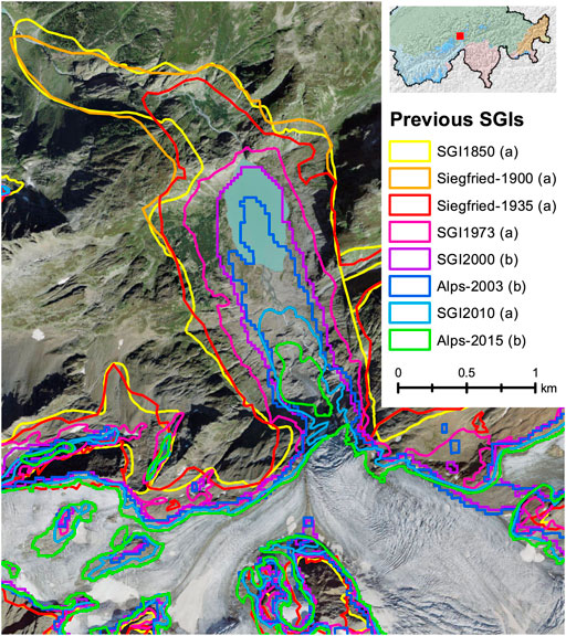
FIGURE 2. Compilation of glacier outlines from previous inventories available in digital format of Swiss glaciers for the example of Triftgletscher, Central Switzerland. Glacier outlines are in general either based on (a) maps, aerial images and manual digitizing, or (b) satellite images and semi-automated mapping. In the background, a SWISSIMAGE orthophoto acquired in 2018 is shown. The location within Switzerland is indicated in the inset (red rectangle).

SGI1973 and SGI1850

The first Swiss Glacier Inventory was derived from aerial photographs taken in September 1973 based on a stereo-photogrammetry interpretation where glacier boundaries were transferred by hand on paper to topographic map sheets at a scale of 1:25,000 (CH-INV73, Müller et al., 1976). Based on map sheets and glacier outlines from 1973, a homogenous reconstruction of glacier outlines for the end of the Little Ice Age (Dufour map, around 1850, accuracy 150–780 m) was carried out first for the glaciers of Grisons (Maisch, 1992) and later for entire Switzerland (Maisch et al., 2000). Thereby also an updated coding system for tracking individual glaciers was introduced and digitization of the outlines for 1973 and 1850 was started (Maisch et al., 2000). Paul (2004) finally provided a finalized digital version of these two Swiss Glacier Inventories (SGI1973 and SGI1850). Recently, the homogeneity and the consistency of the glacier-IDs over time have been thoroughly re-assessed and a final quality-checked version of the inventories has been published (GLAMOS, 2020a; 2020b). Transferring analogue glacier outlines from map sheets to a digitized vector format is a considerable amount of work and may imply errors for the following reasons: 1) wrong outlines on map sheets, 2) inaccurate digitizing, and 3) insufficient geo-referencing of maps (for related estimated errors, see Paul, 2004).

Inventories Based on Historical Map Series

Two first assessments of the glacierization in the Swiss Alps are available from the planimetric evaluation of the two first complete and detailed map series of Siegfried map (Jegerlehner, 1902) and the first edition of the national map 1:50,000 (EAW, 1954). They represent the glacierization of late 19th century (Siegfried map, approx. 1870–1895, 1:50,000, accuracy 35–75 m) and the 1920s–1940s (National map, 1:50,000, accuracy 5–15 m). However, these two studies only provide area values of individual glaciers but no outlines and are not attributed to unique glacier IDs. In order to fill the time gap between SGI1850 and SGI1973 with valuable information on the Swiss glacier extent mainly for the purpose of hydrological modelling, Freudiger et al. (2018) manually digitized glacier outlines from historical topographic maps (Siegfried maps, swisstopo, 2020c) for two periods around 1900 (Siegfried-1900) and 1935 (Siegfried-1935) and thereby found large regional differences in the accuracy of glacier representation on the map sheets. The accuracy of the digitized glacier outlines was assed visually and quantitatively with the inventories from 1850, 1973, 2003 and 2010 and revealed that at least 70% of the digitized glaciers and 88% of the total glacier area were comparable in shape and area (Freudiger et al., 2018). Thus, the inventory was judged a reliable representation of glacierization for the selected points in time.

SGI2000

For an update of the previous inventories (SGI1850, SGI1973), a new Swiss Glacier Inventory (SGI2000) fully based on satellite remote-sensing was created by Paul (2004). Thereby, Landsat TM satellite imagery (mainly from 1998 to 1999) and a semi-automated method (applying a band ratio and manual correction, automated generation of glacier inventory parameters) were used (Kääb et al., 2002; Paul et al., 2002). When not manually corrected, the glacier outlines reflect the spatial pixel resolution of the satellite imagery used for automatic classification or, in the case of the SGI2000, the cell size of the DEM (25 m) used for orthorectification of the scenes.

Alps-2003

Using the same semi-automated methodology as in Paul (2004), Paul et al. (2011) compiled a new glacier inventory for the entire European Alps (Alps-2003) from ten Landsat TM scenes acquired within a 2-mo period in the hot summer of 2003. Mapping conditions for this inventory were ideal (no seasonal snow outside of glaciers). This glacier inventory is a methodologically and temporally consistent data set for the entire Alps, as required for alpine-wide applications (e.g. Kotlarski et al., 2010), and forms the regional contribution to the global Randolph Glacier Inventory (versions 1.0–6.0, cf. Pfeffer et al., 2014; RGI Consortium, 2017) as the basis for numerous large-scale studies on glacier changes (e.g. Hock et al., 2019; Zemp et al., 2019). Due to the limited spatial resolution of the satellite data (30 m), the glacier outlines might be considered less detailed compared to glacier inventories derived from aerial photography, particularly for small and debris-covered glaciers (Paul et al., 2011; Fischer et al., 2014). The accuracy of mapped glacier areas is ±5–10% according to Paul et al. (2011). Both the inventories SGI2000 and Alps-2003 have not been attributed to the previous inventories via temporally consistent glacier-IDs, which complicates the determination of area changes at the glacier-specific level.

SGI2010

The SGI2010 was manually delineated by a single expert based on high-resolution (0.25–0.50 m) aerial orthophotos (SWISSIMAGE) acquired between 2008 and 2011 (Fischer et al., 2014). The SGI1973 was used as a reference data set to not miss any glaciers. The same hydrologically-based coding system was applied and allowed a glacier-specific change assessment over the period 1973–2010. A direct comparison between the inventories Alps-2003 and glacier outlines for 2003 of 412 glaciers in eastern Switzerland, derived based on SWISSIMAGE orthophotos and the same methods as used for the SGI2010, revealed that for glaciers smaller than 0.5 km² the semi-automated classification approach used by Paul et al. (2011) based on satellite imagery with a limited spatial resolution (30 m) misclassified more than 25% of the glaciers smaller than 0.5 km². Fischer et al. (2014) report an uncertainty in mapped glacier area of less than ±5% for glaciers larger than 1.0 km². A homogeneous and quality-checked digital version of this inventory is available online (GLAMOS, 2020c) and is used in this study for all further analyses related to the SGI2010.

Alps-2015

Based on Sentinel-2 satellite imagery with a spatial resolution of 10 m and the high-quality national glacier inventories as a guideline for interpretation, Paul et al. (2020) compiled an alpine-wide glacier inventory for 2015 (Alps-2015). They designated a “high demand to compile a 1) new, 2) precise and 3) consistent glacier inventory for the entire Alps, with data acquired under 4) good mapping conditions in 5) a single year” (Paul et al., 2020). Using the standard methodology for remote sensing-derived glacier inventories, the criteria could be met, except for criterion 5) due to some partly cloud-covered glaciers. As the alpine-wide glacier inventories from 2003 to 2015 are methodologically consistent, a change assessment was possible, but due to differences in interpretation and the lack of a consistent coding system, a glacier-by-glacier comparison of area changes was not performed. The uncertainty assessment revealed a large variability in the interpretation of glacier extents when conditions are challenging (e.g. debris cover, shadow, clouds, snow; Paul et al., 2020).

Swisstopo Data Sets

The new SGI2016 is based on different data sets produced, regularly maintained and updated by the Federal Office of Topography (accessible via swisstopo’s map browser: http://www.map.geo.admin.ch).

Digital Image Strips – Aerial Photographs

The landscape is scanned in strips with a linear push-broom scanner (Leica Geosystems ADS100) mounted on an aircraft in black and white, color (RGB) and infrared, with a lateral overlap of at least 30% (swisstopo, 2020g). These images are used for photogrammetric 3D evaluation to derive the higher-level products of the orthophoto mosaic (SWISSIMAGE), the digital elevation model of the terrain (swissALTI^3D) and ultimately the topographic landscape model with individual feature classes (swissTLM^3D). Every year about a third of Switzerland’s area is scanned. Since 2017, the mean ground resolution is 0.1 m in lowland areas and main alpine valleys and 0.25 m over the Alps (swisstopo, 2020g). From 2005 to 2016 the mean ground resolution was 0.25 m in lowlands and 0.5 m in the Alps. The used scanners and the different flight levels of 2,400 m and 6,000 m over ground for lowlands and Alps, respectively, are the reason for the difference in resolution. The flight strips for the aerial photographs have been historically based on rectangular blocks corresponding to the update-cycle of the topographical map sheets (Weidmann et al., 2019). Since 2017 the flight planning to produce high-resolution aerial imagery is based on administrative borders that mainly correspond to the main hydrological catchments (swisstopo, 2020f).

SWISSIMAGE – Orthophoto Mosaic

The orthophoto mosaics derived from the aerial images described above are available as different products of SWISSIMAGE (swisstopo, 2020f). Consequently, resolutions and flight dates of SWISSIMAGE are the same as the respective Digital Image Strips.

swissALTI^3D – Digital Elevation Model

SwissALTI^3D is a highly accurate digital elevation model based on photogrammetrical techniques, describing the surface topography of Switzerland. Individual DEM tiles are updated in 6-yr cycles (swisstopo, 2018). It is available at 2 m resolution, below 2000 m a.s.l. the vertical accuracy is estimated as ±0.5 m, above 2000 m a.s.l. the stated accuracy is ±1–3 m. With the additional temporal meta data layer (i.e. acquisition dates for measurement points) (Weidmann et al., 2018), the swissALTI^3D is a very valuable data set for glaciological applications.

swissTLM^3D – Topographic Landscape Model

The Topographic Landscape Model swissTLM^3D is produced based on current aerial images. The various objects are digitally recorded and stored with the aid of photogrammetric 3D evaluation. The swissTLM^3D is a central element of the geodata production in Switzerland and includes natural and artificial features shaping the landscape digital in three-dimensional form. Swisstopo is responsible for recording, processing, managing and updating these data (swisstopo, 2020a). The accuracy of well-defined objects such as buildings and roads is in the decimeter range, whereas for landscape features (such as forests or glaciers) the position accuracy is about ±1–3 m, whereas the error due to image orientation is one pixel, i.e. ± 0.1–0.25 m. These accuracies correspond to all three dimensions (position and height, swisstopo, 2020h). Based on vector data, the swissTLM^3D contains different topographical objects with different attributes, including the object class “glacier.” Obviously, the latter is a very promising product to establish glacier inventories directly from the swissTLM^3D, as these objects are derived professionally (by topographers), independently, following strict guidelines, are regularly updated within defined 6-yr cycles, and are maintained and stored safely.

swissTLM^3D Object Classes “Glacier” and “Debris”

During development of the swissTLM^3D, Swiss glacier monitoring in the frame of GLAMOS was closely involved in defining requirements for the swissTLM^3D object class “glacier” (swisstopo, 2021). These requirements have been shaped in an iterative process between GLAMOS and swisstopo and include 1) the separation between perennial snow and ice, 2) a division of glacier areas along ice divides, 3) a systematic and unambiguous numbering of glaciers with SGI-IDs according to the SGI1973, 4) river-level codes according to hydrological catchments, and 5) the acquisition date of the aerial image used for mapping. At a workshop in 2016, swisstopo topographers were trained by GLAMOS staff to map glaciers (Weidmann et al., 2019). The combination of adapted guidelines and the training of operators in mapping glaciers guarantees a consistent and homogeneous quality for the object class “glacier” throughout Switzerland. Using 3D-views, old and current aerial orthophotos, true- and false-color images and elevation changes, the professional swisstopo topographers manually digitized glaciers and related object classes (Figure 3).

FIGURE 3

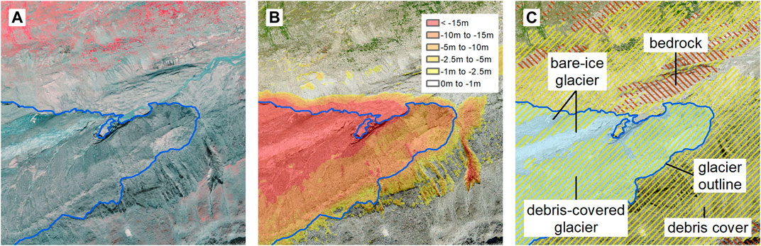
FIGURE 3. The highly debris-covered tongue of Unteraargletscher in the Bernese Oberland as seen on the digital aerial images and used for mapping in 3D-views by swisstopo topographers. The combination of (A) infrared and (B) true color (RGB) combined with swissALTI^3D elevation differences (yellow to red colors) results in (C) swissTLM^3D object classes. The blue line in all panels indicates the swissTLM^3D object class “glacier.”

One of the biggest challenges in glacier mapping is the correct handling of debris-covered glacier parts (e.g. Paul et al., 2013). Delineation of debris-covered glaciers is difficult especially when limited structures (e.g. due to debris cover, shadow, clouds, snow) are present for interpretation in an optical view. As swisstopo performs data evaluation on the basis of aerial images from different years, spectral infrared information, the additional help of surface elevation changes from consecutive swissALTI^3D DEMs and the stereo-metric 3D acquisition technique used to map swissTLM^3D objects, glacier outlines are much easier to define compared to a two-dimensional snapshot only (Weidmann et al., 2019). Moreover, as for the swissTLM^3D not only glaciers are mapped, but many different types of ground cover (e.g. water bodies, debris, rock) that may overlap each other. The object class “debris” (swisstopo, 2021) is implicitly included in the data product. Within reference areas of 625 m² (i.e. 25 × 25 m), swisstopo topographers manually map debris cover on glaciers if its coverage exceeds estimated 80%. The decision however remains to be partly subjective and different degrees of debris coverage, or the thickness of the debris layer are not resolved. In Supplementary Table S1 interactive links providing examples for different aspects of debris-cover classification are given. Hence, an overlay of the object classes “glacier” and “debris” leads to “debris-covered glaciers” (Figure 3).

During production and for updates of the swissTLM^3D, Swiss glaciers are recurrently mapped based on high-resolution data on a long term. After processing the data, swisstopo sends yearly updates of the swissTLM^3D to GLAMOS. The glacier outlines stand out by having a very high level of detail and homogeneity. By 2019, all Swiss glaciers have been mapped according to the new guidelines for the first time, serving as highly valuable basis to produce a new glacier inventory.

Methods

The swissTLM^3D object class “glacier,” here referred to as TLMglac, is the essential baseline data set for the compilation of the new SGI2016. This data set has been digitized by professional swisstopo topographers under the framework of swissTLM^3D as a topographical land-cover data set, but requires further adaptations to meet the needs of a (glaciological) glacier inventory.

Expert Workshop to Define the Requirements for the new SGI2016

After the first complete swissTLM^3D “glacier” object class extract was available, a 1-day glaciological expert workshop was held to examine and discuss the data set. Thereby, the methodological differences between the TLMglac and the previous Swiss Glacier Inventories, some difficulties of the TLMglac for glaciological applications (e.g. glacier definition, seasonal snow, dead-ice bodies) and related required adaptations were discussed. Using all the previous work and data available and discussing specific examples, a common understanding of adaptations to the TLMglac needed from a glaciological point of view was formulated to complete the new SGI2016. The expert workshop revealed that the data set TLMglac is generally mapped on an extremely high level of detail (e.g. shape of the glacier margin digitized at about a scale of 1:5,000–10,000, i.e. with a distance of 0.5–50 m between vertices). However, for a number of locations, entities were found that do not strictly belong to a glacier per definition (e.g. perennial snow patches and avalanche deposits at glacier margins, strongly debris-covered dead-ice bodies, permafrost features in very few cases). These objects have to be removed for the creation of a glacier inventory and are attributed to the object class “snow and dead ice” in the swissTLM^3D. As an outcome of this expert workshop, a reference guideline summarized below was produced to further process and edit the TLMglac data set towards the new SGI2016.

Definition of a Glacier

The polygons of the TLMglac represent the state of glacierization and, in many cases, perennial snow on the latest aerial images used for digitization by the swisstopo topographers. In principle, the glaciers were mapped according to the definition by Cogley et al. (2011), i.e. a glacier is defined as “a perennial mass of ice, and possibly firn and snow […] showing evidence of past or present flow” (Cogley et al., 2011 p. 45). However, especially for very small mapped entities, expert knowledge is required to judge if it is (still) a glacier or not. Leigh et al. (2019) suggested a scoring system to identify and map very small mountain glaciers. For the glacier classification in this study (yes/no) we also put an emphasis on the evidence of flow (crevasses, flow and deformation features, visible ice; cf. Table 4 in Leigh et al., 2019), and cross-checked with aerial images from previous years, to confirm if the size and shape of the mapped entity persists under different conditions. Even though we were able to rely on a guideline and a common understanding among the experts, judging the individual cases remains subjective. However, cross-checks between all experts’ results showed a high correspondence.

Definition of the Minimal Glacier Size

The lower limit of glacier size in the SGI2016 has been defined as 0.01 km² (cf. Kuhn, 1995; Paul et al., 2009). This applies for all polygons with an existing SGI-ID, reflecting the fact that these glacier entities have already been mapped in one of the previous inventories. The threshold for polygons without an already existing SGI-ID (new entities) has arbitrarily been set to 0.025 km² in order to exclude also larger perennial snow patches that had not been recognized as a glacier previously.

Criteria to Identify Features Erroneously Classified as Glacier

The expert workshop revealed that the TLMglac needs to be simplified in some cases and some non-glacier features have to be removed. Considering the TLMglac data set, the previous SGIs, the SWISSIMAGE aerial photographs of the previous 5–10 yr and glaciological knowledge, problematic cases have been recognized and discussed by the glaciologists at the workshop. Features erroneously classified as glacier in the TLMglac can be attributed to the three classes 1) snow, 2) debris, and 3) other, with further subdivision (Table 1; Figure 4 and Supplementary Table S2).

TABLE 1

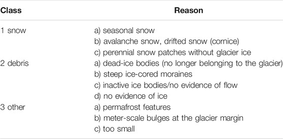
TABLE 1. Classes of the topographical glacier outline data set (TLMglac) that were removed for the SGI2016, including the reason.

FIGURE 4

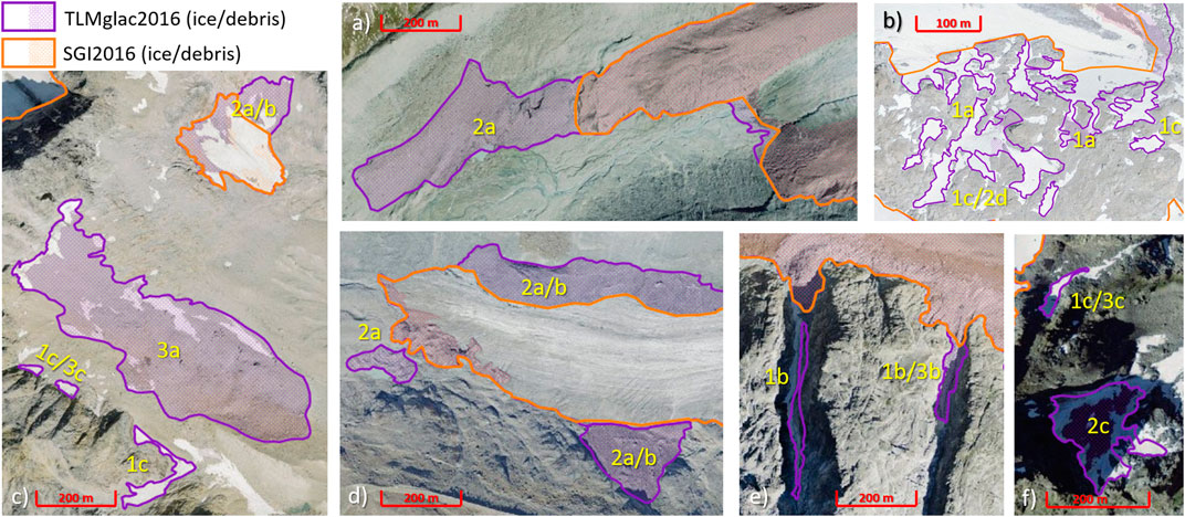
FIGURE 4. Examples of features erroneously mapped as glacier in TLMglac. The numbers and letters indicate the reason according to Table 1 why the purple features (TLMglac) have been removed for the creation of the SGI2016 (orange outlines). A list with links to zoom in at swisstopo’s map browser and investigate the details more closely and in a broader context is available in Supplementary Table S2.

Procedure and Guideline to Create Clipping Masks

The TLMglac does not leave out any potential glacier feature in the Swiss Alps, i.e. we did not find examples where glacier surfaces needed to be added, but in a substantial number of cases parts were removed from the TLMglac to create a glacier inventory fulfilling glaciological criteria. All polygons contained in the TLMglac needed to be cross-checked individually and manually by a glaciologist. We used all available SWISSIMAGE orthophotos (typically available in 3-yr intervals since about 2005) to go back in time. This is crucial, as it supported examination of the polygon mapped as glacier in the TLMglac under different snow depletion conditions, as well as different cast shadows, which is very helpful to confirm if the examined section of the polygon can actually be considered as part of a glacier or not. As a guideline to create clipping masks to cut off erroneously classified features, we used the classes and examples defined in Table 1 (cf. also Figure 4). Additionally, we formulated the following leading questions that help digitizing the clipping masks: 1) Is there some bare glacier ice present? 2) Has seasonal, old, perennial or avalanche snow been mapped? 3) Does potentially debris-covered ice exhibit visible signs of surface dynamics, which can still be attributed to the glacier? 4) Can the glacier geometry be simplified by cutting off (meter-scale) bulges?

Hydrologically-Based Coding System for Unique SGI-IDs

According to the principle already established for the SGI1850, SGI1973 and SGI2010 (Müller et al., 1976; Maisch et al., 2000; Fischer et al., 2014), the unique identifier for single entities within the Swiss Glacier Inventories are the SGI-IDs. The coding system is oriented towards a hydrological, hierarchical classification principle (river levels 0–3) and results in an alphanumeric four-digit code, where every digit refers to a hydrologically-based subdivision of the area (UNESCO, 1970). This results in a unique identifier and allows tracing back all glaciers to their parent-IDs after separation over time (Supplementary Table S3).

From the TLMglac to the new SGI2016: workflow

The workflow to create the new SGI2016 from the TLMglac consists of the following steps:

1. Application of minimal area size threshold (see above).

2. Digitizing clipping masks by experts/glaciologists: The Swiss Alps were divided into five sub-regions that were investigated by at least two of the five experts each to identify features erroneously classified as glacier in TLMglac and to digitize clipping masks according to the defined criteria, procedures and guidelines.

3. Harmonization and generalization: Clipping masks by all experts were merged and homogenized to a single clipping mask that was applied to the TLMglac. The resulting file was generalized using the Douglas-Peucker algorithm (Douglas and Peucker, 1973; QGIS Development Team, 2020) with a tolerance value of 3 m. Finally, the minimal area size threshold from step 1 was applied a second time.

4. Extracting ice divides and clipping debris cover: By extracting the shared polygon boundaries from the generalized TLMglac, the ice divides of the SGI2016 have been derived based on the current swissALTI^3D and attributed with the SGI-IDs of the related glaciers. Ice divides are adjusted to the related inventory based on current ice surface elevation. In a next step, the TLMglac was also used to clip and label the swissTLM^3D object class “debris” in order to get a layer of supraglacial debris cover for each entity of the SGI2016.

5. Glacier inventory parameters: The compilation of the glacier inventory parameters is based on the suggestion by Paul et al. (2009) and the World Glacier Monitoring Service. Supplementary Table S4 provides an overview of all attributes compiled. The unique identifier of the single glacier entities is the SGI-ID and, if not already set from a previous inventory, a new SGI-ID was assigned to the new polygons. The glacier name corresponds to the topographic map sheets (swisstopo, 2020e), if a name is available. The acquisition date of the glacier outline corresponds to the year of acquisition of the aerial images used for glacier mapping (SWISSIMAGE). Surface area is calculated in km² from the polygon(s) and glacier length was measured along an automatically derived center line according to an automated algorithm proposed by Machguth and Huss (2014). Minimum, median, mean and maximum elevation in m a.s.l. as well as mean slope and aspect are based on the up-to-date swissALTI^3D resampled to a spatial resolution of 10 m.

6. Additional data layers: In the course of the preparation of the SGI2016, additional important data layers as location, debris cover, ice divides, center lines and a surface type raster have been produced and are contained in the SGI2016 data package.

Change Assessment and Comparison Between SGI2010 and SGI2016

Due to the fact that glaciers, separating into multiple entities over time, can be traced back to the parent glacier via unique SGI-IDs, a change assessment based on single glacier entities is possible. However, as all SGIs have been compiled based on different source data and somewhat differing methodologies, direct comparison requires caution. The area changes and time difference between SGI1973 and SGI2016 are sufficiently large that the effect of methodological differences is small in relation to the changes. A change assessment based on single glacier entities between SGI1973 and SGI2016 was thus performed. However, as between the SGI2010 and SGI2016 the time difference is relatively small and the methodological differences hamper a direct comparison, we refrained from conducting an automated change assessment based on single glacier entities, but discuss the differences between these inventories in detail below.

Approach to Compare SGI2010 and SGI2016

Comparing SGI2010 with SGI2016 reveals that glacier surface area covered by the latter is slightly higher although strong losses in glacier volume and glacier length were observed between 2010 and 2016 (GLAMOS, 1881-2020; Huss et al., 2015; Zemp et al., 2015). Even though both inventories are based on aerial photographs, the additional data, tools, resources and methodologies used by swisstopo in the frame of producing the TLMglac as the basis for the SGI2016 are beyond the possibilities available at the time of digitizing the SGI2010 (Fischer et al., 2014). It is thus obvious that professional topographers digitizing in 3D, with the help of elaborated guidelines, optical and infrared bands and detailed elevation difference grids from consecutive swissATLI^3D DEMs, achieve a much more detailed cartographic representation of glacier extents in Switzerland. Especially delineating debris-covered glacier parts is much more difficult or even impossible when working only in 2D. The SGI2010 therefore seems to have a tendency to rather underestimate (especially strongly debris-covered) glacier extents. For a direct comparison, the data sets would have to be produced under exactly the same conditions and with the same methodologies.

Reference Data Set SGI2010_ref and Statistical Upscaling

As it is vital for assessing the accuracy of the new SGI2016 in comparison to the SGI2010, and to shed light on the counter-intuitive apparent slight gain in glacier area between 2010 and 2016 – which is clearly suspected to stem from methodological differences – we performed a re-assessment of selected SGI2010 glacier outlines. We thus re-mapped a representative glacier sample drawn from the SGI2010 with exactly the same knowledge and guidelines used to produce the SGI2016. The aim of this experiment is to apply the same glacier definitions as have been used in the SGI2016 to the imagery representing the basis for the SGI2010 and to investigate whether the methodological differences in glacier mapping are able to explain the positive change in overall glacier area.

A sample of 100 glaciers was selected and re-digitized in order to serve as a SGI2010 reference data set (termed SGI2010_ref henceforth). The precondition for the sample was to randomly select glaciers representing all different glacier size classes from all four major catchments. We defined seven area size classes with break values at 0.1; 0.5; 1.0; 2.0, 5.0 and 10 km². The selected sample of 100 glaciers thus represents approximately the distribution in number and area according to the SGI2010, and is representative for the relative distribution of glaciers in the major catchments (numbers of sampled glaciers: Rhine: 35, Rhone: 45, Po: 10, Inn: 10, cf. Figure 1). The objective was to re-digitize SGI2010 outlines, “through the glasses” of the SGI2016 compilation guidelines, especially in relation to debris-covered areas, but with the same resources as for the creation of the SGI2010 (2D orthoimages). The condition for this re-digitization experiment was to not use the SGI2010 outlines, and to only rely on SWISSIMAGE aerial imagery used also by Fischer et al. (2014).

The workload of the re-digitization was distributed among the same five glaciologists that drew the clipping masks to derive SGI2016 outlines from the TLMglac. Every expert digitized the outlines of 32 glaciers randomly distributed in size and region. From the total sample of 100 glaciers, 15 glaciers from all size classes and regions were randomly selected to be digitized by all five experts. The area of the 100 re-digitized glaciers was statistically upscaled to the entire SGI2010 to estimate total glacier surface area. Thereby the differences between the 100 re-digitized and the same 100 SGI2010 glaciers, within the defined seven size classes were used, relying on area fractions of the individual size classes from SGI2010, to derive the upscaled area for 2010. Additionally, the same 100 glaciers have been selected for glacier-individual comparison and change assessment between SGI2010 and SGI2016.

Uncertainty/Accuracy Assessment

Assessing the accuracy of manually digitized glacier outlines is difficult and not straightforward, as it concerns a mapping exercise on aerial or satellite images without in-situ observations (Racoviteanu et al., 2009). Paul et al. (2013) recommend an accuracy assessment based on a “round robin” experiment, i.e. digitization of glacier outlines based on the same imagery by several experts. This was implemented by selecting 15 glaciers spread over all size classes (<0.5 km²: 6 gl.; 0.5–5.0 km²: 6 gl.; >5.0 km²: 3 gl.) and regions, representing bare-ice glaciers, glaciers with substantial supraglacial debris cover, as well as differing conditions of snow depletion. Five experts digitized extents of these glaciers, and the standard deviation of the resulting areas considered as the uncertainty at the glacier-specific level was evaluated. Upscaling the resulting standard deviations to all glaciers, weighted by the respective average glacier area per size class, yields an estimate of the uncertainty in total glacier area at the scale of the Swiss Alps.

Results

The new SGI2016 (data package and key values)

The Swiss Glacier Inventory 2016 provides glacier outlines (areas), supraglacial debris cover, ice divides, center lines and location points of all glaciers in Switzerland referring to the years 2013–2018. Most of the glacier outlines have been mapped based on aerial images acquired between 2015–2017 (75% in number and 87% in area, Table 2), with the center year 2016. The SGI2016 data package is available through 10.18750/inventory.sgi2016.r2020 (GLAMOS, 2020d) and consists of the following files (Figure 5):

• Outline and attribute layer (SGI2016_glaciers.shp): the central inventory file, a polygon layer with SGI-IDs and all inventory parameters (Supplementary Table S4).

• Location layer (SGI2016_locations.shp): a point layer with SGI-IDs, glacier names and x- and y-coordinates. Located manually in the center of accumulation areas, mainly for labelling purposes.

• Debris-cover layer (SGI2016_debris-cover.shp): a polygon layer with SGI-IDs and glacier names of the underlying glaciers, spatial extents of debris cover as well as debris-covered area in km², and year of acquisition.

• Ice-divide layer (SGI2016_icedivides.shp): a polyline layer separating glacier entities along ice divides, with SGI-IDs and glacier names for each side.

• Centre-line layer (SGI2016_centre-lines.shp): a polyline layer providing the longest central flow line per glacier (as well as length in km) and SGI-IDs according to Machguth and Huss (2014).

• Surface type raster (SGI2016_surfacetype_10m.tif): a 10 m resolution raster layer, providing the surface types bare ice and debris-covered ice.

TABLE 2

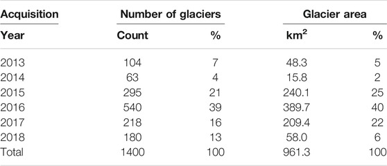
TABLE 2. Glacier distribution in the SGI2016 and corresponding area in relation to the acquisition year of the aerial images used (cf. Figure 1 for spatial distribution).

FIGURE 5

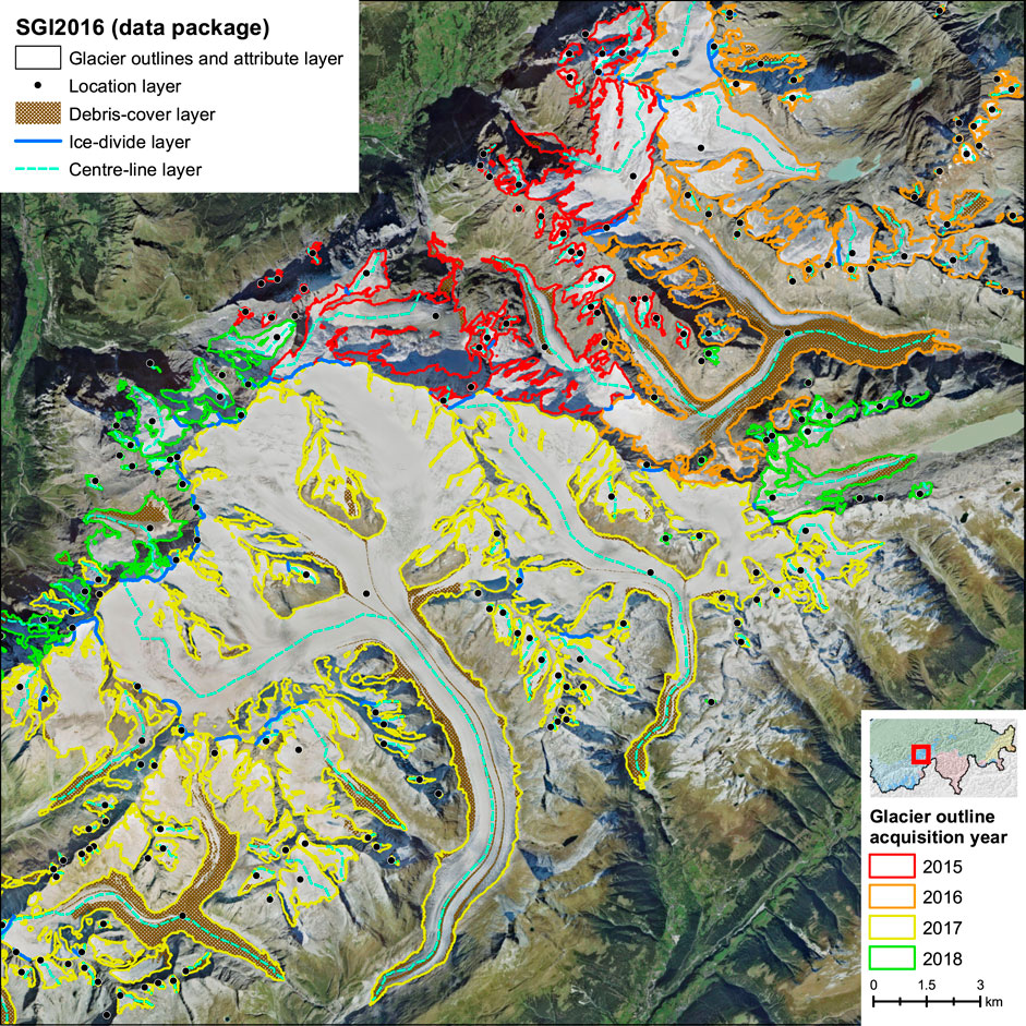
FIGURE 5. Overview on the files provided with the SGI2016 data package in the area of Grosser Aletschgletscher. The glacier outlines are colored according to the acquisition year of the aerial image used for digitizing. Background: SWISSIMAGE orthoimagery composite.

The SGI2016 comprises 1,400 individual glacier entities (unique SGI-IDs) with a total surface area of 961 km² (Tables 2, 3). Most glacier entities are very small (82% of the glaciers are <0.5 km²), but the 46 glaciers with an area larger than 5 km² account for 52% of the total Swiss glacier area. The catchments of Rhine and Rhone show the highest glacierization (in terms of the number of glaciers with 46 and 41%, and in terms of area with 31 and 61%, respectively (Table 3)).

TABLE 3

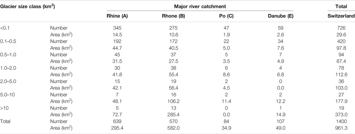
TABLE 3. Number of glaciers and area mapped in the SGI2016, categorized in size classes and major river catchments.

The elevation range of glacier cover in the Swiss Alps spans more than 3,000 m, from the termini of Unterer Grindelwaldgletscher (1,357 m a.s.l.), Oberer Grindelwaldgletscher (1,448 m a.s.l.) and Grosser Aletschgletscher (1,605 m a.s.l.), up to the top of Gornergletscher (4,599 m a.s.l.), Hobärggletscher (4,544 m a.s.l.) and Bisgletscher (4,490 m a.s.l.). Unterer Grindelwaldgletscher and Grosser Aletschgletscher cover an elevation range of more than 2,500 m. Median elevation of glaciers can be taken as a proxy for a balanced-budget equilibrium line altitude (ELA₀) (Braithwaite and Raper, 2009) and strongly varies across the Swiss Alps (Figure 6). In regions with the highest peaks and generally smaller mean annual precipitation (e.g. large parts of the Rhone basin), the median glacier elevation is above 3,000 m a.s.l., but can also be lower than 2,800 m a.s.l. in peripheral regions of the Alps. The overall median elevation of all Swiss glaciers is at 2,938 m a.s.l. (Supplementary Figure S1).

FIGURE 6

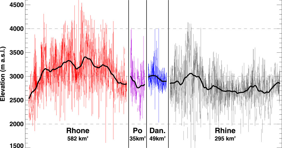
FIGURE 6. Elevation range of all glaciers in the SGI2016, plotted per major river catchment, ordered from west to east (red, B: Rhone; purple, C: Po; blue E: Danube; grey, A: Rhine). Every colored line indicates the elevation range of a single glacier. The bold black line shows a running mean of the median.

Evaluating the glacier sample in three size classes (Supplementary Figure S1) shows that in all four hydrological catchments glaciers larger than 2 km² contribute the majority to the glacierization (Rhone: 55%, Rhine: 77%, Po: 46%, Danube: 55%). For all catchments, the mean slope of the glacier surface is around 20° for glaciers larger than 0.5 km², whereas the size class of very small glaciers (<0.5 km²) exhibits the highest mean slope with almost 30°. The longest glacier of the Swiss Alps is Grosser Aletschgletscher with a total length of 24 km. Long valley glaciers are also found in other catchments, e.g. Unteraargletscher (12 km) in the Rhine basin, or Vadret da Morteratsch (7 km) in the Danube basin.

Debris Cover Within the SGI2016

A new feature of the SGI2016 in comparison to typical glacier inventories (e.g. Gardent et al., 2014; Fischer et al., 2015a; Smiraglia et al., 2015) is the separate debris-cover layer (cf. Figure 5). Although large-scale data sets of supraglacial debris cover are available (Scherler et al., 2018; Herreid and Pellicciotti, 2020), the level of detail of the debris-cover product included in the SGI2016 paves the way for further process-based studies on feedback effects between debris cover and glacier evolution. The high-resolution aerial imagery used for mapping is very distinct, e.g. showing the partly only 10 m wide famous middle moraines of Grosser Aletschgletscher from their origin at the glacier confluences of tributaries at Konkordiaplatz to the glacier terminus (Figure 5). In total, 11% (104.0 km²) of the total Swiss glacier area were debris-covered in 2016. The share of debris-covered ice surfaces is similar in the Rhone, Rhine and Danube catchments (10–11%), but is higher (16%) in the Po catchment (Table 4). Given the relatively limited glacierization in the Po catchment (Table 3), interpreting the higher ratio of debris-covered ice is speculative but might be related to the relatively low elevation of glaciers (Figure 6) and the generally high surface slopes of the surrounding terrain favoring enhanced erosion rates (e.g. Benn et al., 2012; Westoby et al., 2020). Ranking all individual Swiss glaciers according to their absolute debris-covered area indicates that only five glaciers account for a quarter of the overall area with supraglacial debris (Figure 7). For the glaciers with considerable debris-covered surfaces, three types can be distinguished: 1) Large glaciers with a completely debris-covered tongue (e.g. Unteraar, Oberaletsch, Zmutt, Zinal). The typical share of debris-covered ice for this case is around 30%. 2) Very large glaciers with a moderate share of debris (less than 10%) which still accounts for a relevant absolute area due to the sheer size of the glaciers (e.g. Grosser Aletsch, Gorner, Fiescher). 3) Small to medium-sized glaciers with a very high debris-to-bare-ice ratio (50% or more, e.g. Tsessette, Albigna, Griess, Gavirolas).

TABLE 4

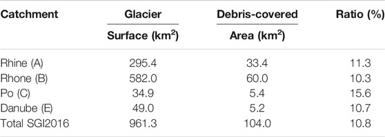
TABLE 4. Area and ratio of debris-covered glacier surface per main hydrological catchment and for the entire inventory.

FIGURE 7

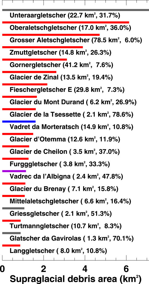
FIGURE 7. SGI2016 glaciers ranked according to their absolute area with supraglacial debris. For each glacier, the total area and the share of debris-cover is stated. Colors refer to the main hydrological catchment (grey: Rhine, red: Rhone; purple: Po; blue: Danube).

Analyzing the dependencies between topographic parameters (mean slope, glacier length, median elevation) and debris-cover fraction reveals that short (<0.5 km) glaciers with a moderate mean slope (20–30°) and a low median elevation (<2,600 m a.s.l.) tend to have high debris-cover fractions (Figure 8). Morphological processes that are closely linked to topography and that favor high debris coverage can most likely explain these dependencies (e.g. Salerno et al., 2017; Westoby et al., 2020). Whereas supraglacial debris is less likely to accumulate on very steep glaciers, the area around gently-sloping glaciers is less prone to erosion. Highest debris-cover fractions are thus found for glaciers with medium average slopes (Figure 8A). Although some long glaciers exhibit important absolute debris-covered areas (Figure 7), the average share of debris on relatively large and long valley glaciers is typically reduced in comparison to small and short glaciers (Figure 8B). Short glaciers often are located in mountain cirques surrounded by steep rock walls that favor accumulation of debris on the ice. The relation between relative debris coverage and median elevation is very clear: Whereas glaciers at high elevation have small average debris fractions, glaciers at low elevation are strongly debris-covered (Figure 8C). This is likely related to the melt reduction exerted by debris, permitting glacier ice to be present at lower elevation (Nicholson and Benn, 2006; Brun et al., 2019). On the other hand, glaciers at low elevation are characterized by higher snow accumulation rates and, thus, higher mass balance gradients and, thus, an enhanced erosional potential.

FIGURE 8

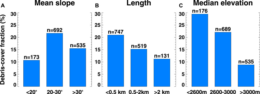
FIGURE 8. Dependence of the arithmetic mean of the glaciers’ debris-cover fraction on classes of topographic parameters: (A) mean surface slope, (B) glacier length, and (C) median elevation. The number of glaciers per class (n) is given.

The hypsometric distribution of glacier surface and debris-cover in Figure 9 reveals that glacier areas below an elevation of 2,500 m a.s.l. are highly debris-covered in all catchments with a fraction ranging from around 40% up to 100%. Due to the higher peaks and the inner alpine climate in the Rhone catchment, the median elevation of these glaciers is generally higher, which also leads to a higher debris-cover fraction at elevations of up to 3,000 m a.s.l. (Figure 9).

FIGURE 9

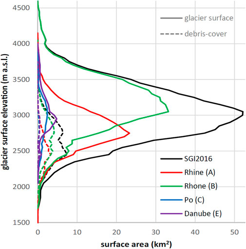
FIGURE 9. Glacier surface and debris-cover distribution in hypsometric bands of 50 m for the four major river catchments and entire Swiss Alps.

Change Assessment SGI1973 – SGI2016

The 2,732 mapped glacier entities in the SGI1973 cover an area of 1,311 km², and the 1,400 individual glaciers in the SGI2016 cover an area of 961 km². This corresponds to an overall area change of –350 km², –26.7% or –0.6% a⁻¹ between 1973 and 2016. As the glaciers in the SGI2016 are linked to the SGI1973 via unique IDs, dissolving the 1,400 SGI2016 glacier IDs based on the SGI1973 parent-IDs results in 1,335 individual IDs, from which 1,330 could be joined to a corresponding parent-ID in the SGI1973. Only five glaciers in the Central Swiss Alps covering a total area of 0.14 km² could not be related to a glacier mapped in SGI1973, as at these locations no glaciers were mapped in the SGI1973. From the SGI1973 to the SGI2016, 1,402 SGI-IDs with a total area of 58 km² disappeared completely and are not anymore relevant for a direct change assessment based on individual glacier IDs. All these entities were smaller than 0.5 km² and over 90% of them were smaller than 0.1 km² in 1973. The catchment-wise loss in area was 20.5 km² (A: Rhine), 23.4 km² (B: Rhone), 7.3 km² (C: Po), 6.9 km² (E: Inn), and regarding the total glacier count correspond to 40% (A), 32% (B), 12% (C), 16% (E) of the glaciers. The remaining 1,330 glacier entities from the SGI1973 with matching glacier units in the SGI2016 covered 1,253 km² in 1973.

The strongest relative change in glacier area between 1973 and 2016 occurred in the Po catchment (–36.4%). Relative area change was least negative in the Rhone basin (–18.7%, Figure 10A). These regional differences can be attributed to the glacier size distribution. Relative area changes are largest for small glaciers (Figure 10B) that are predominant in the Po catchment, whereas the Rhone basin includes the largest glaciers with smaller relative area changes (despite of large absolute area changes; e.g. the two largest glaciers: Grosser Aletschgletscher –8.13 km²/–9.4%, Gornergletscher –5.38 km²/–9.0%). A very clear dependence of relative area changes on classes of surface slope is evident (Figure 10C): the steeper the glacier on average, the larger the relative area change. This finding corresponds to observations of glacier mass balances (e.g. Fischer et al., 2015b; Brun et al., 2019). Small glaciers exhibit large relative area changes, and they are generally steeper than large glaciers. Furthermore, steep glaciers are thinner and will thus respond more quickly to a change in climate by adapting their length and thus area. Relative area changes are similar for all aspect classes (Figure 10D). South-facing glaciers experienced smaller area changes. This is only counter-intuitive at first glance because south-facing glaciers are situated at higher elevation (due to enhanced solar radiation input), where they are less sensitive to changes in air temperature. Median elevation and relative area changes also show a clear relation, with low-elevation glaciers experiencing the largest changes and glaciers at high elevation the most moderate ones (Figure 10E). The dependency of relative area change on present (SGI2016) debris-cover fraction is less clear, but there is a tendency that glaciers with a high share of supraglacial debris show larger area changes (Figure 10F). This observation is not intuitive, because (continuous and thick) debris cover is known to strongly reduce melt rates (e.g. Anderson, 2000; Banerjee and Shankar, 2013). However, due to debris coverage, these glaciers extend to lower elevation where they are more sensitive to climate forcing, and they generally have a smaller accumulation area that will be completely lost with only a limited rise in the equilibrium line altitude. A presently high share of supraglacial debris might also be a result of strong retreat over the last decade. Our observations indicate that the area of debris-covered glaciers responds in a similar way to climate change as for bare-ice glaciers.

FIGURE 10

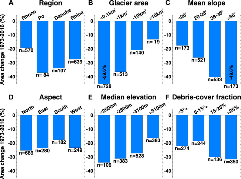
FIGURE 10. Arithmetic mean of glacier-specific relative area changes 1973–2016 according to (A) the major catchment, and classes of (B) glacier area, (C) mean surface slope, (D) principal surface aspect, (E) median elevation, and (F) debris-cover fraction according to the SGI2016. The number of glaciers per class (n) is given.

Discussion

Re-assessment of the Overall Area Loss SGI2010 – SGI2016

The total glacier area of the SGI2010 amounts to 944 ± 24 km² for the year 2010 (Fischer et al., 2014), whereas the new product SGI2016 reports an area of 961 ± 22 km² for Switzerland. In light of major glacier mass losses observed in the Alps between 2010 and 2016 (e.g. GLAMOS, 1881-2020; Beniston et al., 2018; WGMS, 2020), this increase in glacier area by 2% is counter-intuitive, and is suspected to stem from methodological differences. To investigate these differences, we performed a re-digitization experiment for 100 glaciers based on the same imagery as had been used for the SGI2010 but with the approaches and the definitions elaborated for the compilation of the SGI2016. For the 100 selected glaciers, the SGI2010 reports an area of 196.3 km², and the SGI2016 196.7 km². An area of 205.2 km² is found for the re-digitized glacier sample SGI2010_ref (Table 5), thus indicating an actual area change of –4.2% between 2010 and 2016.

TABLE 5

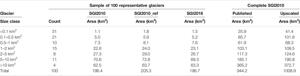
TABLE 5. Results of the SGI2010 re-digitization experiment and upscaling to all Swiss glaciers.

For re-digitizing the sample of 100 selected glaciers for the SGI2010_ref it was not possible to rely on exactly the same methodologies and resources as for the production of the SGI2016 as various source data (e.g. high-resolution DEM differences) used for the compilation of the SGI2016 were not yet available when the SGI2010 was produced. However, applying the same glacier definition as for the SGI2016 for glacier mapping in the SGI2010 results in generally larger glacier areas, particularly for highly debris-covered areas (Figure 11). Re-digitized outlines of accumulation areas and bare-ice areas however correspond very well with the SGI2010, indicating that the differences are driven by the recognition of debris-covered ice as part of the inventory. Comparing the 100 glaciers from the re-digitized SGI2010_ref with the corresponding outlines from the SGI2010 reveals that the area of 90 glaciers is larger in the SGI2010_ref, and for ten glaciers the area is equal or smaller in the re-assessment. In absolute values, the area changes per individual glaciers are rather small, with a minimum of –0.03 km² (SGI2010 area is larger than in the re-assessment) to a maximum of +0.71 km², with a median of +0.03 km² (+7%). The re-assessment indicates more than 100% greater area for ten glaciers smaller than 0.5 km² in the SGI2010. These glaciers sum up to a small absolute area gain (+0.44 km²), but it was observed that considerable interpretation differences occur for small and very small glaciers (Figure 11A).

FIGURE 11

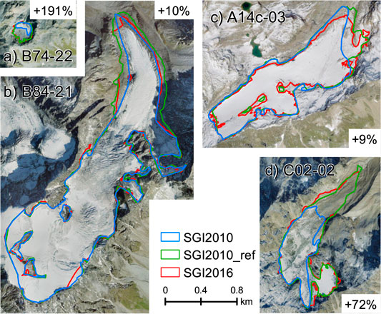
FIGURE 11. Four examples of re-assessed glacier outlines of the SGI2010 based on the re-digitization experiment using the same source imagery, but with the approaches and definitions used for the SGI2016 (Supplementary Table S5). The re-digitized outlines are labelled SGI2010_ref and area differences relative to the original data set (SGI2010) are given in all panels. (A) Glacier d’Orchère (area A₂₀₁₀ = 0.01 km²), (B) Glacier de Valsorey, (A₂₀₁₀ = 1.88 km²), (C) Fanellgletscher (A₂₀₁₀ = 0.83 km²), (D) Bodmergletscher (A₂₀₁₀ = 0.33 km²). The background imagery corresponds to the SWISSIMAGE orthophotos used as source data for the compilation of the SGI2010 and the codes represent the unique SGI-IDs.

For upscaling the results of the re-assessment experiment to all 1,441 glaciers of the SGI2010, we use the relative area change per size class. Based on the re-assessment we find an upscaled total glacier surface area at the time of the SGI2010 of 1,009 km² (Table 5). From this analysis we conclude that, if the SGI2010 would have been digitized with the definitions, rules, knowhow and source data as used for the compilation of the SGI2016, the total glacier area would have been bigger (+64.7 km², +6.9%). In comparison to the SGI2016, the re-assessed area of the SGI2010 corresponds to an absolute area change of –47.6 km² and a relative change of –4.7% between SGI2010 and SGI2016, implying an annual area change of –0.8% (Table 6). This relative area loss is similar to the –0.7% a⁻¹ reported for 1973 to 2010 (Fischer et al., 2014), but is smaller than the values of –1.1% a⁻¹ to –1.3% a⁻¹ found for the entire Alps between 2003 and 2015/16 (Paul et al., 2020) and the value of –1.4% a⁻¹ for the Swiss Alps from 1985 to 1998/99 (Paul et al., 2004).

TABLE 6

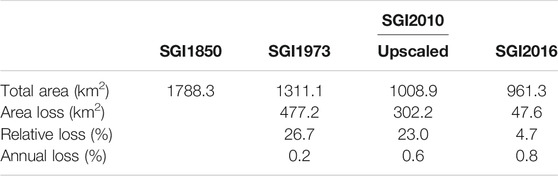
TABLE 6. Absolute and relative area loss over time according to the SGI’s.

Accuracy Assessment

In order to quantify the overall uncertainty in glacier area digitized based on the available high-resolution imagery, we analyze independent results of the “round robin” experiment on multiple digitization of glaciers by five experts. Due to the quality and resolution of the SWISSIMAGE orthoimagery and the clearly defined rules and guidelines for glacier mapping elaborated for the SGI2016, all experts generally delineated the glacier outlines highly consistently. Especially for bare-ice glaciers, where the glacier ice directly meets bare bedrock, digitized glacier margins lie in general within 2–10 m of horizontal distance. Only in some exceptional cases they differed by up to 100 m because of in-/excluding small branches (Figure 12A, cf. southern spike) or due to snow cover or clouds (Figure 12C). For debris-covered glacier ice on sedimentary beds the deviations of the outlines are often somewhat larger (5–50 m), i.e. the different interpretations of the glacier boundaries do not agree everywhere, but in most cases match well (Figure 12D). The largest variability between digitized outlines has been found for a very small glacier in a shadowed, snow-covered north face (Figure 12B) with a standard deviation of inferred glacier area of 23.8%. For all other of the 15 analyzed glaciers covering different size classes and characteristics, the standard deviation lies between 0.3 and 7.1% (Supplementary Table S6). Upscaling these standard deviations according to the area fraction in three size classes (Supplementary Table S7), we find an uncertainty in total glacier area of ± 2.3%, or ± 21.7 km² for the SGI2016. When comparing these values with the studies of Paul et al. (2013) and Fischer et al. (2014) who performed similar digitization experiments, the results correspond well, but tend to be somewhat smaller, which is attributed to the higher resolution of the available imagery and the consistent application of defined rules and guidelines for glacier mapping by all experts. Higher relative area uncertainties with decreasing glacier size (e.g. Paul et al., 2003; Fischer et al., 2014) could also be observed and confirmed.

FIGURE 12

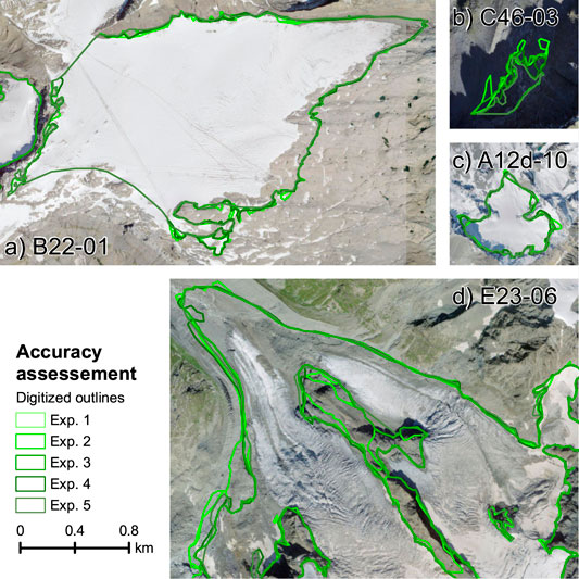
FIGURE 12. Four examples of the digitization experiment for the accuracy assessment of the SGI2016 with outlines digitized by the five experts. The background imagery corresponds to the SWISSIMAGE orthophotos used as source data for the compilation of glacier outlines and the codes represent the unique SGI-IDs.

SGI2016 and the Previous Inventories

All previous glacier inventories for Switzerland, also available via GLIMS, have been produced with the best data sources, methodology and knowledge available at the time. Since all inventories are subject to uncertainties and have been established using different methodologies, a direct change assessment at the scale of individual glaciers is difficult. However, aggregated results for the major river catchments, the glacier size classes or the glacierization of the entire Swiss Alps can be compared (Supplementary Table S8). The area distribution per size class is very similar in all inventories. Throughout all inventories the glaciers smaller than 0.5 km² contribute 12–16% to the total glacier area and the glaciers larger than 10 km² 35–39%.

Figure 2 and Supplementary Figure S2 provide a comparison of the outlines for the Swiss glaciers available via GLIMS and the new SGI2016 and reveal the different characteristics of the inventories. For glacier ice without debris coverage, the retreat is easily recognizable and measurable via the surface area (Figure 2). As soon as the glaciers are debris-covered, the time component of the inventories is of secondary importance, but acquisition techniques become more relevant. SGI1973, SGI2010 and SGI2016 that have been manually compiled based on aerial orthophotos contain more debris-covered glacier surfaces due to a higher resolution of the base data compared to the inventories Alps-2003, Alps-2015 and SGI2010 that were compiled using semi-automatic mapping with satellite imagery (Supplementary Figure S2).

The Alps-2015 inventory (Paul et al., 2020) reports a glacier area of 890 km² for Switzerland which is significantly smaller than our results for the quasi-simultaneous new SGI2016 (961 km²). The difference of about 7% can probably be assigned to methodological differences and the much higher level of detail in glacier mapping of the SGI2016. The differences can mostly be attributed to the mapping of debris-covered areas of large glaciers (Supplementary Figure S2). For example, the mapped surface areas for the highly debris-covered Unteraargletscher, Oberaletschgletscher and Glacier de Zinal (Figure 7) are 8.8, 7.8 and 7.9% larger in the SGI2016 compared to the Alps-2015, accounting for 4.1 km² in total.

The swissTLM^3D object classes “glacier” and “debris” are digitized independently. Debris is mapped when the coverage exceeds 80% in an area of 25 × 25 m. However, as recognizable on the interactive maps (cf. links in Supplementary Table S1), the decisions taken during mapping may differ between regions as the classification is still partly based on subjective criteria. Further improvement is foreseen as the object classes are regularly updated feeding into a next inventory. We assume that glacier outlines of debris-covered glaciers were mapped more accurately in our new inventory due to the imagery’s spatial resolution, which was 20–40 times higher in comparison to Sentinel-2 imagery as used in the Alps-2015 inventory. In addition, mapping in 3D and the consideration of surface elevation differences adds a considerable benefit for more accurately detecting dead-ice bodies and debris-covered parts of glaciers. In contrast, the Alps-2015 data set contains about 30% more individual glacier entities than the SGI2016. However, this number is difficult to be interpreted, as some glacier polygons in the SGI2016 have the same SGI-ID because they belong to the same parent glacier and are therefore counted as one entity.

The comparison of the two latest glacier inventories for the Swiss Alps (Alps-2015, Paul et al., 2020; SGI2016, this study) reveals the substantial challenges in mapping highly debris-covered glacier surfaces only based on 2D snapshots. With regard to the worldwide glacier retreat, the increase of supraglacial debris coverage and the disintegration of glaciers, our assessment indicates that additional data sources (e.g. elevation differences) and tools (e.g. 3D-mapping, consideration of surface velocities) are key to better constrain glacier margins in debris-covered areas.

Today, satellite-based DEMs with a vertical accuracy and ground resolution comparable to the swissALTI^3D data set used for the SGI2016 are available and provide high-resolution terrain information over glacierized areas worldwide (e.g. Berthier et al., 2014; Pandey et al., 2017). Elevation differences derived from consecutive high-resolution DEMs, for instance from sub-meter Pléiades stereo images or TerraSAR-X TanDEM-X data based on radar interferometry techniques, may therefore have the potential to foster more accurate glacier mapping over (highly) debris-covered glaciers worldwide, and to improve (and minimize the amount of time needed for) manual correction of automatically generated glacier outlines based on glacier mapping techniques using satellite data and band ratio thresholds.

Comparing the total glacier surface area only of the SGIs derived from maps and aerial images by manual digitizing (Figure 2; category (a)), and substituting the reported SGI2010 total area by the upscaled value from this study, reveals relative area change rates that increase over time, from –0.2% a⁻¹ (1850–1973), to –0.6% a⁻¹ (1973–2010) to –0.8% a⁻¹ (2010–2016) (Table 6). The first two periods show an acceleration of area-change rates although the length of the time intervals strongly differs. This acceleration is consistent with observed long-term changes in mass balance in the European Alps (e.g. Beniston et al., 2018). The period 2010–2016 seems to indicate a further acceleration in glacier area change that is also highlighted by Paul et al. (2020) and agrees with monitoring results. Nevertheless, the signal has to be interpreted with care as the period is short and might be influenced by uncertainties in the inventories and short-term meteorological variability.

As shown before, estimating the uncertainties in the SGI2010 and correcting the total area according to a consistent glacier definition is possible due to the temporal proximity of the inventory to the SGI2016 and the available baseline data. The uncertainties in the older inventories SGI1850 and SGI1973 are not assessed here, but they probably tend to be higher due to the applied methodologies in mapping these outlines. However, the time period for a change assessment with the SGI2016 glacier extent is sufficiently large that the uncertainties may play a minor role and likely mapping debris-covered glaciers was not the same troublesome issue as today.

Cooperation Between Swisstopo an GLAMOS

The production of the SGI2016 was only possible due to the close exchange between the topographers at swisstopo and the glaciologists at GLAMOS over the past years. It was self-evident to embed the production of the next Swiss Glacier Inventories into already existing products of swisstopo. The constraint to regularly produce an updated glacier inventory required both institutions to boost the cooperation and to start mutual learning. This process led to adapted and adjusted production guidelines on both sides. Meetings and workshops helped to understand the different professional backgrounds of topographers and glaciologists, to find common solutions for specific problems related to glacier mapping, and finally to derive a state-of-the-art glaciological data set. The SGI2016 influences the coming swissTLM^3D releases and will streamline the production of future Swiss Glacier Inventories. The SGI2016 is the first step towards a consistent and accurate data product of repeated glacier inventories in 6-yr time intervals that promises a high comparability for individual glaciers and glacier samples, secured due to the integration into long-term projects on both sides.

Conclusion

We presented the new Swiss Glacier Inventory SGI2016 that has been acquired based on high-resolution aerial imagery (with a resolution of 0.25–0.50 m) and digital elevation models (swissALTI^3D, with 2 m resolution) in cooperation with the Federal Office of Topography (swisstopo) and Glacier Monitoring in Switzerland (GLAMOS), bringing together topographical and glaciological knowledge. We describe and define the process, workflow and required glaciological adaptations to compile a highly detailed glacier inventory based on the digital Swiss Topographic Landscape Model (swissTLM^3D) The resulting high-resolution glacier inventory will support process studies and model validation/calibration for glaciers in the Swiss Alps. However, the complete process of compiling the inventory strongly relies on the high detail of data sets available in Switzerland and may not be directly applicable in other mountain ranges.

The SGI2016 provides glacier outlines (area), supraglacial debris cover, ice divides, center lines and location points of all glaciers in Switzerland referring to the years 2013–2018, whereas most of the glacier outlines have been mapped based on aerial images acquired between 2015 and 2017 (75% in number and 87% in area), with the center year 2016. Our data set contains 1,400 individual glacier entities with a total glacier surface area of 961 ± 22 km² (whereof 11%, or 104 km² are debris-covered) and constitutes the so far most detailed cartographic representation of the glacier extent in Switzerland. The data package comprises an individual layer of debris-covered glacier area. Analyzing the dependencies between topographic parameters and debris-cover fraction on the basis of individual glaciers reveals that (small and) short glaciers with a moderate mean slope and glaciers with a low median elevation tend to be strongly debris-covered.

To be able to track and assess glacier changes between the previous Swiss Glacier Inventories and future releases to come, the coding system of SGI-IDs introduced in the 1970s (Müller et al., 1976; Maisch et al., 2000) was pursued. A change assessment between the SGI1973 and SGI2016 based on individual glacier entities confirms the largest relative area changes for small glaciers and for low-elevation glaciers, whereas the largest glaciers show small relative area changes, though large absolute changes. The analysis further indicates a tendency for glaciers with a high share of supraglacial debris to show larger relative area changes.

Despite an observed strong glacier volume loss between 2010 and 2016 (e.g. Beniston et al., 2018), the total glacier surface area of the SGI2016 is somewhat larger than reported in the last published Swiss Glacier Inventory (SGI2010, Fischer et al., 2014). Even though both inventories were created based on swisstopo aerial photographs, the additional data, tools, resources and methodologies used by the professional topographers digitizing glacier outlines in 3D for the SGI2016, and subsequent adaptations and corrections carried out by glaciologists, are able to explain the counter-intuitive difference between SGI2010 and SGI2016. Due to methodological differences and the time interval of only 6 yr that is too small to make a reasonable comparison within the inherent uncertainties of glacier inventories, a direct change assessment between SGI2010 and SGI2016 is not meaningful. However an experiment where a representative glacier sample of the SGI2010 was re-assessed based on the approaches of the SGI2016 led to an upscaled total glacier surface area of 1,009 km² for the Swiss Alps around 2010. A comparison to the latest glacier inventory of the (Swiss) Alps based on Sentinel-2 satellite imagery, band rationing and manual corrections (Paul et al., 2020) highlights the usefulness of additional data (e.g. elevation differences) and 3D-mapping tools as key elements to better constrain glaciers extents in highly debris-covered areas. Consequently, mapped glacier area in the SGI2016 based on high-resolution aerial orthoimages is about 7% larger than according to satellite data for the same time.

As swisstopo data products are and will be regularly updated, the SGI2016 is the first step towards a consistent and high-quality data product of repeated glacier inventories in 6-yr time steps providing a high comparability for individual glaciers and glacier samples. The fruitful cooperation between swisstopo and GLAMOS will thus continue and result in consistent future inventories for Swiss glaciers.

Data Availability Statement

The datasets presented in this study can be found on the GLAMOS online repository, https://doi.glamos.ch/data/inventory/inventory_sgi2016_r2020.html.

Author Contributions

AL designed and led the study and coordinated works of co-authors. AL and MH wrote the manuscript and elaborated most figures. AL, MH, EH, AB, and MF acted as glaciologist-experts, digitized clipping masks and the SGI2010_ref glacier sample. EH contributed Figure 3, was responsible for all steps of the compilation of the SGI2016 data package, and stored the inventory in the database that was set up by YW and EH. HB and ES are responsible for the swissTLM^3D and provided the swisstopo data. All co-authors contributed to the manuscript and helped with the completion of the paper.

Conflict of Interest

The authors declare that the research was conducted in the absence of any commercial or financial relationships that could be construed as a potential conflict of interest.

Publisher’s Note

All claims expressed in this article are solely those of the authors and do not necessarily represent those of their affiliated organizations, or those of the publisher, the editors and the reviewers. Any product that may be evaluated in this article, or claim that may be made by its manufacturer, is not guaranteed or endorsed by the publisher.

Acknowledgments

This study was conducted in the frame of Glacier Monitoring Switzerland (GLAMOS). The program is supported by the Federal Office for the Environment, MeteoSwiss in the frame of the Global Climate Observing System (GCOS) Switzerland and the Swiss Academy of Sciences (SCNAT). Helpful comments by the reviewers Qiao Liu and Andrea Fischer as well as the scientific editor Alun Hubbard contributed to the final version of the paper.

Supplementary Material

The Supplementary Material for this article can be found online at: https://www.frontiersin.org/articles/10.3389/feart.2021.704189/full#supplementary-material

References

Abermann, J., Fischer, A., Lambrecht, A., and Geist, T. (2010). On the Potential of Very High-Resolution Repeat DEMs in Glacial and Periglacial Environments. The Cryosphere 4, 53–65. doi:10.5194/tc-4-53-2010

CrossRef Full Text | Google Scholar

Anderson, R. S. (2000). A Model of Ablation-Dominated Medial Moraines and the Generation of Debris-Mantled Glacier Snouts. J. Glaciol. 46, 459–469. doi:10.3189/172756500781833025

CrossRef Full Text | Google Scholar

Andreassen, L. M., Paul, F., Kääb, A., and Hausberg, J. E. (2008). Landsat-derived Glacier Inventory for Jotunheimen, Norway, and Deduced Glacier Changes Since the 1930s. The Cryosphere 2, 131–145. doi:10.5194/tc-2-131-2008

CrossRef Full Text | Google Scholar

Banerjee, A., and Shankar, R. (2013). On the Response of Himalayan Glaciers to Climate Change. J. Glaciol. 59, 480–490. doi:10.3189/2013JoG12J130

CrossRef Full Text | Google Scholar

Barcaza, G., Nussbaumer, S. U., Tapia, G., Valdés, J., García, J.-L., Videla, Y., et al. (2017). Glacier Inventory and Recent Glacier Variations in the Andes of Chile, South America. Ann. Glaciol. 58, 166–180. doi:10.1017/aog.2017.28

CrossRef Full Text | Google Scholar

Beniston, M., Farinotti, D., Stoffel, M., Andreassen, L. M., Coppola, E., Eckert, N., et al. (2018). The European Mountain Cryosphere: A Review of its Current State, Trends, and Future Challenges. The Cryosphere 12, 759–794. doi:10.5194/tc-12-759-2018

CrossRef Full Text | Google Scholar

Benn, D. I., Bolch, T., Hands, K., Gulley, J., Luckman, A., Nicholson, L. I., et al. (2012). Response of Debris-Covered Glaciers in the Mount Everest Region to Recent Warming, and Implications for Outburst Flood Hazards. Earth-Science Rev. 114, 156–174. doi:10.1016/j.earscirev.2012.03.008

CrossRef Full Text | Google Scholar

Berthier, E., Vincent, C., Magnússon, E., Gunnlaugsson, Á. Þ., Pitte, P., Le Meur, E., et al. (2014). Glacier Topography and Elevation Changes Derived from Pléiades Sub-meter Stereo Images. The Cryosphere 8, 2275–2291. doi:10.5194/tc-8-2275-2014

CrossRef Full Text | Google Scholar

Bliss, A., Hock, R., and Radić, V. (2014). Global Response of Glacier Runoff to Twenty-First Century Climate Change. J. Geophys. Res. Earth Surf. 119, 717–730. doi:10.1002/2013JF002931

CrossRef Full Text | Google Scholar

Bolch, T., Menounos, B., and Wheate, R. (2010). Landsat-based Inventory of Glaciers in Western Canada, 1985-2005. Remote Sensing Environ. 114, 127–137. doi:10.1016/j.rse.2009.08.015

CrossRef Full Text | Google Scholar

Braithwaite, R. J., and Raper, S. C. B. (2009). Estimating Equilibrium-Line Altitude (ELA) from Glacier Inventory Data. Ann. Glaciol. 50, 127–132. doi:10.3189/172756410790595930

CrossRef Full Text | Google Scholar

Brun, F., Wagnon, P., Berthier, E., Jomelli, V., Maharjan, S. B., Shrestha, F., et al. (2019). Heterogeneous Influence of Glacier Morphology on the Mass Balance Variability in High Mountain Asia. J. Geophys. Res. Earth Surf. 124, 1331–1345. doi:10.1029/2018JF004838

CrossRef Full Text | Google Scholar

Carrivick, J. L., James, W. H. M., Grimes, M., Sutherland, J. L., and Lorrey, A. M. (2020). Ice Thickness and Volume Changes Across the Southern Alps, New Zealand, From the Little Ice Age to Present. Sci. Rep. 10, 13392. doi:10.1038/s41598-020-70276-8

PubMed Abstract | CrossRef Full Text | Google Scholar

Cogley, J. G., Hock, R., Rasmussen, L. A., Arendt, A. A., Bauder, A., Braithwaite, R. J., et al. (2011). Glossary of Glacier Mass Balance and Related Terms. Paris: UNESCO-IHP. Available at: http://unesdoc.unesco.org/images/0019/001925/192525E.pdf.

Google Scholar

Douglas, D. H., and Peucker, T. K. (1973). Algorithms for the Reduction of the Number of Points Required to Represent a Digitized Line or its Caricature. Cartographica 10, 112–122. doi:10.3138/fm57-6770-u75u-7727

CrossRef Full Text | Google Scholar

Earl, L., and Gardner, A. (2016). A Satellite-Derived Glacier Inventory for North Asia. Ann. Glaciol. 57, 50–60. doi:10.3189/2016AoG71A008

CrossRef Full Text | Google Scholar

EAW (1954). Planimetrierung der Gletscher, Flächenstatistik (Schweiz und ausländisches Territorium bearbeitet auf “Landeskarte”). Eidgenössisches Amt für Wasserwirtschaft.

Google Scholar

Eis, J., Maussion, F., and Marzeion, B. (2019). Initialization of a Global Glacier Model Based on Present-Day Glacier Geometry and Past Climate Information: An Ensemble Approach. The Cryosphere 13, 3317–3335. doi:10.5194/tc-13-3317-2019

CrossRef Full Text | Google Scholar

Fischer, A., Seiser, B., Stocker Waldhuber, M., Mitterer, C., and Abermann, J. (2015a). Tracing Glacier Changes in Austria from the Little Ice Age to the Present Using a Lidar-Based High-Resolution Glacier Inventory in Austria. The Cryosphere 9, 753–766. doi:10.5194/tc-9-753-2015

CrossRef Full Text | Google Scholar

Fischer, M., Huss, M., Barboux, C., and Hoelzle, M. (2014). The New Swiss Glacier Inventory SGI2010: Relevance of Using High-Resolution Source Data in Areas Dominated by Very Small Glaciers. Arctic, Antarctic, Alpine Res. 46, 933–945. doi:10.1657/1938-4246-46.4.933

CrossRef Full Text | Google Scholar

Fischer, M., Huss, M., and Hoelzle, M. (2015b). Surface Elevation and Mass Changes of All Swiss Glaciers 1980-2010. The Cryosphere 9, 525–540. doi:10.5194/tc-9-525-2015

CrossRef Full Text | Google Scholar

Freudiger, D., Mennekes, D., Seibert, J., and Weiler, M. (2018). Historical Glacier Outlines from Digitized Topographic Maps of the Swiss Alps. Earth Syst. Sci. Data 10, 805–814. doi:10.5194/essd-10-805-2018

CrossRef Full Text | Google Scholar

Frey, H., Paul, F., and Strozzi, T. (2012). Compilation of a Glacier Inventory for the Western Himalayas from Satellite Data: Methods, Challenges, and Results. Remote Sensing Environ. 124, 832–843. doi:10.1016/j.rse.2012.06.020

CrossRef Full Text | Google Scholar

Gardent, M., Rabatel, A., Dedieu, J.-P., and Deline, P. (2014). Multitemporal Glacier Inventory of the French Alps from the Late 1960s to the Late 2000s. Glob. Planet. Change 120, 24–37. doi:10.1016/j.gloplacha.2014.05.004

CrossRef Full Text | Google Scholar

GLAMOS (2020a). Swiss Glacier Inventory 1850. doi:10.18750/inventory.sgi1850.r1992

CrossRef Full Text | Google Scholar

GLAMOS (2020b). Swiss Glacier Inventory 1973. doi:10.18750/inventory.sgi1973.r1976

CrossRef Full Text | Google Scholar

GLAMOS (2020c). Swiss Glacier Inventory 2010. doi:10.18750/inventory.sgi2010.r2010

CrossRef Full Text | Google Scholar

GLAMOS (2020d). Swiss Glacier Inventory 2016, Release 2020. doi:10.18750/inventory.sgi2016.r2020

CrossRef Full Text | Google Scholar

GLAMOS (1881-2020). The Swiss Glaciers 1880-2018/19, Glaciological Reports No 1-140. Yearbooks of the Cryospheric Commission of the Swiss Academy of Sciences (SCNAT). doi:10.18752/glrep_series

CrossRef Full Text | Google Scholar

Grab, M., Mattea, E., Bauder, B., Huss, M., Rabenstein, L., Hodel, E., et al. (2021). Ice Thickness Distribution and Bedrock Topography of All Swiss Glaciers. J. Glaciol. doi:10.1017/jog.2021.55

CrossRef Full Text

Haeberli, W., and Barry, R. (2006). “Global Terrestrial Network for Glaciers (GTN-G),” in GTOS Biennial Report 2004–2005 (GTOS Document 40) (Rome: Global Terrestrial Observing System), 30–31.

Google Scholar

Haeberli, W. (2004). “Glaciers and Ice Caps: Historical Background and Strategies of World-wide Monitoring,” in Mass Balance of the Cryosphere. Editors J. L. Bamber, and A. J. Payne (Cambridge, UK: Cambridge University Press), 559–578. doi:10.1017/cbo9780511535659.017

CrossRef Full Text | Google Scholar

Haeberli, W., Oerlemans, J., and Zemp, M. (2019). The Future of Alpine Glaciers and Beyond. Oxford Res. Encyclopedia Clim. Sci.. doi:10.1093/acrefore/9780190228620.013.769

CrossRef Full Text | Google Scholar

Herreid, S., and Pellicciotti, F. (2020). The State of Rock Debris Covering Earth's Glaciers. Nat. Geosci. 13, 621–627. doi:10.1038/s41561-020-0615-0

CrossRef Full Text | Google Scholar

Hock, R., Bliss, A., Marzeion, B., Giesen, R. H., Hirabayashi, Y., Huss, M., et al. (2019). GlacierMIP - A Model Intercomparison of Global-Scale Glacier Mass-Balance Models and Projections. J. Glaciol. 65, 453–467. doi:10.1017/jog.2019.22

CrossRef Full Text | Google Scholar

Hugonnet, R., McNabb, R., Berthier, E., Menounos, B., Nuth, C., Girod, L., et al. (2021). Accelerated Global Glacier Mass Loss in the Early Twenty-First Century. Nature 592, 726–731. doi:10.1038/s41586-021-03436-z

PubMed Abstract | CrossRef Full Text | Google Scholar

Huss, M., Dhulst, L., and Bauder, A. (2015). New Long-Term Mass-Balance Series for the Swiss Alps. J. Glaciol. 61, 551–562. doi:10.3189/2015JoG15J015

CrossRef Full Text | Google Scholar

Huss, M. (2011). Present and Future Contribution of Glacier Storage Change to Runoff from Macroscale Drainage Basins in Europe. Water Resour. Res. 47, 1–14. doi:10.1029/2010WR010299

CrossRef Full Text | Google Scholar

Jacob, T., Wahr, J., Pfeffer, W. T., and Swenson, S. (2012). Recent Contributions of Glaciers and Ice Caps to Sea Level Rise. Nature 482, 514–518. doi:10.1038/nature10847

PubMed Abstract | CrossRef Full Text | Google Scholar

Jegerlehner, J. (1902). Die Schneegrenzen in den Gletschergebieten der Schweiz. Gerland’s Beiträge Zur Geophys. 5, 486–567.

Google Scholar

Jouvet, G., and Huss, M. (2019). Future Retreat of Great Aletsch Glacier. J. Glaciol. 65, 869–872. doi:10.1017/jog.2019.52

CrossRef Full Text | Google Scholar

Kääb, A., Paul, F., Maisch, M., Hoelzle, M., and Haeberli, W. (2002). The New Remote-Sensing-Derived Swiss Glacier Inventory: II. First Results. Ann. Glaciol. 34, 362–366. doi:10.3189/172756402781817473

CrossRef Full Text | Google Scholar

Kargel, J. S., Abrams, M. J., Bishop, M. P., Bush, A., Hamilton, G., Jiskoot, H., et al. (2005). Multispectral Imaging Contributions to Global Land Ice Measurements from Space. Remote Sensing Environ. 99, 187–219. doi:10.1016/j.rse.2005.07.004

CrossRef Full Text | Google Scholar

Kienholz, C., Herreid, S., Rich, J. L., Arendt, A. A., Hock, R., and Burgess, E. W. (2015). Derivation and Analysis of a Complete Modern-Date Glacier Inventory for Alaska and Northwest Canada. J. Glaciol. 61, 403–420. doi:10.3189/2015JoG14J230

CrossRef Full Text | Google Scholar

Kotlarski, S., Jacob, D., Podzun, R., and Paul, F. (2010). Representing Glaciers in a Regional Climate Model. Clim. Dyn. 34, 27–46. doi:10.1007/s00382-009-0685-6

CrossRef Full Text | Google Scholar

Kraaijenbrink, P. D. A., Bierkens, M. F. P., Lutz, A. F., and Immerzeel, W. W. (2017). Impact of a Global Temperature Rise of 1.5 Degrees Celsius on Asia's Glaciers. Nature 549, 257–260. doi:10.1038/nature23878

PubMed Abstract | CrossRef Full Text | Google Scholar

Kuhn, M. (1995). The Mass Balance of Very Small Glaciers. Z. für Gletscherkd. Glazialgeol. 31, 171–179.

Google Scholar

Leigh, J. R., Stokes, C. R., Carr, R. J., Evans, I. S., Andreassen, L. M., and Evans, D. J. A. (2019). Identifying and Mapping Very Small (<0.5 km2) mountain glaciers on coarse to high-resolution imagery. J. Glaciol. 65, 873–888. doi:10.1017/jog.2019.50

CrossRef Full Text | Google Scholar

Machguth, H., and Huss, M. (2014). The Length of the World's Glaciers - a New Approach for the Global Calculation of Center Lines. The Cryosphere 8, 1741–1755. doi:10.5194/tc-8-1741-2014

CrossRef Full Text | Google Scholar

Maisch, M. (1992). Die Gletsher Graubündens. Rekonstruktion und Auswertung der Gletscher und deren Veränderungen seit dem Hochstand 1850 im Gebiet der östlichen Schweizer Alpen (Bündnerland und angrenzende Regionen). Universität Zürich, Physische Geographie: Geographisches Institut.

Google Scholar

Maisch, M., Wipf, A., Denneler, B., Battaglia, J., and Benz, C. (2000). in Die Gletscher der Schweizer Alpen: Gletscherhochstand 1850, aktuelle Vergletscherung, Gletscherschwundszenarien. Schlussbericht NFP 31. Editor M. Maisch. 2nd Edn. ETH Zürich: vdf Hochschulverlag.

Google Scholar

McNabb, R., Nuth, C., Kääb, A., and Girod, L. (2019). Sensitivity of Glacier Volume Change Estimation to DEM Void Interpolation. The Cryosphere 13, 895–910. doi:10.5194/tc-13-895-2019

CrossRef Full Text | Google Scholar

Meier, W. J.-H., Grießinger, J., Hochreuther, P., and Braun, M. H. (2018). An Updated Multi-Temporal Glacier Inventory for the Patagonian Andes with Changes Between the Little Ice Age and 2016. Front. Earth Sci. 6, 62. doi:10.3389/feart.2018.00062

CrossRef Full Text | Google Scholar

Mölg, N., Bolch, T., Rastner, P., Strozzi, T., and Paul, F. (2018). A Consistent Glacier Inventory for Karakoram and Pamir Derived from Landsat Data: Distribution of Debris Cover and Mapping Challenges. Earth Syst. Sci. Data 10, 1807–1827. doi:10.5194/essd-10-1807-2018

CrossRef Full Text | Google Scholar

Mölg, N., Bolch, T., Walter, A., and Vieli, A. (2019). Unravelling the Evolution of Zmuttgletscher and its Debris Cover Since the End of the Little Ice Age. The Cryosphere 13, 1889–1909. doi:10.5194/tc-13-1889-2019

CrossRef Full Text | Google Scholar

Mölg, N., Ferguson, J., Bolch, T., and Vieli, A. (2020). On the Influence of Debris Cover on Glacier Morphology: How High-Relief Structures Evolve from Smooth Surfaces. Geomorphology 357, 107092. doi:10.1016/j.geomorph.2020.107092

CrossRef Full Text | Google Scholar

Müller, F., Caflisch, T., and Müller, G. (1976). Firn und Eis der Schweizer Alpen (Gletscherinventar). ETH Zürich: Geographisches Institut.

Google Scholar

Nicholson, L., and Benn, D. I. (2006). Calculating Ice Melt Beneath a Debris Layer Using Meteorological Data. J. Glaciol. 52, 463–470. doi:10.3189/172756506781828584

CrossRef Full Text | Google Scholar

Nuimura, T., Sakai, A., Taniguchi, K., Nagai, H., Lamsal, D., Tsutaki, S., et al. (2015). The GAMDAM Glacier Inventory: A Quality-Controlled Inventory of Asian Glaciers. The Cryosphere 9, 849–864. doi:10.5194/tc-9-849-2015

CrossRef Full Text | Google Scholar

Nuth, C., Kohler, J., König, M., Von Deschwanden, A., Hagen, J. O., Kääb, A., et al. (2013). Decadal Changes from a Multi-Temporal Glacier Inventory of Svalbard. The Cryosphere 7, 1603–1621. doi:10.5194/tc-7-1603-2013

CrossRef Full Text | Google Scholar

Pandey, P., Manickam, S., Bhattacharya, A., Ramanathan, A., Singh, G., and Venkataraman, G. (2017). Qualitative and Quantitative Assessment of TanDEM-X DEM over Western Himalayan Glaciated Terrain. Geocarto Int. 32, 442–454. doi:10.1080/10106049.2016.1155655

CrossRef Full Text | Google Scholar

Paul, F., Barrand, N. E., Baumann, S., Berthier, E., Bolch, T., Casey, K., et al. (2013). On the Accuracy of Glacier Outlines Derived from Remote-Sensing Data. Ann. Glaciol. 54, 171–182. doi:10.3189/2013AoG63A296

CrossRef Full Text | Google Scholar

Paul, F., Barry, R. G., Cogley, J. G., Frey, H., Haeberli, W., Ohmura, A., et al. (2009). Recommendations for the Compilation of Glacier Inventory Data from Digital Sources. Ann. Glaciol. 50, 119–126. doi:10.3189/172756410790595778

CrossRef Full Text | Google Scholar

Paul, F., Frey, H., and Le Bris, R. (2011). A New Glacier Inventory for the European Alps from Landsat TM Scenes of 2003: Challenges and Results. Ann. Glaciol. 52, 144–152. doi:10.3189/172756411799096295

CrossRef Full Text | Google Scholar

Paul, F. (2017). “Glacier Inventory,” in International Encyclopedia of Geography: People, the Earth, Environment and Technology. Chichester, UK: John Wiley & Sons, 1–12. doi:10.1002/9781118786352.wbieg0877Glacier Inventory

CrossRef Full Text | Google Scholar

Paul, F., Huggel, C., Kääb, A., Kellenberger, T., and Maisch, M. (2003). Comparison of TM-Derived Glacier Areas with Higher Resolution Data Sets. EARSeL eProceedings 2, 15–21.

Google Scholar

Paul, F., Kääb, A., Maisch, M., Kellenberger, T., and Haeberli, W. (2004). Rapid Disintegration of Alpine Glaciers Observed with Satellite Data. Geophys. Res. Lett. 31 (21), L21402. doi:10.1029/2004GL020816

CrossRef Full Text | Google Scholar

Paul, F., Kääb, A., Maisch, M., Kellenberger, T., and Haeberli, W. (2002). The New Remote-Sensing-Derived Swiss Glacier Inventory: I. Methods. Ann. Glaciol. 34, 355–361. doi:10.3189/172756402781817941

CrossRef Full Text | Google Scholar

Paul, F., Rastner, P., Azzoni, R. S., Diolaiuti, G., Fugazza, D., Le Bris, R., et al. (2020). Glacier Shrinkage in the Alps Continues Unabated as Revealed by a New Glacier Inventory from Sentinel-2. Earth Syst. Sci. Data 12, 1805–1821. doi:10.5194/essd-12-1805-2020

CrossRef Full Text | Google Scholar

Paul, F. (2004). The New Swiss Glacier Inventory 2000 : Application of Remote Sensing and GIS. Zurich: University of Zurich.

Google Scholar

Pfeffer, W. T., Arendt, A. A., Bliss, A., Bolch, T., Cogley, J. G., Gardner, A. S., et al. (2014). The Randolph Glacier Inventory: A Globally Complete Inventory of Glaciers. J. Glaciol. 60, 537–552. doi:10.3189/2014JoG13J176

CrossRef Full Text | Google Scholar

QGIS Development Team (2020). Simplify. Doc. Available at: https://docs.qgis.org/3.10/en/docs/user_manual/processing_algs/qgis/vectorgeometry.html#simplify (Accessed November 11, 2020).

Google Scholar

Racoviteanu, A. E., Paul, F., Raup, B., Khalsa, S. J. S., and Armstrong, R. (2009). Challenges and Recommendations in Mapping of Glacier Parameters from Space: Results of the 2008 Global Land Ice Measurements from Space (GLIMS) Workshop, Boulder, Colorado, USA. Ann. Glaciol. 50, 53–69. doi:10.3189/172756410790595804

CrossRef Full Text | Google Scholar

Rastner, P., Bolch, T., Mölg, N., MacHguth, H., Le Bris, R., and Paul, F. (2012). The First Complete Inventory of the Local Glaciers and Ice Caps on Greenland. The Cryosphere 6, 1483–1495. doi:10.5194/tc-6-1483-2012

CrossRef Full Text | Google Scholar

Rastner, P., Joerg, P. C., Huss, M., and Zemp, M. (2016). Historical Analysis and Visualization of the Retreat of Findelengletscher, Switzerland, 1859-2010. Glob. Planet. Change 145, 67–77. doi:10.1016/j.gloplacha.2016.07.005

CrossRef Full Text | Google Scholar

Raup, B., and Khalsa, S. J. S. (2010). GLIMS Analysis Tutorial. Available at: http://www.glims.org/MapsAndDocs/assets/GLIMS_Analysis_Tutorial_a4.pdf.

Google Scholar

Raup, B., Racoviteanu, A., Khalsa, S. J. S., Helm, C., Armstrong, R., and Arnaud, Y. (2007). The GLIMS Geospatial Glacier Database: A New Tool for Studying Glacier Change. Glob. Planet. Change 56, 101–110. doi:10.1016/j.gloplacha.2006.07.018

CrossRef Full Text | Google Scholar

RGI Consortium (2017). Randolph Glacier Inventory (RGI) - A Dataset of Global Glacier Outlines: Version 6.0. Technical Report Colorado, United States: Global Land Ice Measurements from Space, Digital Media. doi:10.7265/N5-RGI-60

CrossRef Full Text | Google Scholar

Rickenbacher, M., and Just, C. (2012). Die amtliche Vermessung der Schweiz (1912- 2012) und ihre Vorgeschichte. Cartogr. Helv. 46, 3–16. doi:10.5169/seals-306481

CrossRef Full Text | Google Scholar

Rounce, D. R., Hock, R., McNabb, R. W., Millan, R., Sommer, C., Braun, M. H., et al. (2021). Distributed Global Debris Thickness Estimates Reveal Debris Significantly Impacts Glacier Mass Balance. Geophys. Res. Lett. 48, e2020GL091311. doi:10.1029/2020gl091311

PubMed Abstract | CrossRef Full Text | Google Scholar

Salerno, F., Thakuri, S., Tartari, G., Nuimura, T., Sunako, S., Sakai, A., et al. (2017). Debris-covered Glacier Anomaly? Morphological Factors Controlling Changes in the Mass Balance, Surface Area, Terminus Position, and Snow Line Altitude of Himalayan Glaciers. Earth Planet. Sci. Lett. 471, 19–31. doi:10.1016/j.epsl.2017.04.039

CrossRef Full Text | Google Scholar

Scherler, D., Bookhagen, B., and Strecker, M. R. (2011). Spatially Variable Response of Himalayan Glaciers to Climate Change Affected by Debris Cover. Nat. Geosci 4, 156–159. doi:10.1038/ngeo1068

CrossRef Full Text | Google Scholar

Scherler, D., Wulf, H., and Gorelick, N. (2018). Global Assessment of Supraglacial Debris-Cover Extents. Geophys. Res. Lett. 45 (11), 798–811. doi:10.1029/2018GL080158

CrossRef Full Text | Google Scholar

Smiraglia, C., Azzoni, R. S., D’agata, C., Maragno, D., Fugazza, D., and Diolaiuti, G. A. (2015). The Evolution of the Italian Glaciers from the Previous Data Base to the New Italian Inventory. Preliminary Considerations and Results. Geogr. Fis. e Din. Quat. 38, 79–87. doi:10.4461/GFDQ.2015.38.08

CrossRef Full Text | Google Scholar

swisstopo (2020a). 3D Geodata in Brief. Available at: https://www.swisstopo.admin.ch/content/swisstopo-internet/en/topics/topographic-landscape-model/_jcr_content/contentPar/tabs/items/289_1588322779377/tabPar/downloadlist/downloadItems/291_1588322859786.download/Broschuere_3D-Geodaten_2020_engl_www.pdf (Accessed April 30, 2021).

Google Scholar

swisstopo (2020b). A Journey through Time - Maps. Available at: https://www.swisstopo.admin.ch/en/maps-data-online/maps-geodata-online/journey-through-time.html (Accessed April 30, 2021).

Google Scholar

swisstopo (2020c). Background Information on the Siegfried Map. Available at: https://www.swisstopo.admin.ch/en/knowledge-facts/histcoll/historical-maps/siegfried-map.html (Accessed April 30, 2021).

Google Scholar

swisstopo (2020d). Historical Maps. Available at: https://www.swisstopo.admin.ch/en/knowledge-facts/histcoll/historical-maps.html (Accessed April 30, 2021).

Google Scholar

swisstopo (2021). Objektkatalog swissTLM3D 1.9. Available at: https://www.swisstopo.admin.ch/content/swisstopo-internet/de/geodata/landscape/tlm3d/_jcr_content/contentPar/tabs_copy/items/dokumente/tabPar/downloadlist/downloadItems/441_1618774195491.download/2021_04_swissTLM3D_1_9_OK_d_bf.pdf (Accessed April 30, 2021).

Google Scholar

swisstopo (2020e). Produktinformation swissNAMES3D. Available at: https://www.swisstopo.admin.ch/content/swisstopo-internet/de/geodata/landscape/names3d/_jcr_content/contentPar/tabs_copy/items/dokumente/tabPar/downloadlist/downloadItems/271_1589956328896.download/20200520_swissNAMES3D_Produktinfo_de_bf.pdf (Accessed April 30, 2021).

Google Scholar

swisstopo (2018). swissALTI3D - Das hoch aufgelöste Terrainmodell der Schweiz. Available at: https://www.swisstopo.admin.ch/content/swisstopo-internet/de/geodata/height/alti3d/_jcr_content/contentPar/tabs_copy/items/dokumente/tabPar/downloadlist/downloadItems/846_1464690554132.download/swissALTI3D_detaillierteProduktinfo_201802_DE.pdf (Accessed April 30, 2021).

Google Scholar

swisstopo (2020f). SWISSIMAGE - Das digitale Orthofotomosaik der Schweiz. Available at: https://www.swisstopo.admin.ch/content/swisstopo-internet/de/geodata/images/ortho/swissimage10/_jcr_content/contentPar/tabs_copy_copy/items/58_1569482136856/tabPar/downloadlist/downloadItems/66_1588752491891.download/Produktinfo_SWISSIMAGE10cm_DE_bf.pdf (Accessed April 30, 2021).

Google Scholar

swisstopo (2020g). Switzerland in High Resolution. Available at: https://www.swisstopo.admin.ch/en/knowledge-facts/geoinformation/a_birds_eye_view_of_Switzerland.html (Accessed April 30, 2021).

Google Scholar

swisstopo (2020h). The Topographic Landscape Model - swissTLM3D. Available at: https://www.swisstopo.admin.ch/en/knowledge-facts/topographic-landscape-model.html (Accessed April 30, 2021).

Google Scholar

Thompson, S., Benn, D. I., Mertes, J., and Luckman, A. (2016). Stagnation and Mass Loss on a Himalayan Debris-Covered Glacier: Processes, Patterns and Rates. J. Glaciol. 62, 467–485. doi:10.1017/jog.2016.37

CrossRef Full Text | Google Scholar

UNESCO (1970). “Combined Heat, Ice and Water Balances at Selected Glacier Basins. A Guide for Compilation and Assemblage of Data for Glacier Mass Balance Measurements,” in Technical Papers in Hydrology 5 (Paris: UNESCO/IASH).

Google Scholar

Vaughan, D. G., Comiso, J. C., Allison, I., Carrasco, J., Kaser, G., Kwok, R., et al. (2013). “Observations: Cryosphere,” in Climate Change 2013: The Physical Sci-Ence Basis. Contribution Of Working Group I to the Fifth Assessment Report Of the Intergovernmental Panel On Climate Change. Editors T. F. Stocker, D. Qin, G.-K. Plattner, M. Tignor, S. K. Allen, J. Boschunget al. (Cambridge, United Kingdom and New York, NY: IPCC, Cambridge University Press), 317–382. doi:10.1017/CBO9781107415324.012

CrossRef Full Text | Google Scholar

Viviroli, D., and Weingartner, R. (2004). “The Hydrological Significance of the European Alps,” in Hydrological Atlas of Switzerland. Editors R. Weingartner, and F. Hauser (Bern: Bundesamt für Umwelt, BAFU). Available at: https://hydrologischeratlas.ch/downloads/01/content/Tafel_64.pdf.

Google Scholar

WGMS (2020). “Global Glacier Change Bulletin No. 3 (2016-2017),” in ISC(WDS)/IUGG(IACS)/UNEP/UNESCO/WMO. Editors M. Zemp, I. Gärtner-Roer, S. U. Nussbaumer, J. Bannwart, P. Rastner, F. Paulet al. (Zurich, Switzerland: World Glacier Monitoring Service). doi:10.5904/wgms-fog-2019-12

CrossRef Full Text | Google Scholar

Weidmann, Y., Bärtschi, H., Zingg, S., and Schmassmann, E. (2019). Das Schweizerische Gletscherinventar als Produkt des swissTLM3D. Geomatik Schweiz 5/2019, 114–119.

Google Scholar

Weidmann, Y., Gandor, F., and Artuso, R. (2018). Temporale Metadaten Die Zeit als zusätzliche Dimension des Geo-Informationssysteme. Geomatik Schweiz 10/2018, 306–310.

Google Scholar

Westoby, M. J., Rounce, D. R., Shaw, T. E., Fyffe, C. L., Moore, P. L., Stewart, R. L., et al. (2020). Geomorphological Evolution of a Debris‐covered Glacier Surface. Earth Surf. Process. Landforms 45, 3431–3448. doi:10.1002/esp.4973

CrossRef Full Text | Google Scholar

Wouters, B., Gardner, A. S., and Moholdt, G. (2019). Global Glacier Mass Loss during the GRACE Satellite mission (2002-2016). Front. Earth Sci. 7, 1–11. doi:10.3389/feart.2019.00096

CrossRef Full Text | Google Scholar

Wulder, M. A., Masek, J. G., Cohen, W. B., Loveland, T. R., and Woodcock, C. E. (2012). Opening the Archive: How Free Data Has Enabled the Science and Monitoring Promise of Landsat. Remote Sensing Environ. 122, 2–10. doi:10.1016/j.rse.2012.01.010

CrossRef Full Text | Google Scholar

Zemp, M., Armstrong, R., Gärtner-Roer, I., Haeberli, W., Hoelzle, M., Kääb, A., et al. (2014). “Introduction: Global Glacier Monitoring-A Long-Term Task Integrating In Situ Observations and Remote Sensing,” in Global Land Ice Measurements from Space. Editors J. S. Kargel, S. J. S. Khalsa, G. J. Leonard, F. Paul, and B. H. Raup (Springer Praxis Books), 1–21. doi:10.1007/978-3-540-79818-7

CrossRef Full Text | Google Scholar

Zemp, M., Frey, H., Gärtner-Roer, I., Nussbaumer, S. U., Hoelzle, M., Paul, F., et al. (2015). Historically Unprecedented Global Glacier Decline in the Early 21st century. J. Glaciol. 61, 745–762. doi:10.3189/2015JoG15J017

CrossRef Full Text | Google Scholar

Zemp, M., Huss, M., Thibert, E., Eckert, N., McNabb, R., Huber, J., et al. (2019). Global Glacier Mass Changes and Their Contributions to Sea-Level Rise from 1961 to 2016. Nature 568, 382–386. doi:10.1038/s41586-019-1071-0

PubMed Abstract | CrossRef Full Text | Google Scholar