An Operational Earthquake Forecasting Experiment for Israel: Preliminary Results

1 Introduction

The frequent occurrence of deadly earthquake events highlights the importance of delivering reliable and skillful earthquake forecasts over different time windows (from days to decades) to support rational actions of risk reductions and enhancing preparedness and resilience. For this purpose, the International Commission for Earthquake Forecasting for Civil Protection, nominated by the Italian government after the M_w 6.1 earthquake occurred in L’Aquila (Italy) on April 6, 2009 (Thomas et al., 2011, 2014), recommended the development of an Operational Earthquake Forecasting (OEF) system, which comprises procedures for gathering and disseminating authoritative information about the time dependence of seismic hazards, in order to help communities prepare for potentially destructive earthquakes. Specifically, OEF provides timely earthquake (probabilistic) forecasts over time-space-intensity windows of interest for stakeholders (e.g., government agencies and departments).

OEF systems have already been implemented in several forecasting applications worldwide, such as in Italy, New Zealand and United States (Gerstenberger et al., 2014; Marzocchi et al., 2014; Michael et al., 2020). In principle, OEF should deliver a continuous flow of information to avoid violating the so-called hazard/risk separation principle (Jordan et al., 2014). So far, this feature is in place only in the Italian OEF system, whereas in most cases OEF information is released upon specific subjective requests. In the wake of the Italian experiment, in this paper we describe the first version of the OEF system for the State of Israel, which is an active seismic region that experienced strong earthquakes in the past (e.g., M_w 6.3 on 1927/07/11 in Jericho, M_w 5.3 on 2004/02/11 in Israel, M_w 5.1 on 2008/02/15 in south Lebanon). As part of the Middle East, Israel is in a thorny position, embedded between the four major tectonic plates: Nubia (Africa), Sinai, Arabia and Anatolia (see Figure 1). The collision between the Africa-Arabian plate with the European-Asian one resulted in faulting and folding of the sedimentary strata in Israel, intensified also by the fault zone developing along the Dead Sea-Red Sea Rift Valley.

FIGURE 1

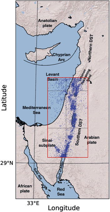
FIGURE 1. Tectonic setting for Israel and seismic map of the earthquakes included in the Israeli catalog. The red box is the area selected for the analysis.

Developing, implementing and delivering an OEF system for the State of Israel is indeed the final scope of the bilateral Italy-Israel project “Enhancing OPerational Earthquake foRecasting through innovative Approaches (OPERA)”, on request of the Israeli steering committee for earthquake preparedness, in collaboration with the Geophysical Institute of Israel. The scope is to provide the very first real-time operating tool, which brings the State of Israel into alignment with several other countries’ direction towards the release of reliable, live earthquake forecasts. Although the OEF system presented here is a prototype, it is an important first step which we trust can help the Israeli government agency and population to take pondered and calibrated actions aimed at reducing seismic hazard.

The first version of the OEF system presented here is based on the stochastic Epidemic Type Earthquake Sequence (ETES) model (Console and Murru, 2001; Giuseppe Falcone et al., 2010), which belongs to the general class of the self-exciting Epidemic Type Aftershock Sequence (ETAS) models firstly introduced by Ogata in 1988 (Ogata, 1988; Ogata, 1989; Ogata, 1998). The basic rational behind these models relies on the idea that seismic events cluster in space and time. In fact, this kind of spatiotemporal earthquake clustering models has been found to be the most reliable to track the probabilistic evolution of the seismic process (Marzocchi et al., 2017; Taroni et al., 2018). In this paper, we set up the ETES model specific for the Israeli seismicity, and we also check the consistency of the forecasts with the data contained in the Israeli seismic catalog (https://earthquake.co.il/en/earthquake/searchEQS.php) carrying out two statistical tests proposed by the Collaboratory for the Study of Earthquake Predictability (CSEP), which is an international organization aimed at evaluating quantitatively earthquake predictions and forecasts at a global scale (https://cseptesting.org/) (Schorlemmer et al., 2018).

The evaluation of the forecasts produced can help highlighting advantages and room for improvement of the OEF-Israel system, as well as giving possible hints to adjust the same experiment in other countries.

2 Israeli Tectonic Setting

The Dead Sea Transform (DST), known also as the Dead Sea Fault, is the largest fault system of the Eastern-Mediterranean area, place of the strongest earthquakes in the last centuries (Meghraoui et al., 2003). It has been formed during the Miocene due to the African-Arabian plate collision with the Gulf of Aden southward of the Red Sea, which caused the separation of the Sinai subplate. The Israeli region is located in the southern section of the DST fault system (see Figure 1), but it is affected also by the seismic activity occurring in the middle DST, that is a restraining bend characterized by transpression deformation (Quennell, 1959). The region consists of a topographic valley with raised flanks and normal fault boarders. Tectonic movements occur on oblique- and left strike-slip fault segments, delineating a string of rhomb-shaped, narrow and deep sectors releasing bends linked to orthogonal separation of the transform flanks on the surface, that could also extend well beneath the crust (Garfunkel and Ben-Avraham, 2001; Wetzler et al., 2014). This is the most active tectonic region in the Eastern-Mediterranean area, as witnessed by the several prehistorical, historical and more recent large earthquakes (Amit et al., 2002; Baer et al., 2008; Marco, 2008). A spatial distribution analysis of seismic events (Sharon et al., 2019) allowed to identify criteria for sorting the active faults in the region as “main strike-slip faults of the DST” and “faults with direct evidence of Quaternary activity,” which are shown in the map available at the following link (see also Fig7 of Sharon et al. (2019)). As shown in the next subsection, and by comparing Figure 1 and the map of the url above, the complete dataset considered in this paper involves the main strike-slip faults of the DST and surrounding areas, as well as marginal faults, main branches and quaternary activity. The segments involved are Dakar fault, passing through Arava and Eastern/Western Dead Sea faults, until the further north Jordan Gorge and Roums faults.

3 The First Operational Earthquake Forecasting System of Israel

3.1 The Philosophy of the OEF-Israel System

We adopt the same philosophy of the OEF-Italy system which is rooted in three main pillars. In particular, the OEF-Israel system 1) is fully transparent, such that the results are reproducible by anyone, expert or not in the field, who is interested in knowing and understanding the earthquake probabilistic forecast in the spatio-temporal window of interest; 2) is open to any modelers who want to contribute for future developments (the Italian system requires that any additional model has to be submitted to at least one CSEP experiment); 3) minimizes scientific controversies. To be more specific on this latter point, the idea is to use ensemble models built as the weighted combination of two or more models, where the weights are obtained from the objective statistical evaluation of each of the constitutive models’ performance, thus significantly reducing the implicit subjectivity induced by selecting a single model. An ensemble model is not yet implemented in this pilot OEF-Israel system because we consider here only one model, the ETES model; however, this functionality can be activated when additional models will be added.

3.2 ETES Model

The earthquake forecasting model adopted in the OEF system for Israel is the clustering, self-exciting Epidemic Type Earthquake Sequence (ETES) model proposed in Giuseppe Falcone et al. (2010) and previously introduced in Console and Murru (2001) and Console et al. (2007). According to this purely stochastic model, the conditional probability density function quantifying the occurrence rate of a seismic event (x, y, t, M) is given by

$\lambda (x,y,t,M|{\mathcal{H}}_t)=f_R\cdot {\lambda }_0(x,y,M)+\sum _{i=1}^{N}H(t-t_i){\lambda }_i(x,y,t,M),(1)$

where: ${\mathcal{H}}_t$ is the past history of the current event; f_R is the “failure rate” function, i.e., the ratio between the expected number of independent events and the total number of shocks; λ₀ (x, y, M) is the time-invariant “spontaneous” background seismicity, obtained by analyzing a real seismic catalog using a smoothing algorithm; H (⋅) is a step function and λ_i (x, y, t, M) is the punctual contribution of the past ith event (x_i, y_i, t_i, M_i). The summation performed over the contributions of all the previous shocks, that is the second term in the right hand side of the ETES rate (1), provides the time-varying “triggered” aftershock component of the seismic sequence. According to the ETES model, the magnitude distribution of both the spontaneous and triggered components of rate (1) is separable with respect to time and space, and it is given by the well-known decreasing exponential Gutenberg-Richter law (Gutenberg and Richter, 1944)

$p(M)=10^{-b(M-M_c)},M\ge M_c,(2)$

where M_c is the completeness magnitude, that is the value such that all the events with a higher magnitude are surely recorded in the earthquake catalog (Mignan and Woessner, 2012). The parameter b is the so-called b-value, which controls the slope of the magnitude-frequency distribution in a semi-log plot: the higher is this parameter, the lower is the fraction of larger shocks with respect to the smaller ones; some authors claim that a decrease of the b-value can be interpreted as a precursor for forthcoming large shocks, but this is actually an open debate in the literature due to the potential sources of bias that can affect this parameter’s estimation (Marzocchi et al., 2020). The time-independent background function λ₀ (x, y, M) is obtained through the method introduced by Frankel (1995), with an exponential kernel distribution adopted for the smoothing algorithm. The triggered component λ_i (x, y, t, M) of rate (1) is given by

${\lambda }_i(x,y,t,M)=\mathrm{\Phi }(t-t_i)\cdot \mathrm{\Psi }(r)\cdot p(M),(3)$

where $\mathrm{\Phi }(t-t_i)=\frac{k}{{(t-t_i+c)}^p}$ is the modified Omori law for the temporal decay, and

$\mathrm{\Psi }(r)={\left[\frac{d_i^2}{r^2+d_i^2}\right]}^q,d_i=d_0\cdot 10^{\alpha (M_i-M_c)},(4)$

is the isotropic spatial function of the distance r between the location of the current event (x, y) and the location of the previous event (x_i, y_i). Following Giuseppe Falcone et al. (2010), in the function d_i we set $\alpha =\frac{1}{2}$, so that the average triggering distance of the aftershock zone is proportional to the square root of the mainshock rupture area, as observed for real data (Kagan, 1991). We note that when α is not fixed a priori, but it is estimated, and when the spatial function is Gaussian, the model is switched to the classical ETAS (Ogata, 1998).

The ETES parameters (p, c, k, d₀, q, b) are assumed to be positive and typically estimated through the maximum likelihood function technique (Aki, 1965; Bender, 1983; Ogata, 1988; Ogata, 1998; Marzocchi and Sandri, 2003). These estimates are performed by considering a learning period of the seismic catalog, and they are then used in the model to forecast future earthquake events.

3.3 OEF System Interface

The forecasts are available to users of the system by means of a comprehensive and interactive dashboard composed of an embedded Google Maps showing 1) the current weekly probability map, 2) a timeline graph showing the probability history for a single cell or area, and 3) the current probability values for a selected cell or geographical area (Figure 2). All probability maps and the time evolution of the probability for each single cell are stored for future reference and quick access. In this way, users can query the database by name of location (inverse geocoding) or by direct selection of a point or area on the map, and plot the evolution of the probability in any time window of interest.

FIGURE 2

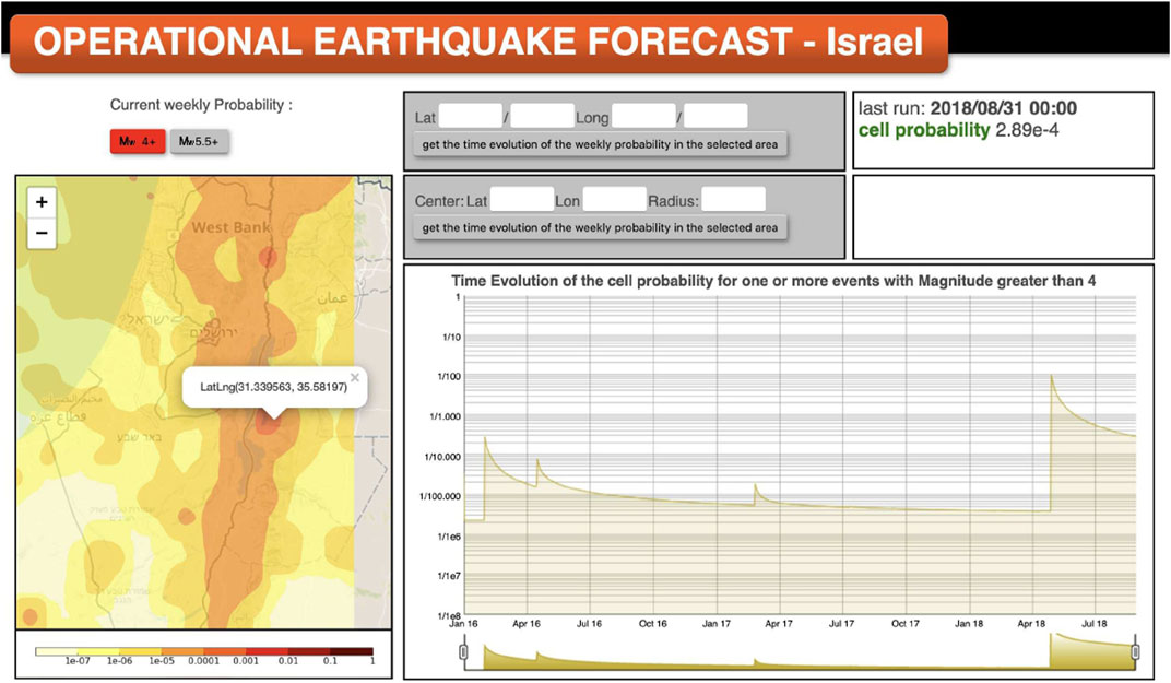
FIGURE 2. A snapshot of the OEF-Israel forecasting system. The interactive dashboard composed of (left) an embedded Google Maps showing the current weekly probability map for moment magnitude M_w ≥ 4 and M_w ≥ 5.5. On the lower right, a timeline graph shows the probability history for a cell marked on the map of Israel. The upper right part reports the probabilities of the last run of the system.

4 Preliminary OEF Application in Israel

4.1 Israeli Seismic Catalog

The instrumental earthquake data in the State of Israel have been collected since the beginning of the 20th century by seismic stations in Egypt, Lebanon, Israel [Geophysical Institute of Israel/GEOFOrschungsNetz Station Jerusalem (JER), GEOFOrschungsNetz Station Eilat (EIL)] and several tens of stations in Europe. More precisely, the complete earthquake catalog in the period 1900–1982 has been recorded by the International Seismological Summary (ISS), the International Seismological Centre (ISC), the National Earthquake Information Center (NEIC), and the compilation of Arieh et al. (1985). From 1982 on, seismic data have instead been recorded by the two national seismic networks of the State of Israel and Jordan. The first, named the Israel Seismic Network (ISN), was established in 1982 and is operated continuously by the Seismology Division of the Geophysical Institute of Israel (GII); the second, named the Jordanian Seismic Network (JSN), was established in 1983 and is operated continuously by the Jordan Seismo Obs and Geo Studies–Natural Resources Authority (NRA) of the Hashemite Kingdom of Jordan.

The complete dataset used for magnitude analysis counts 31,322 events in the time span from 1900 to 2020 covering a large area extending also beyond the Israeli boundaries, as shown in Figure 1. Since we focus on the area of the State of Israel, we restrict the analysis to the region included in the latitudes 29.4° N–34° N and longitudes 33.9° E–36.3° E (red box in Figure 1). The number of events in this smaller area is 10,340. We also integrated the catalog with 5 events with M_w in the range [4.8, 5.3] reported by the “Global Centroid Moment Tensor” (Global-CMT) database in the selected area. The analysis of the events’ magnitudes in the considered catalog has shown a lot of heterogeneity. Duration, body and moment magnitudes have been adopted singularly or jointly to describe the size of the events, depending on the geographical location or on the type of energy released. To eliminate this source of uncertainty that would invalidate the reliability of the forecasts, we have developed a new catalog where the magnitudes have been homogenized through the General Orthogonal Regression (GOR) technique (Lolli and Gasperini, 2012). For the details, see the Supplementary Appendix.

4.2 Learning Phase

We selected the period from January 1, 1983 to December 31, 2015 for the learning period, as it was found to reproduce the best fit of the model parameters. It contains 1,690 events within 30 km depth and of magnitude ≥2.2, the latter being the completeness threshold value computed through the maximum curvature method (Wiemer and Wyss, 2000). The correlation distance of 9 km was adopted in the exponential kernel distribution of the smoothing algorithm, as determined by maximizing the log-likelihood function of the seismicity contained in half of the catalog, under the time-independent model obtained from the other half. We recall that the log-likelihood function of the ETES model in the spatiotemporal domain [0, T] × S is given by

$\mathrm{l}\mathrm{o}\mathrm{g}L(\theta )=\sum _{i=1}^N\mathrm{l}\mathrm{o}\mathrm{g}{\lambda }_{\theta }(x,y,t,M|{\mathcal{H}}_t)-{\int }_0^T{\iint }_S{\lambda }_{\theta }(x,y,t,M|{\mathcal{H}}_t)dxdydt,$

where θ is the set of parameters. Since a future earthquake could occur also in an area of low or null observed seismicity, we labeled the cells of a square lattice covering the whole region with the 1% of the total rate, divided by the total number of cells (surprise coefficient), as in Kagan and Jackson (2000). The seismicity rate of the learning catalog is shown in Figure 3, together with the estimates for the model parameters (p, c, k, d₀, q). Since some physical investigations show that the static stress changes decrease with epicentral distance as r⁻³ (Hill et al., 1993; Antonioli et al., 2004), for the sake of simplicity and following the line of several papers in the literature (Lombardi and Marzocchi, 2010b; Giuseppe Falcone et al., 2010) here we impose that q = 1.5. This is a value close to that obtainable from the maximum likelihood best fit, and which follows the theory of elasticity when the spatial distance from the triggering event tends to infinite; the recognized trade-off between q and the other spatial parameter d₀ also justifies this choice, in fact different pairs (q, d₀) are shown to provide almost the same model’s likelihood (Kagan and Jackson, 2000).

FIGURE 3

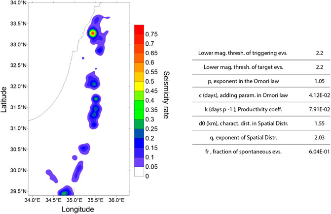
FIGURE 3. Smoothed seismicity of the Israeli seismic catalog in the learning period January 01, 1983–December 31, 2015. The correlation distance is 9 km. The color scale represents the number of earthquakes with M ≥ 2.2 and depth ≤30 km, in a 1 km² area, over the whole time period spanned by the catalog. The list of the model parameters and their corresponding values are shown on the right.

4.3 Forecasting Phase

The forecasting test we carried out in the OEF experiment for Israel has been implemented from January 01, 2016 till November 15, 2020, in the spatial extent [29.4°N, 34°N] latitude × [33.9°E, 36.3°E] longitude, gridded in a 0.1 ° × 0.1 ° square lattice covering the entire region.

As preliminary OEF experiment presented here, for the sake of simplicity we use in the whole forecasting period the same parameters set estimated in the learning phase. This is also justified by the fact that the ETES model has been shown to be able to track the seismic variability even with constant parameters, as shown for example in the case of Tohoku M_w nine earthquake, when ETES performed better than models with varying parameters (Nanjo et al., 2012). In any case, our future scope (and work in progress) is to improve the reliability of the forecast by following the Bayesian approach, which consists in daily or weekly updating the parameter estimations (Omi et al., 2013; Omi et al., 2015).

In this OEF experiment, each day of the temporal window specified above we produce weekly forecasts of the expected rates (or probabilities) of earthquakes with magnitudes $\ge {\bar{M}}_w$, where ${\bar{M}}_w=4.0$ and 5.5. These two threshold can be re-set in the future for any magnitude or macroseismic intensity threshold, that are of interest for the stakeholders. We also stress that the choice of 7-days forecasts has been inherited from OEF-Italy, as an explicit request from Italian Civil Protection to have short-term forecasts within a temporal window reasonable to activate state of alert procedures; anyway, the forecasts are produced at the midnight of ever day, and after the occurence of any M_w ≥ 3.5 event recorded by the seismic network, therefore the government agency can modify the forecating time window according their specifici needs.

The output produced by the system is the same as illustrated for Italy in Marzocchi et al. (2014): time-dependent maps showing the weekly probability for $M_w\ge {\bar{M}}_w$ earthquakes occurring in each cell of the spatial grid covering the analyzed region. As an example, we show in Figure 4 the forecast of M_w ≥ 4.0 events produced for the week starting from August 31, 2018, 00:00 UTC; see also Figure 2. The map shows that on August 31 the OEF forecast have conferred a maximum of probability in the cells of the grid covering the Sea of Galilee, on the city of Tiberias, each cell having a probability of about 10⁻³ for M_w ≥ 4.0 earthquakes. This maximum is caused by the occurrence, 1 month before, by a M_w 4.7 event which induced an increase of the moderate earthquake rate. Besides this maximum in probability, the map shows also a peristent higher probability along the Death Sea valley as expected by the higher rate of historical seismicity.

FIGURE 4

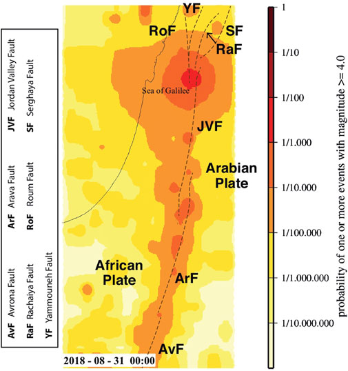
FIGURE 4. Probability map (gridded on a lattice of 0.1 ° × 0.1 ° cells) of one or more events with M_w ≥ 4.0 to occur in the week starting from August 31, 2018 at 00:00 UTC. The dashed lines indicate the faults involved in the analyzed area and the names of the plates are also included; see also Figure 2.

4.4 Testing Phase

In this section we discuss in detail the testing analysis of the produced forecasts’ reliability.

The testing phase of the model is carried out following the guidelines of the Collaboratory for the Studies of Earthquake Predictability (CSEP). Specifically, the N-test and S-test are performed to assess the reliability of the delivered forecast for Israel, i.e., to test the consistency of the OEF forecasts with the earthquakes occurred.

The N-test evaluates the consistency between the number N_fore of forecasted earthquakes in all space-time-magnitude bins, and the number N_obs of events observed over the entire testing region within any forecasting time window, and over any magnitude larger than the selected threshold. The two-tailed p-value is obtained by assuming that the target earthquakes follow the Poisson distribution with N_fore mean. More precisely, given the collection J of synthetic catalogs representing the forecast, and the relative empirical cumulative distribution functions ${\{F_{N_{fore,j}}\}}_{j\in J}$, the test is performed by computing the two quantile scores

$\begin{array}{ll}\hfill {\delta }_1& =1-F_{N_{fore,j}}\left(N_{obs}-1\right)=\mathbb{P}(N_{fore,j}\ge N_{obs}),\hfill \\ \hfill {\delta }_2& =F_{N_{fore,j}}\left(N_{obs}\right)=\mathbb{P}(N_{fore,j}\le N_{obs})\hfill \end{array}$

The result of the test indicates an over–predicting or under–predicting forecast, respectively, when δ₁ or δ₂ goes below a critical threshold value, which in our case corresponds to the 0.01 significant level (Taroni et al., 2018).

The S-test evaluates consistency of spatial occurrence of target events with respect to the model’s normalized spatial forecast. The spatial component of the forecast is isolated, and the forecast is normalized so that its sum matches the observation. The test is then summarized by the quantile score

$\zeta =\frac{\#\left\{S_X|S_X\le S,S_X\in S_S\right\}}{\#\left\{S_S\right\}},$

that is the fraction of simulated synthetic catalogs of target earthquakes having spatial log likelihoods $\left\{S_X\right\}$ smaller than the observed spatial log likelihood S, calculated with the observed target earthquakes ($\left\{S_S\right\}$ is the set of all the simulated spatial likelihoods). This quantile score represents also the p-value of the S-test. An inconsistent forecast is then obtained from the latter when ζ falls below the significance level fixed for this test, which we set here at 0.01. More precisely, a small p-value indicates that the fit between forecasts and data is worse than the one expected if the model was generating the data (Taroni et al., 2018). We stress that we use the 1% significance level since the N- and S-tests are susceptible to the use of a Poisson assumption; in fact, target earthquakes are expected to follow overdispersed distributions but, from its perspective, the Poisson assumption could induce the rejection of models that capture such overdispersion (Lombardi and Marzocchi, 2010a), like it happens for the ETES model adopted in the OEF-system for Israel.

We apply the N- and S-tests for all the 255 weekly windows entirely included in the forecasting phase, that is, 255 weeks starting from the first Sunday after January 1, 2016, occurred on January 3. The target events are those with magnitude M_w ≥ 3: we use the rescaling technique to obtain the relative probabilities from the forecasts produced for the events ≥4.0. In the 255 weekly testing windows we found 48 target events, distributed as in Figure 5A. The consistency of the ETES model is found positive for N- and the p-value obtained is shown in Figure 5B. The S-Test results are presented in Figure 5C, and indicate that the cumulative p-value trend is not always positive and that in some cases it falls below the significance level 0.01. This could be due to the occurrence of small earthquakes with M_w = 3 in regions with expected low seismicity rate. In any case, we also calculate the S-test by considering as target the few events with M_w ≥ 4, that is the same threshold adopted in the learning period. In this case, the resulting p-values fall completely above the significance level 0.01 for the pair of events occurring within the 255th week (Figure 5D). The corresponding N-test is shown in Figure 5E.

FIGURE 5

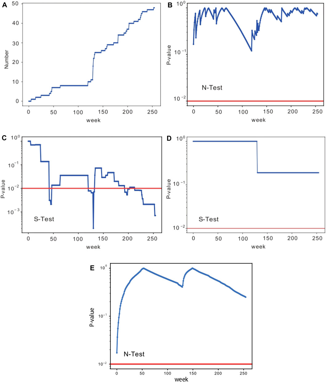
FIGURE 5. (A): cumulative number of M_w ≥ 3 events in the Israeli catalog versus time. (B) and (C): p-values versus time of the N- and the S-tests, respectively, obtained for the ETES model. The horizontal red lines indicate the 0.01 significance level. In all the plots, the x-axis represents the weeks starting from January 3, 2016. (D) and (E): p-value of respectively the S- and N-test obtained for the ETES model with M_w ≥ 4.

5 Discussion and Conclusion

Since deterministic earthquake prediction is still an elusive enterprise, growing efforts are dedicated to deliver reliable earthquake forecasts which may help communities to be prepared and possibly to reduce the number of casualties. In line with this goal, in this paper we presented the development of the first Operational Earthquake Forecasting system for the State of Israel. In fact, the governmental Israeli steering committee for earthquake preparedness expressed interest in developing and implementing a real-time OEF system to reduce seismic hazard in Israel, on the basis of the prototipe developed for Italy. This resulted in the bilater Italy-Israel OPERA project, to whose final scope this paper responds.

This pilot OEF-Israel system is based on the stochastic clustering ETES model, and it is implemented similar to the Italian system (Marzocchi et al., 2014). We have considered the time window 1900–2020 and the spatial extent [29.4°N, 34°N] latitude × [33.9°E, 36.3°E] longitude, which covers the land of Israel.

The set of the model parameters and the background seismicity have been estimated through a maximum likelihood approach using a learning period of about 32 years. Then we have produced earthquake forecasts for Israel. In each day between January 3, 2016 and November 15, 2020 we have delivered weekly forecasts for M_w ≥ 4.0 and M_w ≥ 5 events in the area [29.4°N, 34°N] latitude × [33.9°E, 36.3°E] longitude, providing time-dependent seismic maps of the relative expected rates. An example is illustrated in Figure 4 for the M_w ≥ 4.0 events produced in the week starting from August 31, 2018, 00:00 UTC. This map shows an increase in probability around the Sea of Galilee that was caused by the M_w 4.7 event which occurred in this region a few days before.

The reliability of the OEF forecasts have been checked by adopting the CSEP guidelines. In particular, we have performed the N-test and the S-test to analyze the outcomes relative to M_w ≥ 3 target events occurred during the 255 weeks entirely contained in the forecasting temporal window. We have obtained satisfactory results for both tests, with only a 2% overestimation of the predicted events with respect to the observed ones. The spatial distribution is also well captured by the model most of the time. However, we have found a few cases in which the p-value is particularly low for the S-test; this is due to the occurrence of a moderate seismicity in the testing area in areas where a low activity is expected. This calls for the need of considering improved alternative models (stand-alone and/or in an ensemble approach), for the aim of obtaining more reliable spatial distributions. Some new models have already been proposed in the literature by some Israeli colleagues (Zhang et al., 2021), and this will be the object of future further studies. As a preliminary experiment, we are confident that the OEF system we developed in this paper for the State of Israel could be an additional tile that, reinforced in its weaknesses, will allow pursuing the aim of delivering real-time probabilistic forecasts worldwide.

Data Availability Statement

The datasets used for this study can be found at the links: https://earthquake.usgs.gov/data/iss_summ.php (ISS), http://www.isc.ac.uk (ISC), https://earthquake.usgs.gov/contactus/golden/neic.php, https://www.fdsn.org/networks/detail/IS/ (ISN), https://www.gii.co.il (GII), https://www.fdsn.org/networks/detail/JS/ (JSN), https://www.globalcmt.org (Global-CMT).

Author Contributions

All authors contributed to the conception and design of the study, which has been developed in the framework of the Italy-Israel bilateral project OPERA coordinated by SH and WM. GF organized the database and implemented the software codes; GF, IS, and WM performed the statistical analysis. GF and IS wrote most of the paper with contributions from all the other authors. All authors reviewed and approved the submitted version.

Funding

This work has been supported by the bilateral Italy-Israel project “Enhancing OPerational Earthquake foRecasting through innovative Approaches (OPERA)”, which has been funded by the Ministry of foreign affairs and international cooperation of the Italian republic and the Ministry of science, technology and space of the State of Israel, and by the Real-time Earthquake Risk Reduction for a Resilient Europe (RISE) project, funded by the European Unions Horizon 2020 research and innovation program (Grant Agreement Number 821115).

Conflict of Interest

The authors declare that the research was conducted in the absence of any commercial or financial relationships that could be construed as a potential conflict of interest.

Publisher’s Note

All claims expressed in this article are solely those of the authors and do not necessarily represent those of their affiliated organizations, or those of the publisher, the editors and the reviewers. Any product that may be evaluated in this article, or claim that may be made by its manufacturer, is not guaranteed or endorsed by the publisher.

Acknowledgments

The authors thank Matteo Taroni for helpful discussions on the testing phase of the model.

Supplementary Material

The Supplementary Material for this article can be found online at: https://www.frontiersin.org/articles/10.3389/feart.2021.729282/full#supplementary-material

References

Aki, K. (1965). Maximum Likelihood Estimate of B in the Formula Log N = a - Bm and its Confidence Limits. Bull. Earthq. Res. Inst. Tokyo Univ. 43, 237–239.

Google Scholar

Amit, R., Zilberman, E., Enzel, Y., and Porat, N. (2002). Paleoseismic Evidence for Time Dependency of Seismic Response on a Fault System in the Southern Arava Valley, Dead Sea Rift, Israel. GSA Bull. 114, 192–206. doi:10.1130/0016-7606(2002)114<0192:peftdo>2.0.co;2

CrossRef Full Text | Google Scholar

Antonioli, A., Belardinelli, M. E., and Cocco, M. (2004). Modelling Dynamic Stress Changes Caused by an Extended Rupture in an Elastic Stratified Half-Space. Geophys. J. Int. 157, 229–244. doi:10.1111/j.1365-246X.2004.02170.x

CrossRef Full Text | Google Scholar

Arieh, E., Artzi, D., Benedik, N., Eckstein, A., Issakow, R., Reich, B., et al. (1985). Revised and Updated Catalog of Earthquakes in Israel and Adjacent Areas, 1900–1980. Inst. Petrol. Res. Geophys. Z6/121683, 8699–8711.

Google Scholar

Baer, G., Funning, G. J., Shamir, G., and Wright, T. J. (2008). The 1995 November 22,Mw7.2 Gulf of Elat Earthquake Cycle Revisited. Geophys. J. Int. 175, 1040–1054. doi:10.1111/j.1365-246x.2008.03901.x

CrossRef Full Text | Google Scholar

Bender, B. (1983). Maximum Likelihood Estimation of B Values for Magnitude Grouped Data. Bull. Seismol. Soc. Am. 73, 831–851. doi:10.1785/bssa0730030831

CrossRef Full Text | Google Scholar

Console, R., and Murru, M. (2001). A Simple and Testable Model for Earthquake Clustering. J. Geophys. Res. 106, 8699–8711. doi:10.1029/2000JB900269

CrossRef Full Text | Google Scholar

Console, R., Murru, M., Catalli, F., and Falcone, G. (2007). Real Time Forecasts Through an Earthquake Clustering Model Constrained by the Rate-And-State Constitutive Law: Comparison With a Purely Stochastic ETAS Model. Seismological Res. Lett. 78, 49–56. doi:10.1785/gssrl.78.1.49

CrossRef Full Text | Google Scholar

Frankel, A. (1995). Mapping Seismic Hazard in the Central and Eastern United States. Seismological Res. Lett. 66, 8–21. doi:10.1785/gssrl.66.4.8

CrossRef Full Text | Google Scholar

Garfunkel, Z., and Ben-Avraham, Z. (2001). Basins along the Dead Sea Transform. Mémoires du Muséum Natl. d’histoire naturelle (1993). 186, 607–627.

Google Scholar

Gerstenberger, M., Mcverry, G., Rhoades, D., and Stirling, M. (2014). Seismic Hazard Modeling for the Recovery of Christchurch. Earthquake Spectra. 30, 17–29. doi:10.1193/021913EQS037M

CrossRef Full Text | Google Scholar

Giuseppe Falcone, G., Rodolfo Console, R., and Maura Murru, M. (2010). Short-Term and Long-Term Earthquake Occurrence Models for Italy: ETES, ERS and LTST. Ann. Geophys. 53, 41–50. doi:10.4401/ag-4760

CrossRef Full Text | Google Scholar

Gutenberg, B., and Richter, C. F. (1944). Frequency of Earthquakes in California. Bull. Seismol. Soc. Am. 34, 185–188. doi:10.1785/bssa0340040185

CrossRef Full Text | Google Scholar

Hill, D. P., Reasenberg, P. A., Michael, A., Arabaz, W. J., Beroza, G., Brumbaugh, D., et al. (1993). Seismicity Remotely Triggered by the Magnitude 7.3 Landers, California, Earthquake. Science. 260, 1617–1623. doi:10.1126/science.260.5114.1617

PubMed Abstract | CrossRef Full Text | Google Scholar

[Dataset] Hofstetter, A., and Ataev, G. (2012). The Use of P-Wave Spectra in the Determination of Earthquake Source Parameters in IsraelReport No: 569/701/12. https://earthquake.co.il/docs/Reports/2012_569-701-12.pdf

Google Scholar

Jordan, T. H., Marzocchi, W., Michael, A. J., and Gerstenberger, M. C. (2014). Operational Earthquake Forecasting Can Enhance Earthquake Preparedness. Seismological Res. Lett. 85, 955–959. doi:10.1785/0220140143

CrossRef Full Text | Google Scholar

Kagan, Y. Y., and Jackson, D. D. (2000). Probabilistic Forecasting of Earthquakes. Geophys. J. Int. 143, 438–453. doi:10.1046/j.1365-246X.2000.01267.x

CrossRef Full Text | Google Scholar

Kagan, Y. Y. (1991). Likelihood Analysis of Earthquake Catalogues. Geophys. J. Int. 106, 135–148. doi:10.1111/j.1365-246X.1991.tb04607.x

CrossRef Full Text | Google Scholar

Kurzon, I., Nof, R. N., Laporte, M., Lutzky, H., Polozov, A., Zakosky, D., et al. (2020). The "TRUAA" Seismic Network: Upgrading the Israel Seismic Network-Toward National Earthquake Early Warning System. Seismological Res. Lett. 91, 3236–3255. doi:10.1785/0220200169

CrossRef Full Text | Google Scholar

Lilliefors, H. W. (1969). On the Kolmogorov-Smirnov Test for the Exponential Distribution with Mean Unknown. J. Am. Stat. Assoc. 64, 387–389. doi:10.1080/01621459.1969.10500983

CrossRef Full Text | Google Scholar

Lolli, B., and Gasperini, P. (2012). A Comparison Among General Orthogonal Regression Methods Applied to Earthquake Magnitude Conversions. Geophys. J. Int. 190, 1135–1151. doi:10.1111/j.1365-246X.2012.05530.x

CrossRef Full Text | Google Scholar

Lombardi, A. M., and Marzocchi, W. (2010a). The Assumption of Poisson Seismic-Rate Variability in CSEP/RELM Experiments. Bull. Seismological Soc. America. 100, 2293–2300. doi:10.1785/0120100012

CrossRef Full Text | Google Scholar

Lombardi, A. M., and Marzocchi, W. (2010b). The ETAS Model for Daily Forecasting of Italian Seismicity in the CSEP experiment. Ann. Geophys. 53, 2293–2300. doi:10.4401/ag-4848

CrossRef Full Text | Google Scholar

Marco, S. (2008). Recognition of Earthquake-Related Damage in Archaeological Sites: Examples From the Dead Sea Fault Zone. Tectonophysics. 453, 148–156. doi:10.1016/j.tecto.2007.04.011

CrossRef Full Text | Google Scholar

Marzocchi, W., Lombardi, A. M., and Casarotti, E. (2014). The Establishment of an Operational Earthquake Forecasting System in Italy. Seismological Res. Lett. 85, 961–969. doi:10.1785/0220130219

CrossRef Full Text | Google Scholar

Marzocchi, W., Taroni, M., and Falcone, G. (2017). Earthquake Forecasting During the Complex Amatrice-Norcia Seismic Sequence. Sci. Adv. 3, e1701239. doi:10.1126/sciadv.1701239

PubMed Abstract | CrossRef Full Text | Google Scholar

Marzocchi, W., Spassiani, I., Stallone, A., and Taroni, M. (2020). Erratum to: How to Be Fooled Searching for Significant Variations of the B-Value. Geophys. J. Int. 221, 351. doi:10.1093/gji/ggaa061

CrossRef Full Text | Google Scholar

Marzocchi, M., and Sandri, L. (2003). A Review and New Insights on the Estimation of the B-Valueand its Uncertainty. Ann. Geophys. 46. doi:10.4401/ag-3472

CrossRef Full Text | Google Scholar

Meghraoui, M., Gomez, F., Sbeinati, R., Van der Woerd, J., Mouty, M., Darkal, A. N., et al. (2003). Evidence for 830 Years of Seismic Quiescence From Palaeoseismology, Archaeoseismology and Historical Seismicity along the Dead Sea Fault in Syria. Earth Planet. Sci. Lett. 210, 35–52. doi:10.1016/s0012-821x(03)00144-4

CrossRef Full Text | Google Scholar

Michael, A. J., McBride, S. K., Hardebeck, J. L., Barall, M., Martinez, E., Page, M. T., et al. (2020). Statistical Seismology and Communication of the USGS Operational Aftershock Forecasts for the 30 November 2018 Mw 7.1 Anchorage, Alaska, Earthquake. Seismological Res. Lett. 91, 153–173. doi:10.1785/0220190196

CrossRef Full Text | Google Scholar

Mignan, A., and Woessner, J. (2012). Estimating the Magnitude of Completeness for Earthquake Catalogs. Community Online Resource Stat. Seismicity Anal., 1–45. doi:10.5078/corssa-00180805

CrossRef Full Text | Google Scholar

Nanjo, K. Z., Tsuruoka, H., Yokoi, S., Ogata, Y., Falcone, G., Hirata, N., et al. (2012). Predictability Study on the Aftershock Sequence Following the 2011 Tohoku-Oki, Japan, Earthquake: First Results. Geophys. J. Int. 191, 653–658. doi:10.1111/j.1365-246X.2012.05626.x

CrossRef Full Text | Google Scholar

Ogata, Y. (1988). Statistical Models for Earthquake Occurrences and Residual Analysis for Point Processes. J. Am. Stat. Assoc. 83, 9–27. doi:10.1080/01621459.1988.10478560

CrossRef Full Text | Google Scholar

Ogata, Y. (1989). Statistical Model for Standard Seismicity and Detection of Anomalies by Residual Analysis. Tectonophysics. 169, 159–174. doi:10.1016/0040-1951(89)90191-1

CrossRef Full Text | Google Scholar

Ogata, Y. (1998). Space-Time Point-Process Models for Earthquake Occurrences. Ann. Inst. Stat. Mathematics. 50, 379–402. doi:10.1023/a:1003403601725

CrossRef Full Text | Google Scholar

Omi, T., Ogata, Y., Hirata, Y., and Aihara, K. (2013). Forecasting Large Aftershocks Within One Day after the Main Shock. Sci. Rep. 3, 2218. doi:10.1038/srep02218

PubMed Abstract | CrossRef Full Text | Google Scholar

Omi, T., Ogata, Y., Hirata, Y., and Aihara, K. (2015). Intermediate-Term Forecasting of Aftershocks From an Early Aftershock Sequence: Bayesian and Ensemble Forecasting Approaches. J. Geophys. Res. Solid Earth. 120, 2561–2578. doi:10.1002/2014JB011456

CrossRef Full Text | Google Scholar

Quennell, A. M. (1959). Tectonics of the Dead Sea Rift. Proc. 20th Int. Geol. congress, Mexico. 385, 403.

Google Scholar

Schardong, L., Horin, Y. B., Ziv, A., Myers, S. C., Wust-Bloch, H., and Radzyner, Y. (2021). High-Quality Revision of the Israeli Seismic Bulletin. Seismological Res. Lett. 92, 2668–2678. doi:10.1785/0220200422

CrossRef Full Text | Google Scholar

Schorlemmer, D., Werner, M. J., Marzocchi, W., Jordan, T. H., Ogata, Y., Jackson, D. D., et al. (2018). The Collaboratory for the Study of Earthquake Predictability: Achievements and Priorities. Seismol. Res. Lett. 89, 1305–1313. doi:10.1785/0220180053

CrossRef Full Text | Google Scholar

Shapira, A. (1988). Magnitude Scales for Regional Earthquakes Monitored in Israel. Isr. J. Earth-Sciences. 37, 17–22.

Google Scholar

Sharon, M., Sagy, A., Kurzon, I., Marco, S., and Rosensaft, M. (2020). Assessment of seismic sources and capable faults through hierarchic tectonic criteria: implications for seismic hazard in the Levant. Nat. Hazards Earth Syst. Sci., 20, 125–148. doi:10.5194/nhess-20-125-2020

CrossRef Full Text | Google Scholar

Taroni, M., Marzocchi, W., Schorlemmer, D., Werner, M. J., Wiemer, S., Zechar, J. D., et al. (2018). Prospective CSEP Evaluation of 1‐Day, 3‐Month, and 5‐Yr Earthquake Forecasts for Italy. Seismol. Res. Lett. 89, 1251–1261. doi:10.1785/0220180031

CrossRef Full Text | Google Scholar

Thomas, H. T., Yun-Tai Chen, Y., Paolo Gasparini, P., Raul Madariaga, R., Ian Main, I., Warner Marzocchi, M., et al. (2011). Operational Earthquake Forecasting. State of Knowledge and Guidelines for Utilization. Ann. Geophys., 173, 316–391. doi:10.4401/ag-5350

CrossRef Full Text | Google Scholar

Wetzler, N., Sagy, A., and Marco, S. (2014). The Association of Micro-Earthquake Clusters With Mapped Faults in the Dead Sea Basin. J. Geophys. Res. Solid Earth. 119, 8312–8330. doi:10.1002/2013jb010877

CrossRef Full Text | Google Scholar

Wiemer, S., and Wyss, M. (2000). Minimum Magnitude of Completeness in Earthquake Catalogs: Examples from Alaska, the Western United States, and Japan. Bull. Seismological Soc. America. 90, 859–869. doi:10.1785/0119990114

CrossRef Full Text | Google Scholar

Zhang, Y., Zhou, D., Fan, J., Marzocchi, W., Ashkenazy, Y., and Havlin, S. (2021). Improved Earthquake Aftershocks Forecasting Model Based on Long-Term Memory. New J. Phys. 23, 042001. doi:10.1088/1367-2630/abeb46

CrossRef Full Text | Google Scholar