An efficient local imaging strategy based on illumination analysis with deep learning

1 INTRODUCTION

Seismic imaging is to return the reflected wave or the diffracted wave to the underground location where it is generated. It mainly includes two parts: determining the spatial position of the reflection or diffraction point, and reproducing its waveform and amplitude characteristics. As the main step of seismic imaging, seismic migration is the process of moving the data signal from the receiver point to the underground position. In the 1960s, without considering the waveform characteristics of the reflected wave, seismic migration relied on manual operation to draw the spatial position of the reflection point. Claerbout (1971) proposed the wave equation migration technique. They used the finite difference method to solve the one-way wave equation, and reconstructed the wavefield propagating in the subsurface through observed data recorded by the geophone on the surface. The wavefield was extracted from the subsurface reflection interfaces to construct the migration profile. In the late 1970s, Stolt (1978) solved the wave equation in the frequency-wavenumber domain and extrapolated the seismic wavefield. The algorithm was called F-K domain migration. It had the characteristics of simple calculation and high efficiency, and had been quickly promoted in industry. The reverse time migration method was developed by solving the full wave equation for wavefield propagation (Baysal et al., 1983; McMechan, 1983). Chang et al. (1990) extended the reverse time migration method to the three-dimensional situation, and came up with the challenge of improving the accuracy and efficiency for 3D problems. Moreover, Wu et al. (1996) used high-order finite difference operators to achieve reverse time migration in three dimensions, and compared the features of high-order and low-order schemes. To compensate for poorly imaged areas, Chen and Jia (2014) proposed a staining algorithm for seismic modeling and imaging. This method performs dye marking on the target area and defines the staining wavefield. By imaging the target area with the staining wavefield, more accurate geology structures in the target area can be obtained. The staining algorithm based on reverse time migration establishes the connection between the real geological structure and its related wavefield and reflection data. Apart from reverse time migration, ray-based migration (Gray, 1986; Hill, 1990; Albertin et al., 2002) and one-way wave-equation-based migration (Ristow and Ruhl, 1994; Mulder and Plessix, 2004) are also commonly used in current practice.

Because of limited acquisition apertures, complex overburden structures, and large dipping angles, seismic migration often generates a distorted image of actual subsurface structures. (Lecomte, 1998) proposed the method of calculating the number of ground scattered wave coverage using ray tracing. The ray tracing-based illumination analysis provided directional illumination information, and the calculation speed was fast. The method only allowed for the seismic wave kinematic characteristics, and the calculation results are reliable when the medium is not seriously heterogeneous. In order to avoid the shortcomings of the ray-tracing based algorithm, wave theory is introduced into illumination analysis and has been successively applied to study illumination conditions under complex geology (Wu et al, 1996; Xie et al., 2003; Chen et al., 2007). Furthermore, Yang et al. (2008) put forward the idea of optimizing the design and acquisition system parameters by means of illumination analysis. Seismic illumination analysis can optimize the observation system so that the energy in the subsurface medium is evenly distributed (Xie et al., 2013). Moreover, Sun et al. (2018) proposed the multiple-wave-based illumination analysis method which is more powerful in evaluating and optimizing the observation system when dealing with complex geological models, and can make preliminary predictions on the imaging quality.

Machine learning (ML) offers algorithms designed to learn the features and relationships hidden in large datasets (Jia and Ma, 2017). As a branch of ML, deep learning has been widely applied to seismic model building, e.g., a prior models building from seismic images for full waveform inversion (Vigh et al., 2016), building detection framework based on deep learning model (Liu et al., 2018) and seismic tomography directly from shot gathers (Mauricio et al., 2018). In this paper, we first use deep learning method to establish the nonlinear relationship between the model and the illuminations, after training, it can help us got single-shot illumination result when inputting background velocity with shot information. Then, illumination results obtained by the network prediction can help us select the target area in which low illumination occurs densely. We further determine the low illumination area in target area of ​​the geological model and select partial shot sets to achieve high-resolution and high-efficiency imaging in low illumination areas.

2 ALGORITHM

2.1 Illumination theory

The two-dimensional constant density time domain acoustic wave equation has the form of:

$\frac{1}{v{\left(x,z\right)}^2}\frac{{\partial }^{2}u\left(x,z,t\right)}{\partial t^2}-{\mathrm{\nabla }}^{2}u\left(x,z,t\right)=s\left(t\right)(2.1)$

where $v\left(x,z\right)$ is the seismic wave velocity, $u\left(x,z,t\right)$ refers to the wavefield, and s(t) is the source.

The illumination intensity at point $\left(x,z\right)$ for a shot is defined as (Chen et al.,2013):

$I_s^{\left(i\right)}\left(x,z\right)={\displaystyle \sum _t{u}^{\left(i\right)}}\left(x,z,t\right).u^{\left(i\right)}\left(x,z,t\right),(2.2)$

where$I_s^{\left(i\right)}$ is the source illumination intensity for the i-th shot.

The source illuminance for N shots can be regarded as the sum of the illuminance for singleshot:

$\begin{array}{c}{I}_s\left(x,z\right) = {\displaystyle \sum }_{i=1}^N{I}_s^{\left(i\right)}\left(x,z\right).\end{array}(2.3)$

By obtaining the one-way (i.e., source-way) illumination intensity of single shot or multiple shots, we can investigate the distribution characteristics of the seismic wave energy propagating in the subsurface region. It provides a reference for redesigning the excitation position of the shot and the receiving range of the geophone. Although the distribution of subsurface energy can be seen through the one-way illumination diagram, it only indicates that the source energy can reach the specified subsurface location. Since not all these energy can be received by the surface geophone, it is necessary to consider factors such as the correspondence between excitation and detection, and the distribution of geophones on the surface.

As mentioned above, for a specified subsurface scattering point $\left(x,z\right)$, the energy intensity of the i-th shot is$I_s\left(x,z\right)$. We assume the energy received by the surface geophone for this point is$I_r^{\text{'}}\left(x_r,0\right)$where $x_r$ is the receiver location. According to the principle of wave reciprocity, the energy of the scattering point to the detection point can be converted into the energy $I_r\left(\text{x},z\right)$ received at $\left(x,z\right)$ with the excitation point of $\left(x_r,0\right)$.

We define the two-way illumination intensity of each source for a space point $\left(x,z\right)$as:

$\begin{array}{c}{I}_i\left(x,z\right)=\sqrt{I_s^{\left(i\right)}\left(x,z\right)I_r^{\left(i\right)}\left(x,z\right)}.\end{array}(2.4)$

The shots are independent of one another, and the same for geophones. Therefore, the two-way illumination intensity of M pairs of source and receiver can be regarded as the sum of each source-receiver pair, namely

$\begin{array}{c}I\left(x,z\right) = {\displaystyle \sum }_{i=1}^M{I}_i\left(x,z\right).\end{array}(2.5)$

2.2 Illumination analysis based on deep learning

For demonstration of combining deep learning and illumination analysis, we employ a simple method (Equations 2.2-2.5) to calculate the illumination, which costs little extra computational time in migration. When the geological model is large and complicated, it is necessary to adopt high-resolution illumination analysis methods, e.g., the local directional approaches (Mao et al., 2010; Yan & Xie, 2016), which require a lot of calculation time. The deep learning method can build the nonlinear mapping between the model and its corresponding single shot illumination result, and therefore efficient illumination analysis can be realized.

2.2.1 Building dataset

Since our illumination analysis is for geological models, we need to build a series of velocity models. In order to make the model represent as many complex subsurface features as possible, we randomly include flat layers, inclined formations, folds, faults, and high-velocity anomalies in the model. Figure 1 shows an example model generated by this means.

FIGURE 1

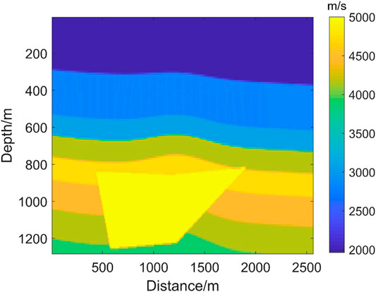
FIGURE 1. Randomly generated velocity model.

The desired output of the neural network is the single-shot source illuminance. The position information of the shot is crucial to the source illuminance. In order to include the shot information in the input of the network, we add a Gaussian function of point source at the shot position. For the shot position $\left(x_0, y_0\right)$, a two-dimensional Gaussian function is defined by

$f\left(x,y\right)=255\ast e^{-\left(\frac{{\left(x-x_0\right)}^2}{2c_{1}2}+\frac{{\left(y-y_0\right)}^2}{2c_2^2}\right)},(2.6)$

$\text{where}$$c_1$and $c_2$ are two variables in the x and y directions empirically determined by the radius of source illuminance.

In this way, we have the input of the neural network and calculate its corresponding output, with an example shown in Figure 2. From Figure 2A we see that the point source Gaussian function simulates the propagation mode of the seismic source very well. In the single-shot illumination result shown in Figure 2B, the energy near the sharp edge and below the high-velocity body is relatively weak. In this research, we built a total of 1,000 velocity models and got 25,000 single shot illumination results; therefore, the number of the training dataset including input and output is 25,000*2. The data set needs to be normalized before being applied to the network model. After data normalization, the process of searching for the best parameters of the network model will become smoother, and the normalization effectively prevents the local value from being too large, which will be easier to correctly converge to the optimal solution.

FIGURE 2

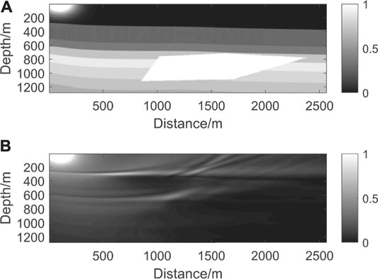
FIGURE 2. Training dataset. (A) is the velocity model with shot information and (B) is the corresponding illumination result calculated by Eq. 2.2.

2.2.2 Network Construction

The UNet network takes the feature information of different scales into account and combines them with each other, so that more features, especially some detailed features are better preserved (Ronneberger et al., 2015). As the illumination is closely related to the subsurface structure, the UNet network was chosen to retain more background geological features. Based on the traditional UNet network, we constructed a network architecture with 6 downsampling layers and upsampling layers. The stride of the pooling layer is 2, and the stride of the convolutional layer is 1. The convolution kernels of the entire network are all the same size as 3x3. The UNet network is show in Figure 3. The final single shot illumination result is obtained through the input of the model with the shot position information at the leftmost.

FIGURE 3

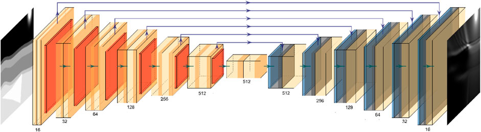
FIGURE 3. Constructed UNet network with 6 downsampling layers.

2.2.3 Training of UNet

In training process, we set the batchsize as 32, and the learning rate lr=0.001 which decreases with the number of training epoch. The data in the constructed dataset is divided into the training dataset and the validation dataset at a ratio of 17:3. The mean square error function is selected as the loss function. The loss function of training dataset is shown in black line of Figure 4. According to the curve trend in Figure 4, the network matches the constructed dataset well, and the parameter selection in training is relatively correct. The abscissa of the graph is the number of training. With the training number increases, the loss value of the validation dataset in red of Figure 4 initially decreases quickly, mainly caused by the mean square error function, and then slowly decreases. For the test dataset, after epoch reaches 30, the value of the loss function tends to be stable.

FIGURE 4

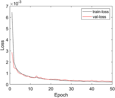
FIGURE 4. Curve of loss function during training (black is training dataset; red is validation dataset).

3 RESULT

We perform trial calculations on the SEG salt dome model with the trained network. The resampled sources start with the location of 1050 m on the surface, and the shot interval is 50 m. The shot is on the right end of the spread. The spread length is 1000 m, and the receiver spacing is 10 m. As shown in Figure 5A, the SEG salt dome model contains a large high-velocity anomaly. Underneath the anomaly, there are complex structures such as folds and faults. It is difficult for the traditional reverse time migration method to obtain a clear geological image globally.

FIGURE 5

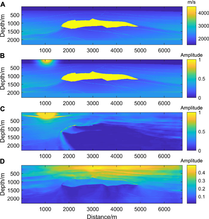
FIGURE 5. (A) is SEG salt velocity model. (B) is the velocity with shot position information and (C) is the Network prediction of single shot illumination result. (D) is the stack of multi-shot one-way illumination results.

The one-way illumination of the seismic source is shown in Figure 5. Figure 5B is the input of the network, and Figure 5C is the single shot illumination result predicted by the network. The average time of calculating a single illumination result by using the regular theory and the deep learning method is 10s and 0.4s, respectively. From Figure 5C, most of the energy propagated from the seismic source is blocked by the high-velocity salt dome. There is a low-energy area below the salt dome. The source has better illumination results above the salt dome. Therefore, it can be preliminarily predicted that the artillery source has strong illumination energy above the salt dome and near the seismic source, and the imaging results also have relatively high resolution in these areas.

Single-shot illumination result can hardly show the overall energy distribution, so we stack all the shots to get full shots illumination in Figure 5D. The overlying stratum above the high-velocity salt dome has strong illumination, and the energy distribution is relatively uniform in the lower left and lower right of the model. The illumination is significantly weak below the high-velocity salt dome. The size of the low illumination area decreases with the distance from the salt dome, and the existence of the salt dome has a key impact on the illumination of the structure below it. According to these predicted illumination results, we believe that the imaging results below the salt dome will have relatively poor quality and low resolution. Without considering whether the geophone can receive the wavefield propagated from the seismic source, the one-way illumination of the seismic source energy does not fit the complete situation of data acquisition well. It is necessary to allow for the receiver impact on the illumination analysis by using Eq. 2.4.

3.1 Determining low illumination area from the target area

According to the one-way illumination result of Figure 5d, we can see the distribution of the low illumination area is relatively wide below the salt body. To be more specified, we manually select an area in Figure 5D as the target area. For example, the box position in Figure 6 is defined as the research area. This area contains fault structures, and it is a challenge for migration to obtain a clear image of this region.

FIGURE 6

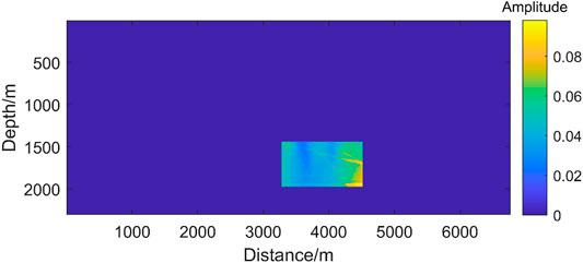
FIGURE 6. The location of target area which is artificially selected according to the illumination result.

In order to further extract the specific location of the low illuminated area in the target area, deep learning can be used to identify the low illuminated area. The dataset used for this model is shown in Figure 7A,B. The upper panel shows the energy illumination of the target area, and the lower one illustrates the marked low illumination area. The marked low illumination area is selected based on the relative average strength in the target area. The total number of training datasets is 1,000*2.

FIGURE 7

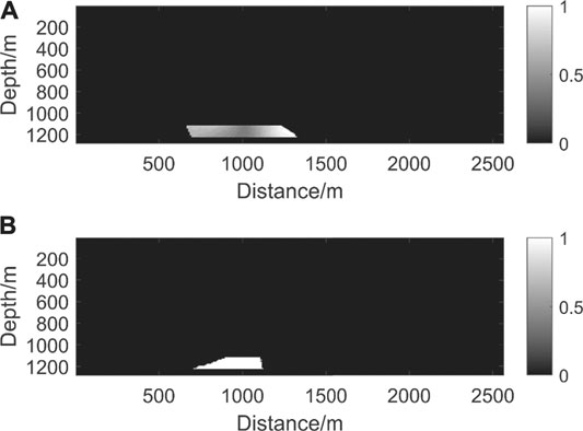
FIGURE 7. Determination of the low illumination area. (A) The illumination results as network input. (B) The picked low illumination area as network output.

In order to fast identify the contour of the low illuminated area in the local area of the picture, a UNet network with three layers of downsampling and three layers of upsampling is constructed. The stride of the pooling layer is 2, and the stride of the convolutional layer is 1. The convolution kernels of the entire network are all the same size as 3*3. The UNet network is show in Figure 8. Considering that the network only needs to further filter the pixel values in the selected target area, it is similar to the recognition of medical images. The input of the network is only the illumination result of the target area, and the output of the network is the position of the identified low illuminated area.

FIGURE 8

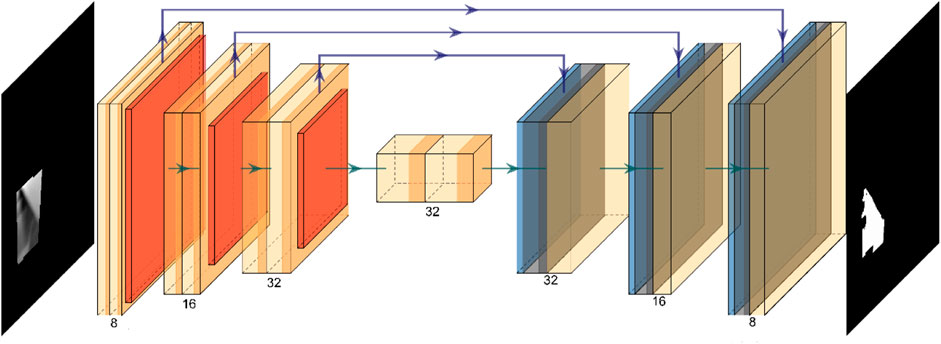
FIGURE 8. Constructed UNet network with 3 downsampling layers.

During network training, the loss function is defined by the root mean square error function. Figure 9 is the loss function curve for network training. It can be seen that the losses of the training and testing are both rapidly decline at the beginning, and after the epoch reaches 20, the value of the loss function tends to be stable.

FIGURE 9

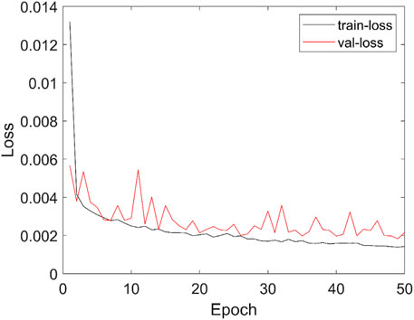
FIGURE 9. Curves of loss function during training (black—training dataset; red—validation dataset).

The stack energy map of one-way or two-way illumination in the target area is input into the trained network model. The result obtained by edge smoothing is shown in the Figure 10A,B (one-way illumination) and Figure 10C,D (two-way illumination), respectively. It can be seen that the weak illumination area is a part of the target area.

FIGURE 10

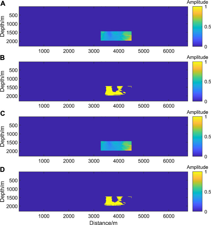
FIGURE 10. The location of low illumination area predicted by the network under the guidance of one-way and two-way illumination. (A) is the target area and (B) is the weak illumination area of one-way illumination. (C) is the target area and (D) is the weak illumination area of two-way illumination.

3.2 Selection of shot based on low illumination area

Based on single-shot illumination results, when its energy intensity of the low illumination area is greater than average, the shot will be kept. By this means we only retain the shots which have dominant contributions on the illumination of the area. The selected shots are successively distributed, and only a few shots are selected separately. For the shot selection results obtained under the two-way illumination situation, the shots are evenly distributed directly above the target area. The shot range is wider, with only one separate shot near the right end. On the whole, the selected shots is about half of the total shot.

3.3 Local imaging based on shot selection

We perform regular reverse time migration for the selected shots above in the target area. In the partial imaging results with one-way illumination in Figure 11A, most of the interface information can be obtained for the restoration of subsurface structures. Due to the constraint of one-way illumination-based shot selection, the results of geological structure imaging in low-illumination areas are clear, while the imaging results of other locations in the target area are relatively poor.

FIGURE 11

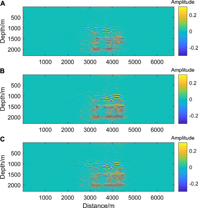
FIGURE 11. (A) is the image result for the target area with shots selected by the one-way illumination. (B) is the image result for the target area with shots selected by the two-way illumination. (C) is the image result for the target area with all shots.

Similarly, the shot gathers selected by the two-way illumination are employed for reverse time migration. In the partial imaging results with two-way illumination in Figure 11B, most of the interface information can be obtained for the restoration of subsurface structures. Compared with Figure 11A, the overall imaging result of the target area is clearer in the non-low illumination area.

We compare the imaging results based on one-way and two-way illumination analysis with the normal all-shots local imaging result as shown in Figure 11C. The approaches with one-way and two-way illumination constraints can recover the subsurface structures very well. The result with one-way illumination is relatively poor in interface continuity, while two-way illumination can overcome this and its imaging result has almost the same accuracy as the all-shots result. The two-way illumination strategy can achieve a balance between accuracy and computational cost.

By comparing the calculation efficiency as shown in Table 1, we see that the local imaging algorithms based on shot selection greatly save the calculation time, and the imaging quality is equivalent to the integrated image results of all shots.

TABLE 1

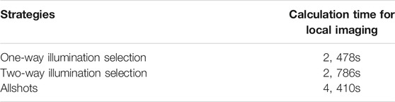
Table 1. Calculation efficiency comparison.

4 DISCUSSION

The illumination analysis based on deep learning provides a preliminary prediction for subsurface seismic energy distribution. According to this, the acquisition system can be optimized to obtain seismic data related to difficult subsurface regions. This method considers various of structures in the training of the network, and can be applied to complex models.

Based on the results of deep learning illumination, we can select the target area to be studied, and further use neural network for the target area to quickly pick out the low illumination area.

By applying the principle of energy intensity filtering to select shot at low illumination area and implement local imaging, the subsurface structures can be imaged well, and the calculation efficiency has also been significantly improved. In the case of 3D model, the number of shots selected by the 3D illumination will be further reduced, and employing the shot selection results for 3D imaging will have a dramatic improvement in computational efficiency compared with regular all-shots imaging.

5 CONCLUSION

The illumination analysis method with deep learning allows us to efficiently compute single-shot illumination results to be employed for shot selection. Compared with the regular wave equation illumination method, the calculation efficiency is significantly improved. By dumping less related shots to the weakly illuminated area, the computational time is reduced furthermore without affecting the imaging quality.

Data Availability Statement

The raw data supporting the conclusions of this article will be made available by the authors, without undue reservation.

Author Contributions

CR programmed with illumination analysis, migration, and deep learning training and prediction; he wrote the manuscript. XJ presented the whole idea and revised the manuscript.

Funding

This study received support from the Joint Open Fund of Mengcheng National Geophysical Observatory (No. MENGO-202005) and the National Natural Science Foundation of China (42074125 & 41774121).

Conflict of Interest

The authors declare that the research was conducted in the absence of any commercial or financial relationships that could be construed as a potential conflict of interest.

Publisher’s Note

All claims expressed in this article are solely those of the authors and do not necessarily represent those of their affiliated organizations, or those of the publisher, the editors and the reviewers. Any product that may be evaluated in this article, or claim that may be made by its manufacturer, is not guaranteed or endorsed by the publisher.

References

Albertin, U., Watts, D., Chang, W., Kapoor, S. J., Stork, C., Kitchenside, P., et al. (2002). Near-salt-flank imaging with Kirchhoff and wavefield extrapolation migration. 72nd SEG Technical Program Expanded Abstracts, 1328–1331. doi:10.1190/1.1816901

CrossRef Full Text | Google Scholar

Baysal, E., Kosloff, D. D., and Sherwood, J. W. C. (1983). Reverse time migration. Geophysics 48, 1514–1524. doi:10.1190/1.1441434

CrossRef Full Text | Google Scholar

Chang, K.-H., Han, M.-H., Roh, J.-K., Kim, I.-O., Han, M.-C., Choi, K.-S., et al. (1990). Gd-dtpa enhanced mr imaging in intracranial tuberculosis. Neuroradiology 32 (1), 19–25. doi:10.1007/bf00593936

PubMed Abstract | CrossRef Full Text | Google Scholar

Chen, B., and Jia, X. (2014). Staining algorithm for seismic modeling and migration. Geophysics 79 (4), S121–S129. doi:10.1190/geo2013-0262.1

CrossRef Full Text | Google Scholar

Chen, S.-C., Ma, Z.-T., and Wu, R.-S. (2007). Illumination compensation for wave equation migration shadow. Chinese J. Geophys. 50 (3), 729–736. doi:10.1002/cjg2.1087

CrossRef Full Text | Google Scholar

Chen, Y. R., Li, Z., Qin, N., and Zhang, K. (2013). Full waveform inversion with wave equation bi-directional illumination optimization. Progress in Geophysics (in Chinese) 28 (006), 3015–3021.

Google Scholar

Claerbout, J. F. (1971). Toward a unified theory of reflector mapping. Geophysics 36 (3), 467–481. doi:10.1190/1.1440185

CrossRef Full Text | Google Scholar

Gray, S. H. (1986). Efficient traveltime calculations for Kirchhoff migration. Geophysics 51, 1685–1688. doi:10.1190/1.1442217

CrossRef Full Text | Google Scholar

Hill, N. R. (1990). Gaussian beam migration. Geophysics 55, 1416–1428. doi:10.1190/1.1442788

CrossRef Full Text | Google Scholar

Jia, Y., and Ma, J. (2017). What can machine learning do for seismic data processing? an interpolation application. Geophysics 82 (3), V163–V177. doi:10.1190/geo2016-0300.1

CrossRef Full Text | Google Scholar

Lecomte, I. (1998). Have a look at the resolution of prestack depth migration for any model, survey and wavefields. 68th SEG Technical Program Expanded Abstracts, 1112–1115. doi:10.1190/1.1820082

CrossRef Full Text | Google Scholar

Liu, Y., Zhang, Z., Zhong, R., Chen, D., Ke, Y., Peethambaran, J., Chen, C., and Sun, L. (2018). Multilevel building detection framework in remote sensing images based on convolutional neural networks. IEEE J. Sel. Top. Appl. Earth Observations Remote Sensing 11, 3688–3700. doi:10.1109/jstars.2018.2866284

CrossRef Full Text | Google Scholar

Mao, J., Wu, R.-S., and Gao, J.-H. (2010). Directional illumination analysis using the local exponential frame. Geophysics 75, S163–S174. doi:10.1190/1.3454361

CrossRef Full Text | Google Scholar

Mauricio, A. P., Jennings, J., Adler, A., and Dahlke, T. (2018). Deep-learning tomography. Leading Edge 37 (1), 58–66.

Google Scholar

McMechan, G. A. (1983). Migration by Extrapolation of Time-dependent Boundary Values*. Geophys Prospect 31, 413–420. doi:10.1111/j.1365-2478.1983.tb01060.x

CrossRef Full Text | Google Scholar

Mulder, W. A., and Plessix, R. E. (2004). A comparison between one‐way and two‐way wave‐equation migration. Geophysics 69, 1491–1504. doi:10.1190/1.1836822

CrossRef Full Text | Google Scholar

Ristow, D., and Rühl, T. (1994). Fourier finite‐difference migration. Geophysics 59, 1882–1893. doi:10.1190/1.1443575

CrossRef Full Text | Google Scholar

Ronneberger, O., Fischer, P., and Brox, T. (2015). U-net: convolutional networks for biomedical image segmentation. LNCS 9351, 234–241. doi:10.1007/978-3-319-24574-4_28

CrossRef Full Text | Google Scholar

Stolt, R. H. (1978). Migration by fourier transform. Geophysics 43 (1), 23–48. doi:10.1190/1.1440826

CrossRef Full Text | Google Scholar

Sun, J., Wang, D. L., Wang, T., Zhang, Y. B., Wang, T. X., and Tian, M. (2018). Study of multiples illumination analysis method based on two-way wave equation. Progress in Geophysics 033 (001), 243–249.

Google Scholar

Vigh, D., Jiao, K., Cheng, X., Sun, D., and Lewis, W. (2016). Earth-model building from shallow to deep with full-waveform inversion. The Leading Edge 35 (12), 1025–1030. doi:10.1190/tle35121025.1

CrossRef Full Text | Google Scholar

Wu, W. J., Lines, L. R., and Lu, H. X. (1996). Analysis of higher‐order, finite‐difference schemes in 3-D reverse‐time migration. Geophysics 61 (3), 845–856. doi:10.1190/1.1444009

CrossRef Full Text | Google Scholar

Xie, X. B., Jin, S, and Wu, R. S. (2003). Three-dimensional illumination analysis using wave equation based propagator. 73rd SEG Technical Program Expanded Abstracts, 989–992.

Google Scholar

Xie, X. B., He, Y. Q., and Li, P. M. (2013). Seismic illumination analysis and its applications in seismic survey design. Chinese Journal of Geophysics-Chinese Edition 56 (5), 1568–1581.

Google Scholar

Yan, Z., and Xie, X.-B. (2016). Full-wave seismic illumination and resolution analyses: A Poynting-vector-based method. Geophysics 81, S447–S458. doi:10.1190/geo2016-0003.1

CrossRef Full Text | Google Scholar

Yang, H., Xie, X. B., Luo, M., and Jin, S. (2008). Target oriented full-wave equation based illumination analysis. 78th SEG Technical Program Expanded Abstracts, 2216–2220. doi:10.1190/1.3059326

CrossRef Full Text | Google Scholar