Groundwater Drought and Cycles in Xuchang City, China

Introduction

Drought is an extreme and complex natural disaster that can cause great economic losses and has the characteristics of long duration, wide impact, and high frequency. It seriously threatens the safety and stability of human society and is called a “spreading disaster” (Mishra and Singh, 2010; Wilhite, 2000). Climate change has a huge impact on hydrological processes (Intergovernmental Panel on Climate Change (IPCC), 2013; Wilhite, 2000; Oo et al., 2020), and its impact on groundwater resources cannot be ignored (Zhou et al., 2010; Kavitha and Chandran, 2015; Dua et al., 2020). Groundwater drought, as a concept that links groundwater resources with drought, is gradually separating from hydrological drought and agricultural drought and has become a separate research area in recent years, gaining the attention of scholars from around the world. It is defined as a phenomenon in which the groundwater level is lower than the normal or the flow rate decreases in the spring (Van Loon and Anne, 2015; Marchant and Bloomfield, 2018). Like other common droughts, it is a natural disaster caused by the dual impact of social development and climate change, impeding the development and stability of society (Taylor et al., 2012; Medellín-Azuara et al., 2015). Natural factors causing such droughts include temperature and precipitation. Rising temperatures lead to an increase in evapotranspiration, and insufficient precipitation leads to a decrease in surface runoff and soil moisture, thus affecting groundwater replenishment. In addition, a large amount of groundwater is used for intensive farmland irrigation, and a small amount of groundwater is used in households and production. Overexploitation of groundwater makes it difficult for groundwater to return to normal levels, leading to groundwater drought. The pressure, state, and response of the groundwater drought are shown in Figure 1.

FIGURE 1

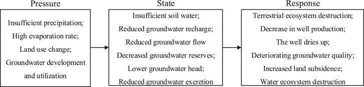
FIGURE 1. Schematic diagram of groundwater drought pressure, state, and response.

Under the combined influence of natural factors and human activities, groundwater drought may exhibit complex characteristics. In addition, due to the lack of direct observational data on groundwater resources, it is difficult to quantitatively assess groundwater drought. However, since groundwater drought has attracted the attention of scholars in the fields of meteorology, hydrology, and geology, it has become an important research topic. The Groundwater Resource Index (GRI), as a reliable tool in a multi-analysis approach for monitoring and forecasting drought conditions, was developed by Mendicino et al. (2008). Macdonald et al. (2009) studied the principles of groundwater drought using hydrogeological maps, while Li and Rodell (2015) used the Groundwater Drought Index (GWI) to assess groundwater drought in the central and northeastern United States. After the launch of the Gravity Recovery and Climate Experiment (GRACE) satellite, scholars will be able to use remote sensing methods to assess changes in groundwater reserves and use the results in response to drought (Scanlon BR. et al., 2012; Scanlon B. R. et al., 2012). Until 2017, Thomas et al. (2017) explicitly included and evaluated the Groundwater Drought Index based on GRACE observations to understand and identify groundwater drought and applied it in the Central Valley of California, thus pioneering the direct application of the GRACE satellite to assess groundwater drought. Seo and Lee (2019) combined GRACE satellite data and other remote sensing methods to build an artificial neural network model to monitor the groundwater drought in South Korea, thus providing a new idea for the use of satellite methods to monitor groundwater drought. Wang et al. (2020) used the GRACE Groundwater Drought Index (GGDI) as an indicator to assess groundwater drought and comprehensively identified the temporal evolution, spatial distribution, and trend characteristics of the drought in the North China Plain from 2003 to 2015. Afterwards, they used cross-wavelet transform technology to clarify the difference between GGDI and teleconnection factors. The relationship between relevant factors has achieved good results and gained new insights for the application of GRACE gravity satellites to monitor groundwater drought. The Standardized Water-Level Index (SWI) was originally developed by Bhuiyan (2004) to evaluate the hydrological drought with the help of the groundwater level recharge deficit and was later applied to the study of groundwater drought. Rahim et al. (2015) used SWI to estimate the groundwater recharge deficit in the pre-monsoon and post-monsoon seasons and then performed a spatial interpolation to determine the degree of groundwater drought in the study area. Nagarajan et al. (2015) used SWI as a Ground Observation Index combined with satellite information to evaluate the drought vulnerability of the Peddavagu watershed in the sub-basin of the Krishna River system on the Indian peninsula.

The Standardized Precipitation Index (SPI) is one of the most widely used evaluation indicators in the field of drought. Monitoring meteorological droughts can serve as a guide for planning and implementing groundwater management policies (CTGCD, 2011; Texas Water Code, 2016). Therefore, it is also used in the assessment of groundwater drought (Fiorillo and Guadagno, 2010; Fiorillo and Guadagno, 2012). Bhuiyan et al. (2006) combined SWI with SPI, Normalized Difference Vegetation Index (NDVI), Vegetation Condition Index (VCI), Temperature Condition Index (TCI), and Vegetation Health Index (VHI) to monitor drought dynamics in the Alawari region (India). On the basis of SPI, Bloomfield Marchant (2013) and Bloomfield et al. (2015) used monthly groundwater level data to construct the Standardized Groundwater-Level Index (SGI), which is specifically used to evaluate groundwater drought, and analyzed the correlation between SGI and SPI on multiple time scales. As a result, the use of SGI to assess groundwater drought has grown. Pathak et al. (2016) performed a cluster analysis of the long-term monthly groundwater level in the Gataprabha River Basin in India. This study classified observation wells which performed the Mann-Kendall test in order to analyze annual and seasonal groundwater level trends and used SGI to evaluate the area groundwater drought. Motlagh et al. (2016) used stochastic models to predict the groundwater level and then used SGI to predict and warn the local groundwater drought. Liu et al. (2016) used monthly groundwater level data from 40 observation wells in Jiangsu Province, China, from 1989 to 2012, and used SGI to conduct a spatio-temporal analysis of groundwater drought in the province. However, the calculation method of SGI proposed by Bloomfield Marchant (2013); Bloomfield et al. (2015) considered both parametric and non-parametric cases. The monthly series of groundwater level were fitted with the gamma function, without considering whether the gamma function could be fitted with the monthly series data of groundwater level in other regions, which would have a certain impact on the final groundwater drought assessment. Based on this, Lorenzo-Lacruz et al. (2017) modified the SGI according to the Standardized Runoff Index (SSI) (Vicente-Serrano et al., 2012) and established an index according to different probability distributions of monthly series of groundwater level, which can ensure adaptability of calculated SGI to different climate and water conditions and can more accurately reflect the conditions of groundwater drought.

Drought monitoring and identification of characteristics are an important part of dealing with drought risks (Harisuseno, 2020; Kavianpour et al., 2020). Based on a quantitative assessment of groundwater drought conditions, some scholars have begun to identify the characteristics of groundwater drought. Groundwater drought has characteristics similar to traditional drought, which is a multivariate phenomenon. There is a certain correlation and dependence between several characteristic variables (e.g., drought duration, drought intensity, and drought influence range), so traditional analysis with one variable (e.g., drought frequency) may not be conducive to comprehensively study groundwater drought events, leading to insufficient and inaccurate drought risk assessment (Pathak and Dodamani, 2021). The Copula function has been widely used in drought field research (Zhou et al., 2012; Xu et al., 2015; Wu et al., 2018). It can fit into the distribution functions of multiple drought-characteristic variables and can effectively describe the correlation between variables. Although groundwater drought research started late, studies have shown that the Copula function can also be used in research and analysis of groundwater drought. For example, while Saghafian and Sanginabadi (2020) proposed a framework for statistical analysis of disturbed hydrological system, they carried out multivariate groundwater drought analysis based on the Copula function in an overexploited aquifer and used a goodness-of-fit test to compare Copula and the empirical groundwater drought frequency, which proved that the Copula model had sufficient accuracy in multivariate drought analysis. Pathak and Dodamani (2021) studied the response of groundwater drought to meteorological drought and the local aquifer characteristics using monthly groundwater level data in the tropical river basin of India and the Copula function to conduct a bivariate (drought intensity and drought duration) frequency analysis of groundwater drought.

However, research on the characteristics of groundwater drought is mainly concentrated in the return period (frequency analysis), and there is little research on the groundwater drought cycle. The return period is the frequency of events in a certain period, which is random and uncertain, and the drought return period is mainly used to evaluate the severity of drought events. A cycle is a cyclic law that exists in the development process of things, which is deterministic, and the drought cycle is the time interval between two adjacent droughts. Therefore, conducting research on the groundwater drought cycle can provide a more comprehensive understanding of groundwater drought characteristics, understand the law of regional groundwater development, and strengthen the groundwater drought early warning mechanism. Continuous wavelet transform is a common method in wavelet analysis. It can more effectively identify the non-monotonic trend of hydrological sequences (Sang et al., 2018) and is widely used in the field of hydrology. For example, Pathak et al. (2016) used wavelet transform methods to analyze seasonal temperatures, precipitation, and runoff trends in the Midwest of the United States. Djordje et al. (2021) used wavelet transform spectrum analysis (WTS) and other methods to study the long-term characteristics of the Danube water level and the flow and changes in natural cycles. Palizdan (2017) applied a continuous wavelet transform to analyze the long-term precipitation trend in the Langat River Basin (Malaysia), while Li and Zhu (2021) further improved the wavelet transform method to identify the runoff cycle of the Heihe River (China).

In this paper, we used the continuous wavelet transform method to identify the period of groundwater drought and to grasp the principles of groundwater drought in Xuchang city. The objectives of this study are 1) to determine changes in groundwater drought in different observation wells in Xuchang city from 1980 to 2018 and 2) to evaluate the change cycle of groundwater drought in Xuchang city.

Data and Methods

Study Area

Xuchang city (34°16′–34°58′N, 112°42′–114°14′E) is located in the central part of Henan Province (China) and covers an area of 4,996 km². It is located in the transition zone between Funiu Mountain and the Eastern Henan Plain. Plains dominate with 72.8%, while hills and mountains account for 16.8 and 10.4%, respectively. The region has a temperate continental monsoon climate with an average annual temperature from 14.3 to 14.6°C and an average annual precipitation from 671 to 736 mm. According to the lithological characteristics of aquifers and the nature of groundwater storage in Xuchang area, regional groundwater can be divided into four types: loose rock pore water, clastic rock fissure water, carbonate rock fissure karst water, and magmatic rock fissure water. Pore water is distributed in vast plains and hilly areas, whereas fissure water and karst water are distributed in the bedrocks of the mountains. The shallow loose rock-type pore is the most important water-bearing rock group in the region and the analyzed groundwater belongs to this group.

Data

Monthly groundwater level data were obtained from the local Hydrographic Bureau. We used the monthly data from seven observation wells with relatively complete datasets from 1980 to 2018. For some missing data, cubic spline function interpolation was used to supplement the data (Peng-zhu et al., 2015). The locations of the seven observation wells are shown in Figure 2.

FIGURE 2

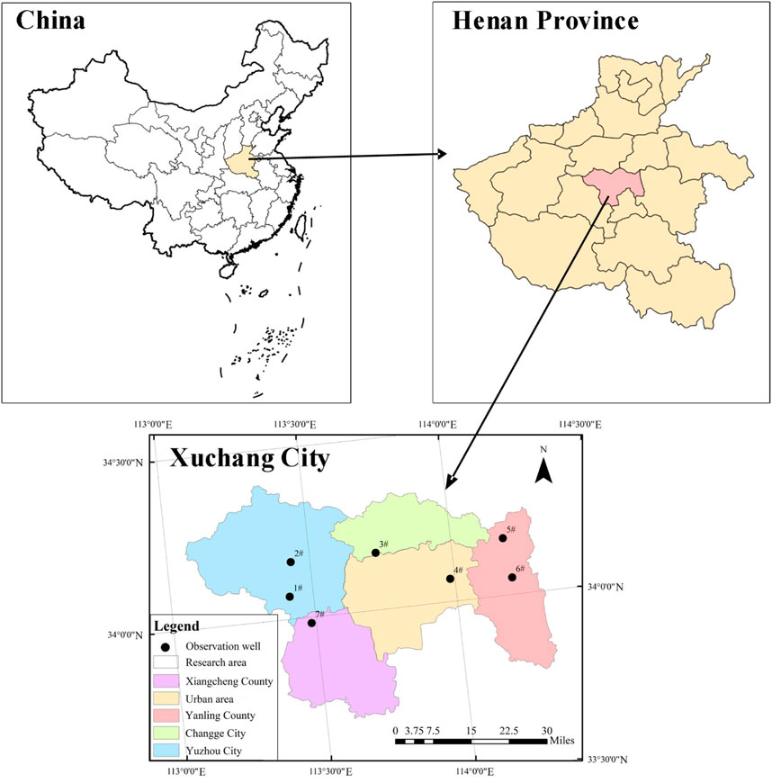
FIGURE 2. Location of the study area and the seven observation wells.

Methods

Standardized Groundwater Index

The SGI is an indicator that measures the degree of groundwater drought based on changes in groundwater level. It is currently a more reliable tool for assessing groundwater drought. Bloomfield et al. (2015) revised the Standardized Precipitation Index (SPI) and proposed the SGI for groundwater drought analysis. In their study, the SGI uses gamma distribution in SPI for fitting. However, the monthly distribution of groundwater may not be consistent with the gamma distribution (Liu et al., 2016), and therefore the method proposed by Lorenzo-Lacruz et al., 2017 can be used to calculate SGI for different fitting distribution functions in this study. The SGI calculation formula (Lorenzo-Lacruz et al., 2017) is as follows:

$SGI=S\left(\text{W}-\frac{C_0+C_{1}W+C_2{W}^2}{1+d_{1}W+d_2{W}^2+d_3{W}^3}\right),(1)$

$W=\sqrt{-2\ln P},(2)$

where F(x) is the cumulative distribution probability for determining the fitted distribution function, P is the groundwater level distribution probability related to function F(x), x is the monthly groundwater level sample, and S is the positive and negative coefficient of probability density. If F(x) ≥ 0.5, P = 1-F(x), S = 1; if not, P = F(x), S = −1. C₀, C₁, C₂ and d₁, d₂, d₃ are the calculation parameters of the gamma distribution function converted into cumulative frequency in order to simplify the approximate solution formula. The constants are C₀ = 2.515517, C₁ = 0.802853, C₂ = 0.010328, d₁ = 1.432788, d₂ = 0.189269, and d₃ = 0.001308.

Based on this, the key to calculating the SGI is to find the most suitable fitting distribution function. Here, we used gamma distribution, beta distribution, log-normal distribution (logN), Weibull distribution (Web), normal distribution, and the generalized extreme value (GEV) distribution to fit the data of the seven observation wells. These distribution functions are not only more common but also have strong adaptability, satisfying the cumulative frequency calculation of monthly data series on groundwater levels in different situations (Guttman, 1998).

Prior to calculating the SGI, we normalized the original data column ($\text{x}$) and introduced the processed data column ($\text{x'}$) in subsequent calculations. To facilitate subsequent distribution function fitting, we replaced 0 and 1 in the new data column with 0.001 and 0.999, respectively. The normalization formula (Chen et al., 2019) is as follows:

$x\prime =\frac{\max \left(x\right)-x}{\max \left(x\right)-\min \left(x\right)}.(3)$

After obtaining a normalized data column, we began to fit the distribution function. This step was performed with the help of the MATLAB 2018b software platform.

After that, the Kolmogorov–Smirnov (KS) test was performed on the fitting distribution results of the data of each observation well, and the fitting distribution function with the lowest statistic D was selected as the best fitting distribution function of the observation well, introduced into Eq. 1. The KS test equation (Xi-zhi and Wang, 1996) is as follows:

$D=\max \left({\max }_i\left|COF\left(x_i\right)-\frac{r-1}{n},\frac{r}{n}-CDF\left(xi\right)\right|\right),(4)$

where r is the rank of the observation i in ascending order.

Wavelet Analysis

Wavelet analysis, known as the “mathematical microscope,” is particularly suitable for processing non-stationary signals because it can detect the characteristics of time-frequency detailed information and can reveal the main distribution of oscillation periods hidden in time series, which is useful for the future of the system. The development trend has been qualitatively estimated and is widely used in the research fields related to atmosphere, hydrology, and geography, among others (Aussen et al., 1997; Smith et al., 1998; Nason and Sapatinas, 2002).

When using wavelet to analyze practical problems, we have to choose the suitable basis for the wavelet function. Morlet is a harmonic smoothed by the Gaussian function and a complex wavelet that is widely used in the field of hydrology (Kulkarni, 2000). Therefore, we chose Morlet’s continuous complex wavelet transform to analyze the characteristics of groundwater time series on multiple time scales. For a given wavelet function, continuous wavelet transform of the hydrological time series $f\left(t\right)\in L^2\left(R\right)$(Wang et al., 2005) is expressed as follows:

$W_f\left(a,b\right)={\left|a\right|}^{-\frac{1}{2}}{\displaystyle {\int }_{-\infty }^{\infty }f\left(t\right)\overline{\psi }\left(\frac{t-b}{a}\right)}dt,(5)$

where $a$ is the scaling scale ($a\ne 0$), which reflects the characteristics of the frequency domain; b is the translation parameter, which reflects the characteristics of the time domain; $\overline{\psi }\left(\frac{t-b}{a}\right)$ is the complex conjugate function of $\psi \left(t\right)$; and $\overline{\psi \left(t\right)}$ is the basis wavelet function. Here, $W_f(a,b)$ is the wavelet transform coefficient, which is the inner product of the continuous wavelet and the signal on the scale $a$ and displacement b, indicating the degree of similarity between the signal and the wavelet represented by the point. When the value of $a$ is small, a higher time domain resolution can be obtained; the opposite occurs for small value of $a$.

Because it is difficult to express a continuous sequence with digital symbols in actual application, a continuous time sequence is often discretized. This is also the case for hydrological time series. Total, average, or extreme values of the process state are often used as time series values, such as precipitation, water level, and runoff (Wu, 2014).

The discrete form of wavelet transform (Hou and Wang, 2011) is expressed as follows:

$W_f\left(a,b\right)={\left|a\right|}^{-\frac{1}{2}}\Delta t{\displaystyle {\sum }_{k=1}^{N}f\left(k\Delta t\right)}\overline{\psi }\left(\frac{k\Delta t-b}{a}\right),(6)$

where $W_f(a,b)$ is a function that varies depending on the parameters $a$ and $b$. Since the Morlet wavelet is a complex number, the transformed coefficients are also complex numbers. We took the real part of the wavelet coefficients, namely,$b$ as the abscissa and $a$ as the ordinate, in order to generate a two-dimensional contour map of $W_f(a,b)$, i.e., the contour plot of the real part of the wavelet coefficients.

When the scale $a$ is the same, the process of changing the wavelet transform coefficients over time reflects the characteristics of the change of the hydrological time series on this scale: when the wavelet transform coefficient is greater than 0, it is in the multi period; when the wavelet transform coefficient is less than 0, it is in the minor period. Similarly, when the wavelet transform coefficient is 0, it is in the transition stage from minor to multi period or from multi to minor period (Hou and Wang, 2011).

By integrating the square value of the wavelet coefficient in the time translation domain (b), the wavelet variance $\text{Var}$ (Cahill, 2002; Kang et al., 2009) can be obtained:

$Var\left(a\right)={\displaystyle {\int }_{-\infty }^{\infty }{\left|W_f\left(a,b\right)\right|}^{2}db}.(7)$

The discrete form is expressed as follows:

$Var\left(a\right)=\frac{1}{N}{\displaystyle {\sum }_{t=1}^N{\left|W_f\left(a,x_t\right)\right|}^2},(8)$

where $Var\left(a\right)$ is the wavelet variance; $N$ is the length of the groundwater level data column; and $W_f(a,x_t)$ is the square of the wavelet coefficients on the scale $a$ and time $x_t$, and it is the square of the coefficient modulus for complex coefficients.

The distribution diagram of the $\text{Var}$ change during the period $a$ is called the “wavelet variance distribution diagram” and can intuitively reflect the energy distribution of the signal fluctuation with the period $a$, determining the relative intensity of the different oscillation periods and the main oscillation period.

Results

Selection of the Best Fit Function

As mentioned above, the key to SGI calculation is to select the fitting function. We used six more common functions to fit the data series from the seven observation wells and performed the KS test (Eq. 4) on the fitting results; finally, we chose the function with the lowest test statistic D as the best fit function for the SGI calculation (Cui et al., 2020).

Table 1 shows that the best fitting distribution function for the well-1#, well-2#, well-5#, and well-7# is the GEV function, that for the well-3# is the gamma function, and that for the well-4# and well-6# is the beta function.

TABLE 1

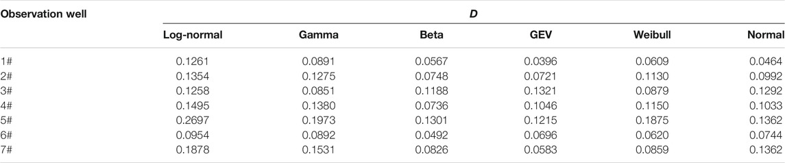
TABLE 1. Results of the Kolmogorov–Smirnov test for seven wells.

SGI Sequence Characteristics

We used Eq. 1 to calculate 3,276 Standardized Groundwater Index values of monthly series of groundwater level from 1980 to 2018 for all observation wells. When SGI <0, drought occurs; when SGI = 0, the well is in a critical state; and when SGI >0, the conditions are normal. Here, we defined continuous drought (i.e., drought duration t ≥ 2 months) as a drought event. The results show (Figure 3) that drought and non-drought occurred alternately in all observation wells, albeit at different intervals. Except for well-5#, the alternating drought and non-drought trends for the remaining six wells were similar, whereas those for well-5# showed the opposite pattern. In addition, the overall trend of the average SGI sequence curve was most similar to that of well-4#.

FIGURE 3

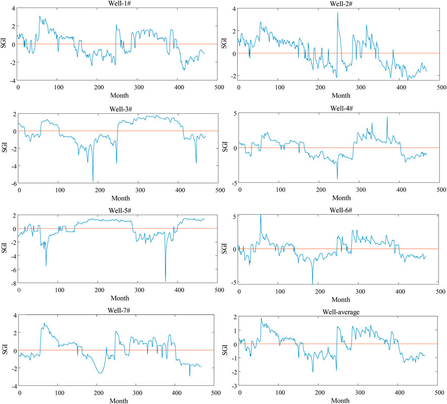
FIGURE 3. SGI time series values.

The number of drought events in the seven observation wells was from 3 to 11, the total drought duration was from 210 to 242 months, the maximum drought intensity was from 104.40 to 187.10, and the longest duration of drought events was from 67 to 146 months. Well-3# had the least drought events, which was three times. However, due to the drought duration, drought intensity, and drought severity characteristics, well-3# faced the most severe drought. Short-term drought often occurs in well-1# and well-6#. The drought intensity in well-7# is the weakest and the duration of the maximum drought event is the shortest. The total duration of drought is the shortest in well-4#. Detailed characteristics of the SGI sequence of the seven observation wells are shown in Table 2.

TABLE 2

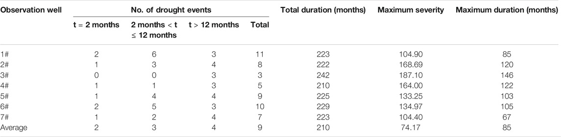
TABLE 2. Drought characteristics based on SGI values for seven observation wells.

Interannual Variation of Groundwater Drought

Because groundwater drought is a cumulative condition, we used the SGI in December each year to represent the groundwater drought in that year. Figure 4 shows the interannual variations of groundwater drought in the seven observation wells of nearly 39a (1980–2018) in Xuchang city (color represents SGI value). Groundwater drought in well-1#, well-2#, and well-4# occurred in 17 years. The strongest droughts occurred in 2014, 2015, and 1999. The coverage period of well-3# groundwater drought was 20 years, and the strongest drought occurred in 2016. Well-5# groundwater had the longest drought coverage period of 21 years, and the strongest drought occurred in 1985. The drought coverage period of well-6# was 19 years, and the strongest drought occurred in 1993. The well-7# groundwater drought coverage period was 18 years, and the strongest drought occurred in 1996.

FIGURE 4

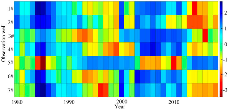
FIGURE 4. Interannual variation of groundwater drought for all seven wells.

Interestingly, the drought years of well-5# were basically spaced apart from those other six. When excluding well-5#, there were no groundwater droughts in the periods 1984–1987 and 2003–2008. In 1994, 1996–1999, and 2014–2018, droughts were observed in other six wells, while no groundwater drought was observed for well-5# during this period.

Characteristics of Groundwater Drought Cycle

In this paper, the 39a regional groundwater SGI sequence was used for wavelet transformation. In this step, we used the MATLAB wavelet toolbox to complete the wavelet transformation graph. We took the real part of the wavelet coefficients, the number of months as the abscissa (e.g., the abscissa 100 in Figure 5 represents the 100th month) and the time scale as the ordinate, and drew the contour plot of the real part of the wavelet coefficients (Figure 5). To more intuitively understand the periodic changes of groundwater drought, the depth of color in Figure 5 represents the size of the real part of the wavelet coefficient. The darker the color, the smaller the SGI value and the stronger the groundwater drought; the lighter the color, the greater the SGI value and the less severe the groundwater drought. Wavelet coefficients change characteristics can be used to characterize SGI time series change characteristics: when the real part of the wavelet coefficient is greater than 0, i.e., the SGI is greater than 0, there is no groundwater drought; when the real part of the wavelet coefficient is less than 0, i.e., the SGI is less than 0, there is groundwater drought. When the real part of the wavelet coefficient is 0, that is, SGI is equal to 0, it represents a turning point in the groundwater transition from drought to non-arid conditions or from non-arid conditions to drought.

FIGURE 5

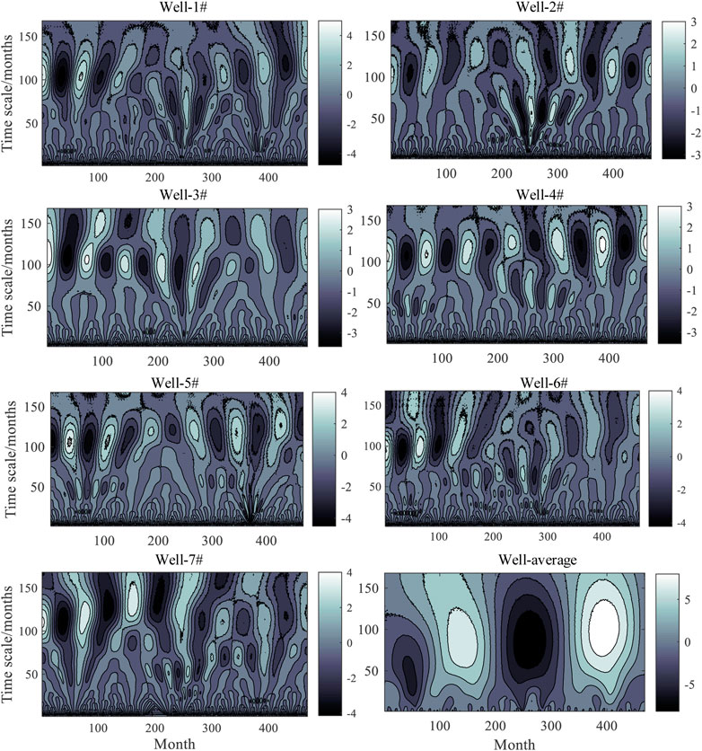
FIGURE 5. Contour plot of the real part of the wavelet coefficients.

The wavelet variance chart can reflect the distribution of the SGI time series fluctuation amplitude with the scale $a$ and can be used to identify the intensity of disturbances and periodic changes at various scales, thereby determining the main period in the evolution of groundwater drought. We calculated the wavelet variance of the SGI time series of all observation wells according to Eq. 8 and drew a wavelet variance graph (Figure 6) with the time scale $a$ as the abscissa and the wavelet variance as the ordinate.

FIGURE 6

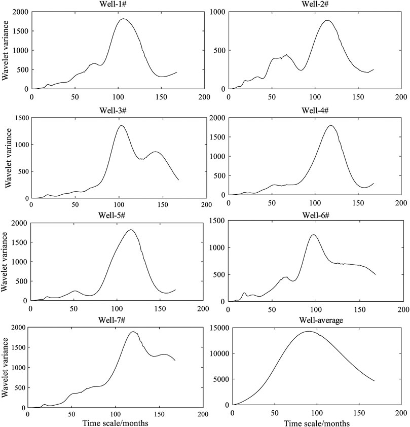
FIGURE 6. Wavelet variance map.

According to the results of the wavelet variance calculation, drawing a real part processing line diagram of the wavelet coefficients in the first and second main periods (Figure 7) can help understand the impact of the two main periods on groundwater drought throughout the study period. Usually, in the same period, the larger the amplitude of the wavelet coefficient real part processing line, the greater the influence in this period, that is, the period is dominated by the variation of the main period.

FIGURE 7

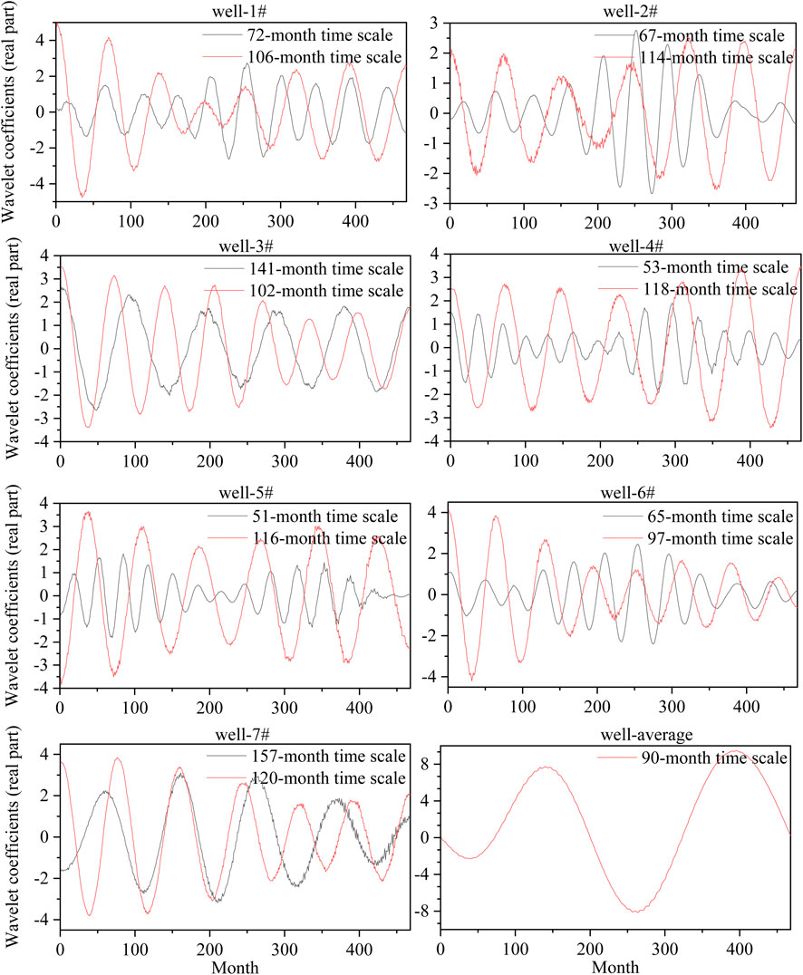
FIGURE 7. Real part of the wavelet coefficient of groundwater drought time scale in the first two main periods.

According to the results of the wavelet analysis, the characteristics of the groundwater drought oscillation period in seven observation wells can be obtained (Table 3). It can be seen from the table that there are 2–4 types of time scale laws in all observation wells, and different types of time scale laws correspond to different main periods. This paper analyzes only the first and second main periods that can best represent the characteristics of the groundwater drought oscillation cycle in each well. The first major period of groundwater drought in the seven observation wells was concentrated between 97 and 120 months, i.e., between 8 and 10 years. Apart from the fact that the second main period of well-3# and well-7# is longer than the first main period, the second main period of other wells basically fluctuates up and down half of the first main period. As can be seen from Figure 6, small cycles are included in the large cycles. As for the situation of well-3# and well-7#, it is very likely that the length of data is not enough, which leads to a larger main period not being found, but according to the size of the first and second main periods of other observation wells, we speculate that the actual first main period of the two wells is twice as long as the existing first main period. However, due to the influence of the data, we can only roughly conclude that the first major periods of the two wells are 102 and 120 months, respectively. There is one type of time scale rule of the average SGI time series and it corresponds to a single main period (90 months), which is 20 months away from the average first main period (110 months) of each well.

TABLE 3

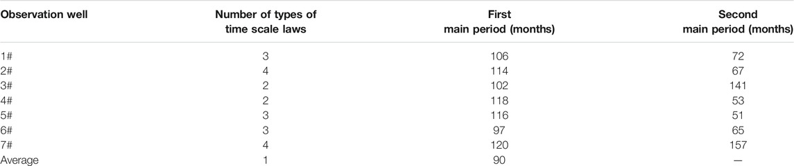
TABLE 3. Period characteristics of groundwater drought oscillation.

Discussion

Climate change and human activities are the main factors causing changes in groundwater levels (Dua et al., 2020; Kavitha and Chandran, 2015; Zhou et al., 2010), and in this study, the Groundwater Drought Index SGI is based on groundwater level data. So, the response of well-5# to changes in the environment differs from those of the other observation wells, most likely due to factors. Due the lack of data, we could not investigate this basic mechanism in more depth. However, it is now clear that conventional droughts can spread faster to groundwater droughts in areas that respond faster to factors.

Drought periods in the seven observation wells differed up to 23 months. Since all these observation wells contain shallow loose rock pore water, there is no difference in the lithology of the aquifer. Therefore, we believe that this difference may be due to regional climate change and human activities. In this sense, the definition of the impact on groundwater drought requires further analysis.

The second main periods of well-3# and well-7# were both longer than the first main period, and in Figure 5, the contours on the second main cycle time scale of these two wells are not closed. However, the unclosed contour loop had a closed trend. It is necessary to confirm whether the cycle of groundwater drought change of the two wells will have a higher periodicity in a certain period of time in the future.

Morlet wavelet transform analysis showed that the groundwater drought period in Xuchang city is 110 months, which is about 9 years. Previous studies have shown that drought periods are closely related to solar activity, and a small period of solar activity is 10 years (Li et al., 2015, Li et al., 2019), which is basically consistent with the results of this study (the subtle difference may be caused by human activities). Therefore, Morlet’s continuous complex wavelet transform can be used to study the groundwater drought cycles. Our results provide a scientific basis for improved groundwater management.

Conclusion

Drought events occurred in all seven observation wells, of which the number of occurrences was the lowest in well-3#, but the drought was the worst. Well-1# has the highest number of drought events, but is dominated by short-lived droughts. Well-4# has the shortest total drought duration, and well-7# has the lowest drought intensity and the shortest duration of the longest drought event. The maximum drought intensity in the seven observation wells is between 104.40 and 187.10.

The drought years of all observation wells were 17–21 years, and the drought years of well-5# were basically spaced apart from other six. The drought years of well-5# are concentrated in periods 1984–1987 and 2003–2012, while the drought years of other observation wells were concentrated in periods 1994–1999 and 2014–2018.

The contour map of the real part of the wavelet coefficients of each well showed a clear quasi-lateral, positive and negative interlaced closed center, distributed from low frequency to high frequency, which indicates an obvious period of oscillation for groundwater drought in Xuchang city. Wavelet transform analysis shows that the groundwater drought period of the seven observation wells was concentrated between 97 and 120 months, i.e., between 8 and 10 years. The groundwater drought period in well-7# was the longest with 120 months, and that of well-6# was the shortest with 97 months. Moreover, each observation well had a second main cycle of different sizes, indicating that the main periods of groundwater drought oscillations are different in different time periods. In addition, we infer that the time scale difference between the first and second main period is basically half of the first main period, and the change law of the small-time scale is included in the large time scale.

Wavelet analysis of the average SGI time series of the seven observation wells shows that the groundwater drought period (90 months) differed considerably from the average period of each well (approximately 110 months), indicating that the average SGI time series of the seven wells is not available. The results of the wavelet analysis can be used to determine the overall groundwater drought cycle in the region.

Data Availability Statement

The data analyzed in this study are subject to the following licenses/restrictions: obtain the approval of the local hydrological department; requests to access these datasets should be directed to http://slj.xuchang.gov.cn/.

Author Contributions

JH, LHC, and FRY contributed to conception and design of the study. LW organized the database. XBL performed the statistical analysis. JH wrote the first draft of the manuscript. JH, LHC, and FRY wrote sections of the manuscript. All authors contributed to manuscript revision, read, and approved the submitted version.

Funding

This research was supported by the Henan Province (China) Water Conservancy Science and Technology Project. Groundwater data were provided by the Xuchang city (China) Hydrological Bureau.

Conflict of Interest

The authors declare that the research was conducted in the absence of any commercial or financial relationships that could be construed as a potential conflict of interest.

Publisher’s Note

All claims expressed in this article are solely those of the authors and do not necessarily represent those of their affiliated organizations, or those of the publisher, the editors, and the reviewers. Any product that may be evaluated in this article, or claim that may be made by its manufacturer, is not guaranteed or endorsed by the publisher.

References

Aussen, A., Campell, J., and Murtagh, F. (1997). Wavelet Based Feature Extraction and Decomposition, Strategies for Financial Forecasting [J]. J. Comput. Intelligence Finance. 6 (2), 5–12.

Google Scholar

Bhuiyan, C. (2004). “Various Drought Indices for Monitoring Drought Condition in Aravalli Terrain of India,” in XXth ISPRS Congress, Istanbul, Turkey, July 12–23, 2004.

Google Scholar

Bhuiyan, C., Singh, R. P., and Kogan, F. N. (2006). Monitoring Drought Dynamics in the Aravalli Region (India) Using Different Indices Based on Ground and Remote Sensing Data. Int. J. Appl. Earth Observation Geoinformation 8 (4), 289–302. doi:10.1016/j.jag.2006.03.002

CrossRef Full Text | Google Scholar

Bloomfield, J. P., and Marchant, B. P. (2013). Analysis of Groundwater Drought Building on the Standardised Precipitation index Approach. Hydrol. Earth Syst. Sci. 17 (12), 4769–4787. doi:10.5194/hess-17-4769-2013

CrossRef Full Text | Google Scholar

Bloomfield, J. P., Marchant, B. P., Bricker, S. H., and Morgan, R. B. (2015). Regional Analysis of Groundwater Droughts Using Hydrograph Classification. Hydrol. Earth Syst. Sci. 19 (10), 4327–4344. doi:10.5194/hess-19-4327-2015

CrossRef Full Text | Google Scholar

Cahill, A. T. (2002). Determination of Changes in Streamflow Variance by Means of a Wavelet-Based Test. Water Resour. Res. 38 (6), 1. doi:10.1029/2000wr000192

CrossRef Full Text | Google Scholar

Chen, H., Zhang, Y., Qi, H., and Li, D. (2019). Detection of Ethanol Content in Ethanol Diesel Based on PLS and Multispectral Method. Optik 195, 162861. doi:10.1016/j.ijleo.2019.05.067

CrossRef Full Text | Google Scholar

CTGCD (2011). Central Texas Groundwater Conservation District -Drought Management Plan. Burnet, TX: Central Texas Groundwater Conservation District, 4.

Cui, Y., Yongfu, W., Xu, X. M., and Liu, J. P. (2020). Groundwater Level Dynamics and its Response to Variations of Precipitation Based on Standardized Groundwater Index[J]. Sci. Tech. Eng. 20 (16), 6336–6342. doi:10.3969/j.issn.1671-1815.2020.16.004

CrossRef Full Text | Google Scholar

Djordje, S., Ilija, B. B., Vladimir, D., and Suzana, B. (2021). Changes in Long-Term Properties and Natural Cycles of the Danube River Level and Flow Induced by Damming[J]. Physica A: Stat. Mech. its Appl. 566, 125607. doi:10.1016/s0378-4371(21)00007-8

CrossRef Full Text | Google Scholar

Dua, K. S. Y., Imteaz, M. A., Sudiayem, I., Klaas, E. M. E., and Klaas, E. C. M. (2020). Assessing Climate Changes Impacts on Tropical Karst Catchment: Implications on Groundwater Resource Sustainability and Management Strategies[J]. J. Hydrol. 582, 124426. doi:10.1016/j.jhydrol.2019.124426

CrossRef Full Text | Google Scholar

Fiorillo, F., and Guadagno, F. M. (2010). Karst Spring Discharges Analysis in Relation to Drought Periods, Using the SPI. Water Resour. Manage. 24 (9), 1867–1884. doi:10.1007/s11269-009-9528-9

CrossRef Full Text | Google Scholar

Fiorillo, F., and Guadagno, F. M. (2012). Long Karst spring Discharge Time Series and Droughts Occurrence in Southern Italy. Environ. Earth Sci. 65 (8), 2273–2283. doi:10.1007/s12665-011-1495-9

CrossRef Full Text | Google Scholar

Guttman, N. B. (1998). Comparing the Palmer Drought Index and the Standardized Precipitation Index. J. Am. Water Resour. Assoc. 34 (1), 113–121. doi:10.1111/j.1752-1688.1998.tb05964.x

CrossRef Full Text | Google Scholar

Harisuseno, D. (2020). Meteorological Drought and its Relationship with Southern Oscillation Index (SOI). Civ Eng. J. 6 (10), 1864–1875. doi:10.28991/cej-2020-03091588

CrossRef Full Text | Google Scholar

Hou, B., and Wang, M. (2011). Runoff Trend Analysis and Distribu- Ted Hourly Model Application Study of the Upper Reaches of Yangtze River[J]. J. Chongqing Jiaotong University (Nat. Sci- ence) 30 (2), 291–294. doi:10.3969/j.issn.1674-0696.2011.02.26

CrossRef Full Text | Google Scholar

Intergovernmental Panel on Climate Change (IPCC) (2013). “Near-Term Climate Change: Projections and Predictability,” in Climate Change 2013 - the Physical Science Basis (England: Cambridge University Press), 953–1028.

Google Scholar

Kang, L., Yang, Z., and Jiang, T. (2009). The Periodical Analysis of the Danjiangkou Reservoir Inflow Based on the Morlet Wavelet[J]. Comp. Eng. & Sci. 31 (11), 149–152. doi:10.3969/j.issn.1007-130X.2009.11.040

CrossRef Full Text | Google Scholar

Kavianpour, M., Seyedabadi, M., Moazami, S., and Aminoroayaie Yamini, O. (2020). Copula Based Spatial Analysis of Drought Return Period in Southwest of Iran. Period. Polytech. Civil Eng 64 (4), 1051–1063. doi:10.3311/PPci.16301

CrossRef Full Text | Google Scholar

Kavitha, V., and Chandran, K. (2015). Intensive Farming and Sustainability of Groundwater Resource in Tamil Nadu[J]. Agric. Econ. Res. Rev. 28, 290.

Google Scholar

Kulkarni, J. R. (2000). Wavelet Analysis of the Association between the Southern Oscillation and the Indian Summer Monsoon. Int. J. Climatol. 20 (1), 89–104. doi:10.1002/(sici)1097-0088(200001)20:1<89:aid-joc458>3.0.co;2-w

CrossRef Full Text | Google Scholar

Li, B., and Rodell, M. (2015). Evaluation of a Model-Based Groundwater Drought Indicator in the Conterminous U.S. J. Hydrol. 526, 78–88. doi:10.1016/j.jhydrol.2014.09.027

CrossRef Full Text | Google Scholar

Li, H. Y., Xue, L. J., and Wang, X. J. (2015). Relationship between Solar Activity and Flood/drought Disasters of the Second Songhua River Basin[J]. J. Water Clim. Change. 6 (3), 578. doi:10.2166/wcc.2014.053

CrossRef Full Text | Google Scholar

Li, W., Li, H., Guo, X., Yang, W., and Ma, S. Z. (2019). Analysis and Trend Prediction of sunspot Activity Cycle[J]. Water Resour. Hydropower Eng. 50 (5), 53–62. doi:10.13928/j.cnki.wrahe.2019.05.007

CrossRef Full Text | Google Scholar

Li, Y., and Zhu, X. (2021). Periodic Identification of Runoff in Hei River Based on Predictive Extension Method of Eliminating the Boundary Effect of the Wavelet Transform. J. Hydrol. Eng. 26 (5), 05021008. doi:10.1061/(asce)he.1943-5584.0002083

CrossRef Full Text | Google Scholar

Liu, B., Zhou, X., Li, W., Lu, C., and Shu, L. (2016). Spatiotemporal Characteristics of Groundwater Drought and its Response to Meteorological Drought in Jiangsu Province, China. Water 8 (11), 480. doi:10.3390/w8110480

CrossRef Full Text | Google Scholar

Lorenzo-Lacruz, J., Garcia, C., and Morán-Tejeda, E. (2017). Groundwater Level Responses to Precipitation Variability in Mediterranean Insular Aquifers. J. Hydrol. 552, 516–531. doi:10.1016/j.jhydrol.2017.07.011

CrossRef Full Text | Google Scholar

Macdonald, A. M., Calow, R. C., Macdonald, D. M. J., Darling, W. G., and Dochartaigh, B. É. Ó. (2009). What Impact Will Climate Change Have on Rural Groundwater Supplies in Africa?. Hydrological Sci. J. 54 (4), 690–703. doi:10.1623/hysj.54.4.690

CrossRef Full Text | Google Scholar

Marchant, B. P., and Bloomfield, J. P. (2018). Spatio-temporal Modelling of the Status of Groundwater Droughts. J. Hydrol. 564, 397–413. doi:10.1016/j.jhydrol.2018.07.009

CrossRef Full Text | Google Scholar

Medellín-Azuara, J., MacEwan, D., Howitt, R. E., Koruakos, G., Dogrul, E. C., Brush, C. F., et al. (2015). Hydro-economic Analysis of Groundwater Pumping for Irrigated Agriculture in California's Central Valley, USA. Hydrogeol J. 23 (6), 1205–1216. doi:10.1007/s10040-015-1283-9

CrossRef Full Text | Google Scholar

Mendicino, G., Senatore, A., and Versace, P. (2008). A Groundwater Resource index (GRI) for Drought Monitoring and Forecasting in a Mediterranean Climate[J]. J. Hydrol. 357 (3), 282–302. doi:10.1016/j.jhydrol.2008.05.005

CrossRef Full Text | Google Scholar

Mishra, A. K., and Singh, V. P. (2010). A Review of Drought Concepts[J]. J. Hydrol. 391 (1–2), 202–216. doi:10.1016/j.jhydrol.2010.07.012

CrossRef Full Text | Google Scholar

Motlagh, M. S., Ghasemieh, H., Talebi, A., and Abdollahi, K. (2016). Identification and Analysis of Drought Propagation of Groundwater during Past and Future Periods[J]. Water Resour. Manag. 31, 1–17. doi:10.1007/s11269-016-1513-5

CrossRef Full Text | Google Scholar

Nagarajan, R., and Ganapuram, S. (2015). Micro-Level Drought Vulnerability Assessment Using Standardised Precipitation Index, Standardised Water-Level Index, Remote Sensing and GIS[C]//Asian Conference on Remote Sensing.

Google Scholar

Nason, G. P., and Sapatinas, T. (2002). Wavelet Packet of Transfer Function Modeling of Nonstationary Time Series[J]. Stat. Comput. 12 (1), 45–56. doi:10.1023/a:1013168221710

CrossRef Full Text | Google Scholar

Oo, H. T., Zin, W. W., and Kyi, C. C. T. (2020). Analysis of Streamflow Response to Changing Climate Conditions Using SWAT Model. Civil Eng. J. 2 (6), 194–209. doi:10.28991/cej-2020-03091464

CrossRef Full Text | Google Scholar

Palizdan, N., Falamarzi, Y., Huang, Y. F., Lee, T. S., and Lee., T. S. (2017). Precipitation Trend Analysis Using Discrete Wavelet Transform at the Langat River Basin, Selangor, Malaysia. Stoch Environ. Res. Risk Assess. 31 (4), 853–877. doi:10.1007/s00477-016-1261-3

CrossRef Full Text | Google Scholar

Pathak, A. A., and Dodamani, B. M. (2021). Connection between Meteorological and Groundwater Drought with Copula-Based Bivariate Frequency Analysis. J. Hydrol. Eng. 26 (7), 05021015. doi:10.1061/(asce)he.1943-5584.0002089

CrossRef Full Text | Google Scholar

Pathak, P., Kalra, A., Ahmad, S., and Bernardez, M. (2016). Wavelet-aided Analysis to Estimate Seasonal Variability and Dominant Periodicities in Temperature, Precipitation, and Streamflow in the Midwestern United States[J]. Water Resour. Manag. 30 (13), 4649–4665.

CrossRef Full Text | Google Scholar

Peng-zhu, Li., Feng-jun, L. I., Xing, L. I., and Zhou, Y. T. (2015). A Numerical Method for the Solutions to Nonlinear Dynamic Systems Based on Cubic Spline Interpolation Functions[J]. Appl. Math. Mech. 36 (8), 887–896. doi:10.3879/j.issn.1000-0887.2015.08.010

CrossRef Full Text | Google Scholar

Rahim, A., Khan, D. K., Akif, A., and Jamal, R. (2015). The Geo Statistical Approach to Assess the Groundwater Drought by Using Standardized Water Level Index(SWI) and Atandardised Precipitation index(SPI)in the Peshawar Regime of Pakistan. J. Sci.Int.(Lahore) 27 (5), 4111–4117.

Google Scholar

Saghafian, B., and Sanginabadi, H. (2020). Multivariate Groundwater Drought Analysis Using Copulas. Hydrol. Res. 51 (4), 666–685. doi:10.2166/nh.2020.131

CrossRef Full Text | Google Scholar

Sang, Y.-F., Sun, F., Singh, V. P., Xie, P., and Sun, J. (2018). A Discrete Wavelet Spectrum Approach for Identifying Non-monotonic Trends in Hydroclimate Data. Hydrol. Earth Syst. Sci. 22 (1), 757–766. doi:10.5194/hess-22-757-2018

CrossRef Full Text | Google Scholar

Scanlon, B. R., Longuevergne, L., and Long, D. (2012a). Ground Referencing GRACE Satellite Estimates of Groundwater Storage Changes in the California Central Valley, USA. Water Resour. Res. 48, W04520. doi:10.1029/2011wr011312

CrossRef Full Text | Google Scholar

Scanlon, B. R., Faunt, C. C., Longuevergne, L., Reedy, R. C., Alley, W. M., McGuire, V. L., et al. (2012b). Groundwater Depletion and Sustainability of Irrigation in the US High Plains and Central Valley. Proc. Natl. Acad. Sci. 109 (24), 9320–9325. doi:10.1073/pnas.1200311109

PubMed Abstract | CrossRef Full Text | Google Scholar

Seo, J. Y., and Lee, S. (2019). Spatio-Temporal Groundwater Drought Monitoring Using Multi-Satellite Data Based on an Artificial Neural Network. Water 11 (9), 1953. doi:10.3390/w11091953

CrossRef Full Text | Google Scholar

Smith, L. C., Turcotte, D. L., and Isacks, B. L. (1998). Stream Flow Characterization and Feature Detection Using a Discrete Wavelet Transform. Hydrol. Process. 12, 233–249. doi:10.1002/(sici)1099-1085(199802)12:2<233:aid-hyp573>3.0.co;2-3

CrossRef Full Text | Google Scholar

Taylor, R. G., Scanlon, B., Döll, P., Rodell, M., van Beek, R., Wada, Y., et al. (2012). Ground Water and Climate Change. Nat. Clim Change. 3, 322–329. doi:10.1038/nclimate1744

CrossRef Full Text | Google Scholar

Texas Water Code (2016). Water Code-Texas Constitution and Statutes. Austin, TX: State of Texas, 2203. Available at: https://statutes.capitol.texas.gov/Docs/SDocs/WATERCODE.pdf.

Thomas, B. F., Famiglietti, J. S., Landerer, F. W., Wiese, D. N., Molotch, N. P., and Argus, D. F. (2017). GRACE Groundwater Drought Index: Evaluation of California Central Valley Groundwater Drought. Remote Sens. Environ. 198, 384–392. doi:10.1016/j.rse.2017.06.026

CrossRef Full Text | Google Scholar

Van Loon, A. F., and Anne, F. (2015). Hydrological Drought Explained[J]. WIREs Water 2, 359–392. Wiley Interdiplinary. doi:10.1002/wat2.1085

CrossRef Full Text | Google Scholar

Vicente-Serrano, S. M., López-Moreno, J. I., Beguería, S., Lorenzo-Lacruz, J., Azorin-Molina, C., and Morán-Tejeda, E. (2012). Accurate Computation of a Streamflow Drought Index. J. Hydrol. Eng. 17 (2), 318–332. doi:10.1061/(asce)he.1943-5584.0000433

CrossRef Full Text | Google Scholar

Wang, F., Wang, Z., Yang, H., Di, D., Zhao, Y., and Liang, Q. (2020). Utilizing GRACE-based Groundwater Drought index for Drought Characterization and Teleconnection Factors Analysis in the North China Plain. J. Hydrol. 585, 124849. doi:10.1016/j.jhydrol.2020.124849

CrossRef Full Text | Google Scholar

Wang, W. S., Ding, J., and Yue-qing, Li. (2005). Hydrology Wavedet Analysis[M]. China: Chemical Industry Press.

Wilhite, D. A. (2000). Drought as a Natural Hazard: Concepts and Definitions[J]. Drought A Global Assess. 1 (1), 3–18. doi:10.1017/cbo9780511811845.006

CrossRef Full Text | Google Scholar

Wu, J., Liu, Z., Yao, H., Chen, X., Chen, X., Zheng, Y., et al. (2018). Impacts of Reservoir Operations on Multi-Scale Correlations between Hydrological Drought and Meteorological Drought. J. Hydrol. 563, 726–736. doi:10.1016/j.jhydrol.2018.06.053

CrossRef Full Text | Google Scholar

Wu, J. (2014). The Diagnosis and Analysis of Hydrological Sequence Inconsistency in the Source Region of Yangtze River[D]. Nanjing: Hohai University.

Xi-zhi, W., and Wang, Z. J. (1996). Nonparametric Statistical methods[M]. China: Higher Education Press.

Xu, K., Yang, D., Xu, X., and Lei, H. (2015). Copula Based Drought Frequency Analysis Considering the Spatio-Temporal Variability in Southwest China. J. Hydrol. 527, 630–640. doi:10.1016/j.jhydrol.2015.05.030

CrossRef Full Text | Google Scholar

Zhou, Y., Yuan, X., Zhou, P., and Jin, J. (2012). Study on Frequency Analysis of Regional Drought Based on Ground Water Depth[J]. J. Hydraulic Eng. 39 (9), 10751083.

Google Scholar

Zhou, Y., Zwahlen, F., Wang, Y., and Li, Y. (2010). Impact of Climate Change on Irrigation Requirements in Terms of Groundwater Resources. Hydrogeol J. 18 (7), 1571–1582. doi:10.1007/s10040-010-0627-8

CrossRef Full Text | Google Scholar