Influence of Meteorological Conditions on Artificial Ice Reservoir (Icestupa) Evolution

1 Introduction

Seasonal snow cover and glaciers are expected to change their water storage capacity due to climate change with major consequences for downriver water supply (Immerzeel et al., 2019). The challenges brought about by these changes are especially important for dry mountain environments such as in Central Asia or the Andes, which directly rely on the seasonal meltwater for their farming and drinking needs (Unger-Shayesteh et al., 2013; Chen et al., 2016; Buytaert et al., 2017; Apel et al., 2018; Hoelzle et al., 2019).

Ladakh, sandwiched between the Himalayan ranges and the Karakoram in India, is one such region experiencing climate change induced water stress. Glaciers in the Ladakh region are vital for sustaining agricultural activities which form the basis for regional food security and socio-economic development (Labbal, 2000; Schmidt and Nüsser, 2012). During a low precipitation year, glaciermelt and snowmelt are the only sources of water supply to the region (Thayyen and Gergan, 2010). Some villages in Ladakh have already been forced to relocate due to glacial retreat and the corresponding loss of their main fresh water resources (Grossman, 2015).

Around 26 villages in this region (Wangchuk, 2021) have been using artificial ice reservoirs (AIR) to adapt to these changes since they require very little infrastructure, skills and energy to be constructed in comparison to other water storage technologies (Nüsser et al., 2019b; Hock et al., 2019). An AIR is a human-made ice structure typically constructed during the cold winter months and designed to slowly release freshwater during the warm spring and summer months. The main purpose of AIRs is irrigation. Therefore, AIRs are designed to store water in the form of ice as long into the summer as possible. The energy required to construct an AIR is usually derived from the gravitational head of the source water body. Some are constructed horizontally by freezing water using a series of checkdams while others are built vertically by spraying water through fountain systems (Nüsser et al., 2019a). The latter are colloquially referred to as Icestupas and are the subject of this study.

A typical AIR (see Figure 1) simply requires a fountain nozzle mounted on a supply pipeline. The water source is usually a high altitude lake or glacial stream. Due to the altitude difference between the pipeline input and fountain output, water ejects from the fountain nozzle as droplets which freeze under subzero winter conditions. The fountain is manually activated during winter nights. The fountain nozzle is raised through the addition of metal pipes when significant ice accumulates below. Typically, a dome of branches is constructed around the metal pipes so that pipe extensions can be done from within this dome. Threads, tree branches and fishing nets are used to guide and accelerate the ice formation.

FIGURE 1

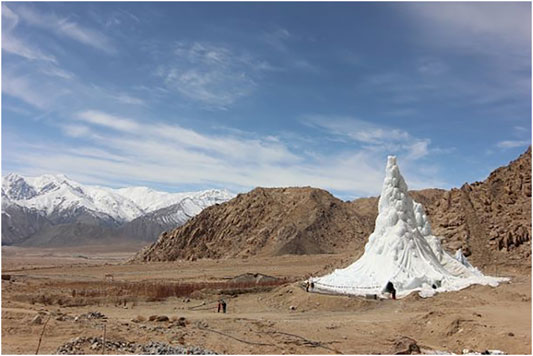
FIGURE 1. Icestupa in Ladakh, India on March 2017 was 24 m tall and contained around 3,700 m³ of water. Picture Credits: Lobzang Dadul.

However, to date, no reliable estimates exist about the quantity of meltwater an AIR can provide (Nüsser et al., 2019a). Moreover, preliminary estimates of AIRs in Ladakh indicate that they generate high water losses during their lifetimes (see Supplementary Appendix 7.1). During their accumulation period, AIRs can lose excessive fountain water and, during the ablation period, sublimation losses could also be significant. However, the relative contribution of these processes in the total water loss remains unknown.

In this paper, we develop a physically-based model of vertical AIRs (or Icestupas) that can estimate their freezing and melting rates. Mass and energy balance equations were used to estimate the quantity of ice, meltwater, sublimation and wastewater. Sensitivity and uncertainty analysis were performed to identify the most sensitive parameters and the variance they caused. For calibration, we chose two AIRs built across the winter of 2020/21 in India and Switzerland, and validated the model on a Swiss AIR built during winter 2019/20. Our model results provide a first step towards evaluating the potential of this decade old water storage technology worldwide (Wangchuk, 2014).

2 Study Sites and Data

The model requires three kinds of datasets containing weather, fountain and AIR volume measurements to accurately calibrate, estimate and validate the ice volume of AIRs. Through the winters of 2018/19, 2019/20 and 2020/21, such datasets were acquired for four AIRs in both Switzerland and India. Here, we present the results of three AIRs, which have a complete dataset. Two of them were constructed in the same Swiss location called Guttannen (referred to with the prefix CH) but during different winters, and the other was constructed at Gangles, India (referred to with the prefix IN). The 2020/21 AIR constructed on both these locations are shown in Figure 2.

FIGURE 2

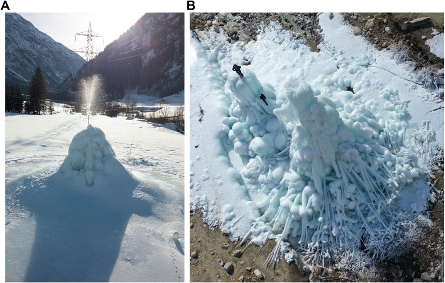
FIGURE 2. The Swiss and Indian AIRs were 5 m and 13 m tall on January 9 and March 3, 2021 respectively. Picture credits: Daniel Bürki (A) and Thinles Norboo (B).

The Guttannen site (46.66 °N, 8.29 °E) in the Bern region lies at 1047 m a.s.l.. In the winter (Oct-Apr), mean daily minimum and maximum air temperatures vary between -13 and 15 °C. Clear skies are rare, averaging around 7 days during winter. Daily winter precipitation can sometimes be as high as 100 mm. These values are based on 30 years of hourly weather model simulations (Meteoblue, 2021). The site was situated adjacent to a stream resulting in high humidity values across the study period as shown in Figure 2. AIR were constructed here by the Guttannen Bewegt Association during the winters of 2019–20 (CH20) and 2020–21 (CH21). Tree branches were laid covering the fountain pipe to initiate the ice formation process. The fountain height varied between 2 and 5 m during the construction period. The water was transferred from a spring water source and flowed via a flowmeter to the nozzle. In addition, a webcam guaranteed a continuous survey of the site during the construction of the AIR.

The Gangles site (34.22 °N, 77.61 °E) is located around 20 km north of Leh city in the Ladakh region, lying at 4025 m a.s.l.. The mean annual temperature is 5.6 °C, and the thermal range is characterized by high seasonal variation. During January, the coldest month, the mean temperature drops to − 7.2 °C. During August, the warmest month, the mean temperature rises to 17.5 °C (Nüsser et al., 2012). Because of the rain shadow effect of the Himalayan Range, the mean annual precipitation in Leh totals less than 100 mm, and there is high interannual variability. Whereas the average summer rainfall between July and September reaches 37.5 mm, the average winter precipitation between January and March amounts to 27.3 mm and falls almost entirely as snow. AIRs were constructed here as part of the Ice Stupa Competition by the Himalayan Institute of Alternatives, Ladakh (HIAL). The fountain height of the AIR varied between 5 and 9 m.

2.1 Meteorological Data

Air temperature, relative humidity, wind speed, pressure, longwave, shortwave direct and diffuse radiation are required to calculate the surface energy balance of an AIR (see Table 1). The study period starts when the fountain was first switched on and ends when the respective AIR melted completely. These two dates are denoted as start and expiry dates henceforth.

TABLE 1

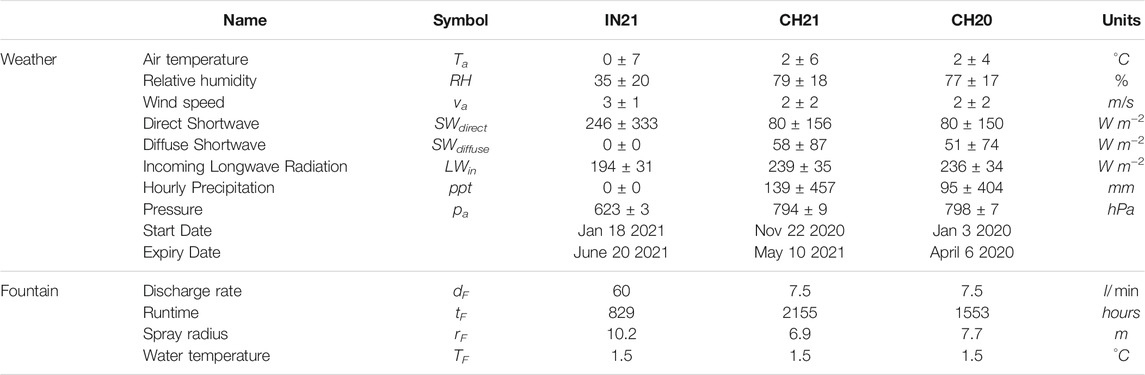
TABLE 1. Summary of the weather and fountain observations. The expiry date refers to the date when all of the ice of the AIR completely disappeared and only the dome volume remains. The weather measurements are shown using their mean (μ) and standard deviation (σ) during the study period as μ ± σ.

For the CH site, the primary weather data source was a meteoswiss AWS located 184 m away (Station ID: 0–756-0-GTT). In addition, we used ERA5 reanalysis dataset (Copernicus Climate Change Service (C3S), 2017) for filling data gaps and adding the shortwave and longwave radiation data that were not measured directly. The ERA5 reanalysis dataset is known to have a high correlation with sites in Switzerland (Scherrer, 2020). The Guttannen temperature dataset had a correlation greater than 0.8 with the ERA5 temperature for both winters. The ERA5 grid point chosen (46.64 °N, 8.25 °E) for the Swiss site was around 3.6 km away from the actual site. ERA5 variables (except incoming shortwave and longwave radiation) were fitted to the meteoswiss dataset via linear regressions. The zero wind speed values recorded by the meteoswiss AWS whenever snow accumulated on the ultrasonic wind sensor were replaced using the ERA5 dataset.

For the IN site, two different weather data sources were used to log all weather parameters required for the model. Temperature, humidity, wind speed and pressure data were logged with a weather station located 440 m away from the construction site. Shortwave radiation data were derived from another weather station located 15 km away. Unfortunately, precipitation was not logged. Since winter precipitation in Ladakh is less than 30 mm (Nüsser et al., 2012), we can safely assume negligible precipitation and mostly clear skies. As a consequence, the diffuse fraction of the global shortwave radiation was also assumed to be negligible. Temperature and humidity were measured with a rotronic sensor with an accuracy of ± 0.3 °C and ± 1% respectively. A young sensor measured the wind speed with an accuracy of ± 0.3 ms⁻¹ and a setra sensor measured the pressure with an accuracy of ± 0.01 hPa.

2.2 Fountain Observations

We define the fountain used through four attributes; namely, its spray radius, mean discharge rate, discharge runtime and water temperature as shown in Table 1. Continuous measurement of the discharge rate was unsuccessful in all sites due to data logger malfunctions of the associated flowmeter. Instead the discharge duration was first determined and then the available discharge measurement was used to determine the average discharge rate d_F during these periods. The spray radius r_F was estimated from the mean AIR circumference measured in the drone surveys during the fountain runtime.

The Swiss fountain discharge duration was extrapolated from just one fountain on and off event each. Even though the Indian fountain was never manually switched off, there were many pipeline freezing events that interrupted the discharge duration. Discharge rate was extrapolated to be the mean discharge rate d_F except during these pipeline freezing events.

2.3 Drone Surveys

Several photogrammetric surveys using drones were conducted on the Swiss and Indian sites. The details of these surveys and the methodology used to produce the corresponding outputs are explained in Supplementary Appendix 7.2. The digital elevation maps (DEMs) generated from the obtained imagery were analysed to document the radius, surface area and volume of the ice structure. The number of surveys conducted for the IN21, CH21 and CH20 AIRs were six, eight and two, respectively (see Table 2). The first drone flight was used to set the dome volume (V_dome) for model initialisation. The remaining surveys were used for model calibration and validation. Since the Indian AIR was built on top of another ice structure (see Figure 2), it had a much higher dome volume compared to the other AIRs.

TABLE 2

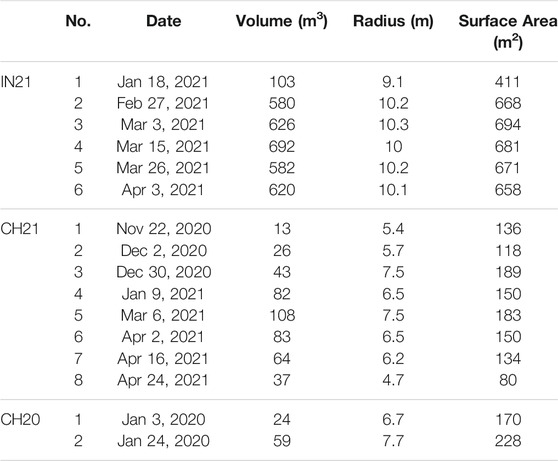
TABLE 2. Summary of the drone surveys.

3 Model Setup

A bulk energy and mass balance model is used to calculate the amounts of ice, meltwater, water vapour and wastewater of the AIR. In each hourly time step, the model uses the AIR surface area, energy balance and mass balance calculations to estimate its ice volume, surface temperature and wastewater as shown in Figure 3 .

FIGURE 3

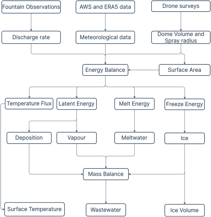
FIGURE 3. Model schematic showing the workflow used in the model at every time step.

3.1 Surface Area Calculation

The model assumes the AIR shape to be a cone and assigns the following shape attributes:

$\begin{array}{ll}\hfill A_{cone}^i& =\pi \cdot r_{cone}^i\cdot \sqrt{{(r_{cone}^i)}^2+{(h_{cone}^i)}^2}\hfill \end{array}(\mathrm{1a})$

$\begin{array}{ll}\hfill V_{cone}^i& =\pi /3\cdot {(r_{cone}^i)}^2\cdot h_{cone}^i\hfill \end{array}(\mathrm{1b})$

$\begin{array}{ll}\hfill j_{cone}^i& =\frac{\mathrm{\Delta }{M}_{ice}^i}{{\rho }_{water}\ast A_{cone}^i}\hfill \end{array}(\mathrm{1c})$

where i denotes the model time step, $r_{cone}^i$ is the radius; $h_{cone}^i$ is the height; $A_{cone}^i$ is the surface area; $V_{cone}^i$ is the volume and $j_{cone}^i$ is the AIR surface normal thickness change as shown in Figure 4. $M_{ice}^i$ is the mass of the AIR and $\mathrm{\Delta }{M}_{ice}^i=M_{ice}^{i-1}-M_{ice}^{i-2}$. Henceforth, the equations used display the model time step superscript i only if it is different from the current time step.

FIGURE 4

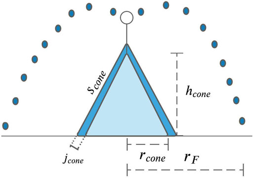
FIGURE 4. Shape variables of the AIR. r_cone is the radius, h_cone is the height, j_cone is the thickness change and s_cone is the slope of the ice cone. r_F is the spray radius of the fountain.

AIR volume can also be expressed as:

$V_{cone}=\frac{M_{ice}}{{\rho }_{ice}}(2)$

where ρ_ice is the density of ice (917 kg m⁻³).

The initial radius of the AIR is assumed to be r_F. The initial height h₀ depends on the dome volume V_dome used to construct the AIR as follows:

$h_0=\mathrm{\Delta }x+\frac{3\cdot V_{dome}}{\pi \cdot {(r_F)}^2}(3)$

where Δx is the surface layer thickness (defined in Section 3.2)

During the subsequent time steps, the dimensions of the AIR evolve assuming a uniform thickness change (j_cone) across its surface area with an invariant slope $s_{cone}=\frac{h_{cone}}{r_{cone}}$ . During these time steps, the volume is parameterised using Eq. 1b as:

$V_{cone}=\frac{\pi \cdot {(r_{cone})}^3\cdot s_{cone}}{3}(4)$

We define the Icestupa boundary through its spray radius, i.e. we assume ice formation is negligible when r_cone > r_F. Combining Eqs 1b, 2 Eqs 3, 4, 4, the geometric evolution of the Icestupa at each time step i can be determined by considering the following rules:

$(r_{cone},h_{cone})=\left\{\begin{array}{cc}(r_F,h_0)\hfill & ifi=0\hfill \\ \left(r_{cone}^{i-1},\frac{3\cdot M_{ice}}{\pi \cdot {\rho }_{ice}\cdot {(r_{cone}^{i-1})}^2}\right)\hfill & if{r}_{cone}^{i-1}\ge r_F\mathit{\text{and}}\mathrm{\Delta }{M}_{ice}>0\hfill \\ {\left(\frac{3\cdot M_{ice}}{\pi \cdot {\rho }_{ice}\cdot s_{cone}}\right)}^{1/3}\cdot (1,s_{cone})\hfill & otherwise\hfill \end{array}\right.(5)$

3.2 Energy Balance Calculation

We approximate the energy balance at the surface of an AIR by a one-dimensional description of energy fluxes into and out of a (thin) layer with thickness Δx:

${\rho }_{ice}\cdot c_{ice}\cdot \frac{\mathrm{\Delta }T}{\mathrm{\Delta }t}\cdot \mathrm{\Delta }x=q_{SW}+q_{LW}+q_L+q_S+q_F+q_G(6)$

Upward and downward fluxes relative to the ice surface are positive and negative, respectively. The first term is the energy change of the surface layer, which can be translated into a phase change energy should phase changes occur; q_SW is the net shortwave radiation; q_LW is the net longwave radiation; q_L and q_S are the turbulent latent and sensible heat fluxes. q_F represents the heat exchange of the fountain water droplets with the AIR ice surface. q_G represents ground heat flux between the AIR surface and its interior.

The energy flux acts upon the AIR surface layer, which has an upper and lower boundary defined by the atmosphere and the ice body of the AIR, respectively. A sensitivity analysis was later performed to understand the influence of this factor and decide its value. Here, we define the surface temperature T_ice to be the modelled average temperature of the icestupa surface layer.

3.2.1 Net Shortwave Radiation q_SW

The net shortwave radiation q_SW is computed as follows:

$q_{SW}=(1-\alpha )\cdot (S{W}_{direct}\cdot f_{cone}+S{W}_{diffuse})(7)$

where SW_direct and SW_diffuse are the direct and diffuse shortwave radiation, α is the modelled albedo and f_cone is the area fraction of the ice structure exposed to the direct shortwave radiation.

The albedo varies depending on the water source that formed the current AIR surface layer. During the fountain runtime, the albedo assumes a constant value corresponding to ice albedo. However, after the fountain is switched off, the albedo can reset to snow albedo during snowfall events and then decay back to ice albedo. We use the scheme described in Oerlemans and Knap (1998) to model this process. The scheme records the decay of albedo with time after fresh snow is deposited on the surface. δt records the number of time steps after the last snowfall event. After snowfall, albedo changes over a time step, δt , as

$\alpha ={\alpha }_{ice}+({\alpha }_{snow}-{\alpha }_{ice})\cdot e^{(-\delta t)/\tau }(8)$

where α_ice is the bare ice albedo value (0.25), α_snow is the fresh snow albedo value (0.85) and τ is a decay rate (16 days), which determines how fast the albedo of the ageing snow recedes back to ice albedo.

The solar area fraction f_cone of the ice structure exposed to the direct shortwave radiation depends on the shape considered. Using the solar elevation angle θ_sun, the solar beam can be considered to have a vertical component, impinging on the horizontal surface (semicircular base of the AIR), and a horizontal component impinging on the vertical cross section (a triangle). The solar elevation angle θ_sun used is modelled using the parametrisation proposed by Woolf (1968). Accordingly, f_cone is determined as follows:

$f_{cone}=\frac{(0.5\cdot r_{cone}\cdot h_{cone})\cdot \mathit{cos}{\theta }_{sun}+(\pi \cdot {(r_{cone})}^2/2)\cdot \mathit{sin}{\theta }_{sun}}{\pi \cdot r_{cone}\cdot {({(r_{cone})}^2+{(h_{cone})}^2)}^{1/2}}(9)$

The diffuse shortwave radiation is assumed to impact the conical AIR surface uniformly.

3.2.2 Net Longwave Radiation q_LW

The net longwave radiation q_LW is determined as follows:

$q_{LW}=L{W}_{in}-\sigma \cdot {ϵ}_{ice}\cdot {(T_{ice}+273.15)}^4(10)$

where T_ice is the modelled surface temperature given in [°C], σ = 5.67 ⋅ 10⁻⁸ Jm⁻²s⁻¹K⁻⁴ is the Stefan-Boltzmann constant, LW_in denotes the incoming longwave radiation and ϵ_ice is the corresponding emissivity value for the Icestupa surface (0.97).

The incoming longwave radiation LW_in for the Indian site, where no direct measurements were available, is determined as follows:

$L{W}_{in}=\sigma \cdot {ϵ}_a\cdot {(T_a+273.15)}^4(11)$

here T_a represents the measured air temperature and ϵ_a denotes the atmospheric emissivity. We approximate the atmospheric emissivity ϵ_a using the equation suggested by Brutsaert (1982), considering air temperature and vapor pressure (Eqn. 12). The vapor pressure of air over water and ice was obtained using Eq. (15). The expression defined in Brutsaert (1975) for clear skies (first term in equation 12) is extended with the correction for cloudy skies after Brutsaert (1982) as follows:

${ϵ}_a=1.24\cdot {\left(\frac{p_{v,w}}{(T_a+273.15)}\right)}^{1/7}\cdot (1+0.22\cdot {cld}^2)(12)$

with a cloudiness index cld, ranging from 0 for clear skies to 1 for complete overcast skies. For the Indian site, we assume cloudiness to be negligible.

3.2.3 Turbulent Fluxes

The turbulent sensible q_S and latent heat q_L fluxes are computed with the following expressions proposed by Garratt (1992):

$q_S={\mu }_{cone}\cdot c_a\cdot {\rho }_a\cdot p_a/p_{0,a}\cdot \frac{{\kappa }^2\cdot v_a\cdot (T_a-T_{ice})}{{\left(\ln \frac{h_{AWS}}{z_0}\right)}^2}(13)$

$q_L={\mu }_{cone}\cdot 0.623\cdot L_s\cdot {\rho }_a/p_{0,a}\cdot \frac{{\kappa }^2\cdot v_a(p_{v,w}-p_{v,ice})}{{\left(\ln \frac{h_{AWS}}{z_0}\right)}^2}(14)$

where h_AWS is the measurement height above the ground surface of the AWS (around 2 m for all sites), v_a is the wind speed in [m s⁻¹], c_a is the specific heat of air at constant pressure (1010 J kg⁻¹K⁻¹), ρ_a is the air density at standard sea level (1.29 kgm⁻³), p_0,a is the air pressure at standard sea level (1013 hPa), p_a is the measured air pressure, κ is the von Karman constant (0.4), z₀ is the surface roughness (3 mm) and L_s is the heat of sublimation (2848 kJ kg⁻¹). The vapor pressure of air with respect to water (p_v,w) and with respect to ice (p_v,ice) was obtained using the formulation given in Huang (2018) :

$\begin{array}{cc}\hfill p_{v,w}& =e^{\frac{\left(34.494-\frac{4924.99}{T_a+237.1}\right)}{{(T_a+105)}^{1.57}\cdot 100}}\cdot \frac{RH}{100}\hfill \\ \hfill p_{v,ice}& =e^{\frac{\left(43.494-\frac{6545.89}{T_{ice}+278}\right)}{{(T_{ice}+868)}^2\cdot 100}}\hfill \end{array}(15)$

The dimensionless parameter μ_cone is an exposure parameter that deals with the fact that AIR has a rough appearance and forms an obstacle to the wind regime. This factor accounts for the larger turbulent fluxes due to the roughness of the surface (Oerlemans et al., 2021), and is a function of the AIR slope as follows:

${\mu }_{cone}=1+\frac{s_{cone}}{2}(16)$

A possible source of error is the fact that wind measurements from the horizontal plane at the AWS are used, which might be different from those on a slope. However, without detailed datasets from the AIR surface, we retain this assumption.

3.2.4 Fountain Discharge Heat Flux q_F

The fountain water, at temperature T_F, is assumed to cool to 0 °C. Thus, the heat flux caused by this process is:

$q_F=\frac{\mathrm{\Delta }{M}_F\cdot c_{water}\cdot T_F}{\mathrm{\Delta }t\cdot A_{cone}}(17)$

with c_water as the specific heat of water (4186 J kg⁻¹K⁻¹).

3.2.5 Bulk Icestupa Heat Flux q_G

The bulk Icestupa heat flux q_G corresponds to the ground heat flux in normal soils and is caused by the temperature gradient between the surface layer (T_ice) and the ice body (T_bulk). It is expressed by using the heat conduction equation as follows:

$q_G=k_{ice}\cdot (T_{bulk}-T_{ice}^{i-1})/l_{cone}(18)$

where k_ice is the thermal conductivity of ice (2.123 W m⁻¹ K⁻¹) , T_bulk is the mean temperature of the ice body within the icestupa and l_cone is the average distance of any point in the surface to any other point in the ice body. T_bulk is initialised as 0 °C and later determined from Eq. 18 as follows:

$T_{bulk}^{i+1}=T_{bulk}-(q_G\cdot A\cdot \mathrm{\Delta }t)/(M_{ice}\cdot c_{ice})(19)$

Since AIRs typically have conical shapes with r_cone > h_cone, we assume that the center of mass of the cone body is near the base of the fountain. Thus, the distance of every point in the AIR surface layer from the cone body’s center of mass is between h_cone and r_cone. Therefore, we calculate q_G assuming l_cone = (r_cone + h_cone)/2.

3.2.6 Phase Changes

In this section, the numerical procedures to model phase changes at the surface layer are explained. Let T_temp be the calculated surface temperature. Therefore, Eq. (6) can be rewritten as:

$q_{total}={\rho }_{ice}\cdot c_{ice}\cdot \frac{(T_{temp}-T_{ice})}{\mathrm{\Delta }t}\cdot \mathrm{\Delta }x$

where q_total represents the total energy available to be redistributed. Even if the numerical heat transfer solution produces temperatures which are T_temp > 0°C, say from intense shortwave radiation, the ice temperature must remain at T_temp = 0°C. The “excess” energy is used to drive the melting process. Moreover, the energy input is used to melt the surface ice layer, and not to raise the surface temperature to some unphysical value. Similarly, for freezing to occur, three conditions are required. Firstly, fountain water is present (ΔM_F > 0) and secondly the calculated temperature of the ice, T_temp, is below 0°C. However, these two conditions are not sufficient as the latent heat turbulent fluxes can only contribute to temperature fluctuations. Therefore, an additional condition, namely, (q_total − q_L) < 0, is required. Depending on the above conditions, the total energy q_total can be redistributed for the melting (q_melt), freezing (q_freeze) and surface temperature change (q_T) processes as follows:

$q_{total}=\left\{\begin{array}{cc}{q}_{freeze}+q_T\hfill & if\mathrm{\Delta }{M}_F>0\mathit{\text{and}}{T}_{temp}<0\mathit{\text{and}}(q_{total}-q_L)<0\hfill \\ q_{melt}+q_T\hfill & \mathit{\text{otherwise}}\hfill \end{array}\right.(20)$

Henceforth, time steps when the total energy is redistributed to the freezing energy are called freezing events and the rest of the time steps are called melting events.

During a freezing event, the AIR surface is assumed to warm to 0°C. The available energy (q_total − q_L) is further increased due to this change in surface temperature represented by the energy flux:

$q_0=\frac{{\rho }_{ice}\cdot \mathrm{\Delta }x\cdot c_{ice}\cdot T_{ice}^{i-1}}{\mathrm{\Delta }t}$

The available fountain discharge (ΔM_F) may not be sufficient to utilize all the freezing energy. At such times, the additional freezing energy further cools down the surface temperature. Accordingly, the surface energy flux distribution during a freezing event can be represented as:

$(q_{freeze},q_T)=\left\{\begin{array}{cc}\left(\frac{\mathrm{\Delta }{M}_F\cdot L_f}{A_{cone}\cdot \mathrm{\Delta }t},q_{total}+\frac{\mathrm{\Delta }{M}_F\cdot L_f}{A_{cone}\cdot \mathrm{\Delta }t}\right)\hfill & if\mathrm{\Delta }{M}_{F}insufficient\hfill \\ (q_{total}-q_L+q_0,q_L-q_0)\hfill & \mathit{\text{otherwise}}\hfill \end{array}\right.(21)$

If T_temp > 0°C, then energy is reallocated from q_T to q_melt to maintain surface temperature at melting point. The total energy flux distribution during a melting event can be represented as:

$(q_{melt},q_T)=\left\{\begin{array}{cc}(0,q_{total})\hfill & if{T}_{temp}\le 0\hfill \\ \left(\frac{T_{temp}\cdot {\rho }_{ice}\cdot c_{ice}\cdot \mathrm{\Delta }x}{\mathrm{\Delta }t},q_{total}-\frac{T_{temp}\cdot {\rho }_{ice}\cdot c_{ice}\cdot \mathrm{\Delta }x}{\mathrm{\Delta }t}\right)\hfill & if{T}_{temp}>0\hfill \end{array}\right.(22)$

3.3 Mass Balance Calculation

The mass balance equation for an AIR is represented as:

$\frac{\mathrm{\Delta }{M}_F+\mathrm{\Delta }{M}_{ppt}+\mathrm{\Delta }{M}_{dep}}{\mathrm{\Delta }t}=\frac{\mathrm{\Delta }{M}_{ice}+\mathrm{\Delta }{M}_{water}+\mathrm{\Delta }{M}_{sub}+\mathrm{\Delta }{M}_{waste}}{\mathrm{\Delta }t}(23)$

where M_F is the cumulative mass of the fountain discharge; M_ppt is the cumulative precipitation; M_dep is the cumulative accumulation through water vapour deposition; M_ice is the cumulative mass of ice; M_water is the cumulative mass of melt water; M_sub represents the cumulative water vapor loss by sublimation and M_waste represents the fountain wastewater that did not interact with the AIR. The left hand side of Eq. 23 represents the rate of mass input and the right hand side represents the rate of mass output for an AIR.

Precipitation input is calculated as shown in Eq. 24b where ρ_w is the density of water (1000 kg m⁻³), Δppt/Δt is the measured precipitation rate in [m s⁻¹] and T_ppt is the temperature threshold below which precipitation falls as snow. Here, snowfall events were identified using T_ppt as 1°C. Snow mass input is calculated by assuming a uniform deposition over the entire circular footprint of the AIR.

The latent heat flux is used to estimate either the evaporation and condensation processes or sublimation and deposition processes as shown in Equation (24c). During the time steps at which the surface temperature is below 0 °C only sublimation and deposition can occur, but if the surface temperature reaches 0 °C, evaporation and condensation can also occur. As the differentiation between evaporation and sublimation (and condensation and deposition) when the air temperature reaches 0 °C is challenging, we assume that negative (positive) latent heat fluxes correspond only to sublimation (deposition), i.e. no evaporation (condensation) is calculated.

Since we have categorized every time step as a freezing or melting event, we can determine the melting/freezing rates and the corresponding meltwater/ice quantities as shown in Eqs 24e, 24d, and 24f. Having calculated all other mass components, the fountain wastewater generated every time step can be calculated using Eq. 23.

$\begin{array}{ll}\hfill \frac{\mathrm{\Delta }{M}_F}{\mathrm{\Delta }t}=& \left\{\begin{array}{cc}\frac{60}{{\rho }_w\cdot \mathrm{\Delta }t}\cdot d_F\hfill & iffountain\mathit{\text{is on}}\hfill \\ 0\hfill & \mathit{\text{otherwise}}\hfill \end{array}\right.\hfill \end{array}(\mathrm{24a})$

$\begin{array}{ll}\hfill \frac{\mathrm{\Delta }{M}_{ppt}}{\mathrm{\Delta }t}=& \left\{\begin{array}{cc}\pi \cdot {(r_{cone})}^2\cdot {\rho }_w\cdot \frac{\mathrm{\Delta }ppt}{\mathrm{\Delta }t}\hfill & if{T}_a<T_{ppt}\hfill \\ 0\hfill & if{T}_a\ge T_{ppt}\hfill \end{array}\right.\hfill \end{array}(\mathrm{24b})$

$\begin{array}{ll}\hfill \left(\frac{\mathrm{\Delta }{M}_{dep}}{\mathrm{\Delta }t},\frac{\mathrm{\Delta }{M}_{sub}}{\mathrm{\Delta }t}\right)=& \left\{\begin{array}{cc}\frac{q_L\cdot A_{cone}}{L_s}\cdot (\mathrm{1,0})\hfill & if{q}_L\ge 0\hfill \\ \frac{q_L\cdot A_{cone}}{L_s}\cdot (0,-1)\hfill & if{q}_L<0\hfill \end{array}\right.\hfill \end{array}(\mathrm{24c})$

$\begin{array}{ll}\hfill \frac{\mathrm{\Delta }{M}_{water}}{\mathrm{\Delta }t}=& \frac{q_{melt}\cdot A_{cone}}{L_f}\hfill \end{array}(\mathrm{24d})$

$\begin{array}{ll}\hfill \frac{\mathrm{\Delta }{M}_{freeze/melt}}{\mathrm{\Delta }t}=& \frac{q_{freeze/melt}\cdot A_{cone}}{L_f}\hfill \end{array}(24e)$

$\begin{array}{ll}\hfill \frac{\mathrm{\Delta }{M}_{ice}}{\mathrm{\Delta }t}=& \frac{q_{freeze}\cdot A_{cone}}{L_f}+\frac{\mathrm{\Delta }{M}_{ppt}}{\mathrm{\Delta }t}+\frac{\mathrm{\Delta }{M}_{dep}}{\mathrm{\Delta }t}-\frac{\mathrm{\Delta }{M}_{sub}}{\mathrm{\Delta }t}-\frac{\mathrm{\Delta }{M}_{water}}{\mathrm{\Delta }t}\hfill \end{array}(\mathrm{24f})$

Considering AIRs as water reservoirs, their net water loss can be defined as:

$\mathit{\text{Net water losses}}=\frac{M_{waste}+M_{sub}}{(M_F+M_{ppt}+M_{dep})}\cdot 100(25)$

3.4 Uncertainty Quantification

The uncertainty in the model of estimating ice volumes is caused by three sources, namely, model forcing data, model hyperparameters and model parameters. Model forcing data can further be divided into weather and fountain forcing data. Significant uncertainty exists in the weather forcing data, particularly for all the radiation measurements (SW_direct, SW_diffuse, LW_in) since they were taken from ERA5 dataset or an AWS far away from the construction sites. Since no other weather datasets exist for comparison, especially near the IN21 AIR, we are not accounting for uncertainties related to meteorological forcing data in this analysis. Uncertainty in the fountain forcing data arises due to only some fountain parameters listed in Table 3. Fountain runtime t_F has no uncertainty for the Swiss AIRs because no interruptions occured during the study period. However, significant uncertainty exists for the IN21 AIR , where the interruptions due to pipeline freezing events happened overnight but this was ignored in this analysis. Fountain spray radius r_F was measured using the drone survey and therefore also doesn’t contribute to model uncertainty. The choice of mean discharge rate d_F for both sites was just a best guess, based on few observations made by the flowmeter. So we associate this parameter by a large uncertainty of ± 50 %. For the fountain water temperature T_F, we assumed an upper bound of 3 °C since it is unlikely for it to have been beyond this range considering winter conditions at all the sites. The model structure introduces uncertainty through the spatial and temporal hyperparameters Δx and Δt. By definition, Δx is directly proportional to Δt. Therefore, we fix the temporal resolution of the model at hourly timesteps and only investigate the uncertainty caused by Δx here. Since the surface layer thickness for an AIR does not resemble to any parameter in the glaciological literature, we attribute a wide range of values for it (from 1 to 10 cm). The model parameters are henceforth called as weather parameters to distinguish them from the fountain forcing parameters. These were fixed within a range based on literature values (see Table 3).

TABLE 3

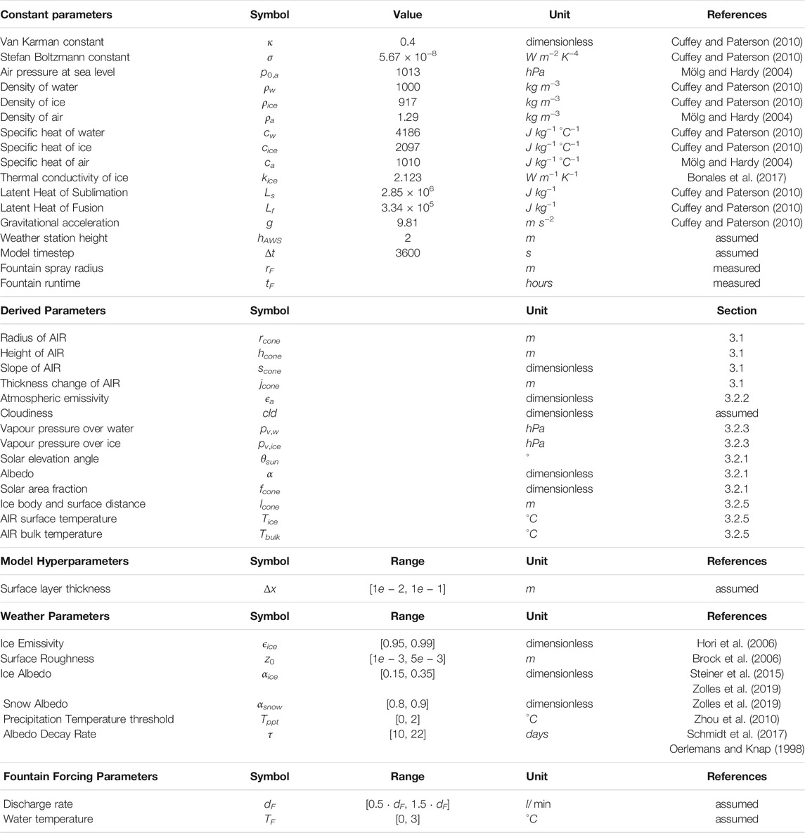
TABLE 3. Free parameters in the model categorised as constant, derived, model hyperparameters, weather and fountain forcing parameters with their respective values/ranges.

The three types of uncertain parameters namely, model hyperparameters (Δx), fountain forcing parameters (d_F, T_F) and weather parameters (ϵ_ice, z₀, α_ice, α_snow, T_ppt, τ) are denoted as Q^M, Q^F and Q^W henceforth. Together, these nine parameters cause a large uncertainty in the ice volume estimates. In order to reduce this uncertainty, we perform a global sensitivity analysis with the net water loss as our objective. The objective of this sensitivity analysis was to reduce the dimension of the parameter space by calibrating the parameters with high total-order sensitivities ($S_{T_j}>0.5$). The methodology to determine $S_{T_j}$ is described in Supplementary Appendix 7.3. These sensitive model parameters were calibrated based on the root mean squared error (RMSE) between the drone surveys (see Table 2) and the model estimations of the ice volume. For this calibration procedure, all the other parameters were set to the median value of their respective ranges defined in Table 3. The sensitivity analysis and calibration were carried out with the drone surveys of CH21 and IN21 AIRs.

The model uncertainty was quantified separately for the remaining parameters in Q^M, Q^F and Q^W using the corresponding 90 % prediction interval I^M, I^F and I^W. The 90 % prediction interval, I^k, gives us the interval within which 90 % of the ice volume outcomes occur when all the parameters in Q^k are varied assuming each has an independent uniform probability density function. 5 % of the outcomes are above and 5 % are below this interval. The methodology to obtain this is described in Supplementary Appendix 7.3.

For validation, the calibrated model was tested with two datasets namely, the expiry date of all AIRs and the drone surveys of CH20 AIR.

4 Results

4.1 Calibration of Sensitive Parameters

The total-order sensitivities of all the nine parameters with respect to the net water loss objective are shown in Figure 5A . In total, the global sensitivity analysis required 1432 model runs to determine these sensitivities for each site. The only sensitive parameter ($S_{T_j}>0.5$) for both AIRs was the surface layer thickness. The RMSE between the drone surveys and the model ice volume estimates for different surface layer thickness are shown in Figure 5B. The optimum value of Δx was found to be 45 and 65 mm with an RMSE of 9 m³ and 30 m³ for CH21 and IN21 AIRs respectively.

FIGURE 5

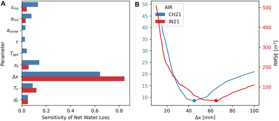
FIGURE 5. (A) Total-order sensitivities of all the uncertain parameters of the model with net water loss as the objective. (B) The calibration of the sensitive parameter, Δx with the RMSE between the drone and model estimates of the ice volume. The dots denote the optimum values. The estimates from the Swiss and Indian AIRs are denoted with blue and red colors respectively.

4.2 Weather and Fountain Forcing Uncertainty Quantification

The uncertainty in the ice volume estimates caused by the weather and fountain forcing parameters are shown in Figure 6. The ranges highlighted represent the corresponding 90 % prediction interval of the ice volume estimates. Weather uncertainty determination required 422 simulations whereas fountain forcing uncertainty determination required 32 simulations for each AIR. Since the results presented below differ significantly during the fountain runtime, we divided the simulation duration of the AIR into accumulation and ablation periods. The accumulation (ablation) period ends (starts) at the last fountain discharge event.

FIGURE 6

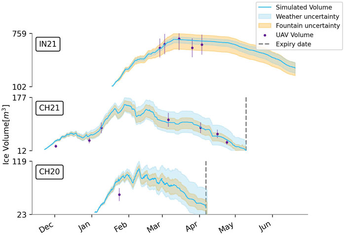
FIGURE 6. Simulated ice volume during the lifetime of the AIRs (blue curve). The shaded regions (light blue and orange) represent the 90% prediction interval of the AIR ice volume caused by the variations in weather and fountain forcing parameters, respectively. Violet points indicate the drone ice volume observations. The grey dashed line represents the observed expiry date for each AIR.

The prediction interval of the weather and fountain forcing parameters behave differently during the accumulation and ablation period for all AIRs. Prediction interval of the weather parameters increase throughout the simulation period, but that of the fountain forcing parameters only increase during the accumulation period. This is to be expected since the fountain forcing parameters directly affect the model estimates only during the accumulation period.

Weather uncertainty for the Indian site was low compared to the Swiss since precipitation and the associated variation in albedo was negligible. At the end of the accumulation period, the Indian weather prediction interval had a magnitude of 73 m³ which was 10 % of the maximum simulated volume, whereas the magnitude of the Swiss weather prediction interval was much higher (28 % of the maximum simulated volume for the CH21 AIR). This was expected since four out of the six uncertain Indian weather parameters were part of the albedo module. Among all the weather parameters, surface roughness caused the most variance in both Indian and the Swiss ice volume estimates.

Fountain forcing uncertainty for the Indian site was higher than its weather uncertainty (28 % of the maximum simulated volume at the end of the accumulation period). This was predominantly due to the uncertainty in the fountain’s water temperature. However, for the Swiss site, the prediction interval of the fountain forcing parameters was similar to that of the weather parameters during the accumulation period. Since the mean fountain discharge rate of the Indian location was eight times that of the Swiss, the uncertainty due to the fountain forcing parameters was expected to be larger for the Indian location.

4.3 Validation

Model performance can be judged based on the ice volume left on the expiry date of all AIRs. In the case of CH21 AIR no ice volume was left whereas for CH20 AIR ice volume of 12 m³ was left on the expiry date. For the IN21 AIR, the determination of the expiry date was not possible. In reality, the IN21 AIR was found to have disintegrated into several ice blocks on 20th June 2021.

There was also one drone survey of the CH20 AIR volume for validation purposes (see Table 2). The RMSE of that observation with the modelled volume was 19 m³ which is 18 % of the maximum simulated ice volume of CH20 AIR.

4.4 AIR Ice Volume Estimates

Since this model used a surface energy balance model commonly applied on glaciers, we analyse the AIR temporal and spatial variation similar to how it is done for a glacier. Particularly, we used the AIR surface normal thickness change (j_cone) as a measure to quantify the location influence. Note that j_cone is similar to the “specific mass balance” of a glacier with units m w. e. The thickness change during the accumulation and ablation period was referred to as thickness growth and decay, respectively.

The construction decisions responsible for the observed magnitude and variance of the ice volume estimates can be categorised based on the fountain used and the location selected. According to Eq. 24e, the freezing/melting rate of the AIRs can be decomposed to the corresponding freezing/melting energy and the surface area. The construction location chosen determines the thickness growth/decay through the freezing/melting energy flux and the fountain determines the surface area through its spray radius.

The influence of location can be further comprehended if we analyse the daily surface normal thickness change together with the corresponding energy fluxes. Figure 7 shows the daily thickness and energy balance components calculated with the calibrated surface layer thickness for the first and last 20 days for each AIR. The two time periods selected were characteristic of the accumulation and ablation period, respectively. A strong variability was evident between the accumulation and ablation periods and between the CH21 and the IN21 AIRs.

FIGURE 7

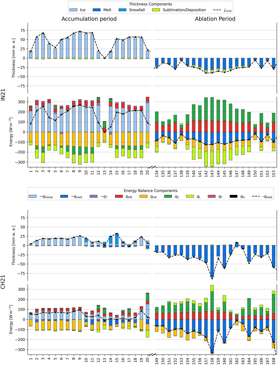
FIGURE 7. Daily averages of thickness and energy balance components for the Indian and Swiss AIRs during the first 20 days of the accumulation and the last 20 days of the ablation period respectively.

The daily mean thickness change of the Indian location was positive (3 mm w.e.) with a daily mean growth of 31 mm w.e. and a mean decay of 11 mm w.e. In the Swiss location, the daily mean thickness change was negative ( − 4 mm w.e.) with a daily mean thickness growth of 8 mm w.e. and a mean decay of 18 mm w.e. The difference in magnitude between the growth and the decay corresponds to the difference between the freezing and the melting energy balance components. For the Indian site, q_freeze accounted for 73 %, q_melt accounted for 23 % and q_T just 4 % of overall energy turnover. The energy turnover is calculated as the sum of energy fluxes in absolute values. For the Swiss site, q_freeze accounted for 37 %, q_melt accounted for 61 % and q_T just 2 % of overall energy turnover. The freezing events occurred for 19 and 34% of the simulation duration (see Table 1) for the Indian and Swiss sites, respectively. The accumulation period is characteristic of these freezing events and the ablation period is characteristic of the melting events. We compare the energy turnover of different energy fluxes between these two periods to quantify the influence of different surface processes.

To understand the overall impact of the radiation fluxes (longwave and shortwave) and the turbulent fluxes (sensible and latent) on the freezing and melting energies, we sum their respective energy turnover by taking into account the sign of their mean energy during the accumulation/ablation period (see Table 4). A negative sign indicates that the corresponding energy flux increased/decreased the freezing/melting energy respectively. Note that all energy fluxes maintain the same sign for both accumulation and ablation periods for the Indian location, but the latent heat changes sign for the Swiss location. The radiation fluxes contributed -27 and 0 % to the freezing and melting energies for the Indian location and -20 % and -6 % to the Swiss location, respectively. Similarly, the turbulent fluxes at the Indian location contribute -11 and 10 % and at the Swiss location contribute 12 and 49% respectively. Therefore, the AIR thickness growth was driven by the net radiation fluxes and the AIR thickness decay was driven by the net turbulent fluxes.

TABLE 4

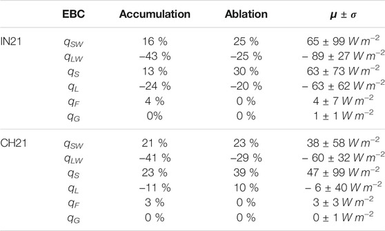
TABLE 4. Contribution of the energy balance components (EBC) to the total energy turnover (the sum of energy fluxes in absolute values) during the accumulation and ablation periods with their daily mean (μ) and standard deviation (σ) for each site. The positive/negative sign is indicative of the upward/downward direction of the mean energy flux during the respective period.

The longwave radiation flux had the highest energy turnover during the accumulation period for both locations. It increased and decreased the freezing and melting energy balance components during the accumulation and ablation period, respectively. However, its magnitude was much lower in the ablation period compared to the accumulation period since the rising air temperature increased the incoming longwave radiation in the ablation period. The mean longwave radiation flux (see Table 4) was lower for the Indian site as its incoming longwave radiation was strongly reduced due to cloud free skies. (see Table 1).

Global shortwave radiation was around two times higher for the Indian location due to its higher altitude and lower latitude. However, the energy turnover of the shortwave radiation for both sites were similar (see Table 4). The main cause of this is the differential exposure of a conical structure to direct and diffuse fractions of global shortwave radiation. This effect is quantified by the area fraction parameter f_cone. Less than 20 % of the AIR surface area on average was exposed to direct shortwave radiation flux for both locations. Cloudy days increase the diffuse fraction of global shortwave radiation. Therefore, the net shortwave radiation impact for the Indian site was significantly reduced as the study period had mostly clear days. Since the Swiss site had many cloudy days, its higher diffuse shortwave radiation enhanced the net shortwave radiation impact (see Table 1). Temporal variation in the f_cone factor due to increasing solar elevation angle and decreasing AIR slope leads to higher shortwave radiation in the ablation period compared to the accumulation period. Albedo, on the other hand, only varied temporally for the Swiss location because there was no precipitation for the Indian site.

Turbulent fluxes play an essential role in the energy balance. Sensible heat fluxes had the highest energy turnover during the ablation period for both locations. It decreased and increased the freezing and melting energy balance components respectively. The Indian location had a much higher sensible heat due to higher wind speeds and higher temperature gradient between the AIR surface and the atmosphere. The sensible heat contributes much more to the energy turnover during ablation period than the latent heat flux due to rising air temperature. Alternatively, latent heat flux does not vary much in energy turnover between the accumulation and ablation periods. For the Indian site, latent heat flux increased and decreased the freezing and melting energy, since sublimation was favoured throughout the simulation duration. On the contrary, for the Swiss location, latent heat increased both the freezing and the melting energy, as sublimation and deposition were favoured during the accumulation and ablation periods, respectively.

The mass contribution of the sublimation/deposition process (shown in Table 5) was significantly smaller than the energy flux contribution of this process (shown in Table 4), since the heat of vaporization is around nine times higher than the heat of fusion. The magnitude of the sublimation/deposition process was significantly different for both AIRs: IN21 AIR lost 2 % of its mass input to sublimation compared to the 1 % mass loss of CH21 AIR (see Table 5). For the IN21 AIR, the mass gain due to deposition was an order of magnitude smaller than the mass loss due to sublimation. For the CH21 AIR, there were no significant differences between the mass lost by sublimation and the mass gained by deposition. This was expected, since glaciers near the IN21 location have been hypothesized to lose a significant amount of their mass through sublimation, as suggested by Azam et al. (2018).

TABLE 5

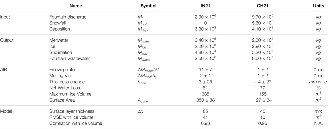
TABLE 5. Summary of the mass balance and AIR characteristics estimated at the end of the respective simulation duration.

The fountain had some influence on the energy fluxes through its water temperature, temperature forcing and albedo forcing. However, this influence was insignificant compared to its influence on the surface area which was directly proportional to the fountain’s spray radius during the accumulation period. Therefore, the thickness growth was uniformly scaled to produce the corresponding ice volume. Additionally, the higher spray radius of the Indian fountain resulted in a higher maximum ice volume. Nonetheless, this was accompanied by an earlier expiry date, as a larger surface area increased both the freezing and the melting rate.

5 Discussion

5.1 Model Limitations

5.1.1 Fountain Quantification

The model requires the fountain spray radius to be provided as input. This is a significant limitation since the model is very sensitive to the spray radius parameter. Moreover, r_F is not only determined by the fountain characteristics but also due to refreezing and melting events across the AIR perimeter. Therefore, the same fountain may produce different spray radius under different weather conditions.

Contrary to our model assumptions, the parameters used to define the fountain were not independent. The fountain height, fountain aperture diameter (both ignored in this analysis), discharge rate, water temperature and spray radius were related through the trajectories of the water droplets. Particularly, the temporal variation of both the spray radius and the water temperature were completely ignored in the model. During the IN21 experiment, snow formation was observed, indicating that the fountain water droplets have the potential to freeze before deposition on the AIR surface. Modelling such processes would require modelling the conduction, convection and nucleation processes that all droplets undergo during their flight time. Therefore, a proper quantification of the fountain is much more complex and requires a closer look at the correlation of the fountain parameters amongst themselves and with the weather parameters. This will be investigated in a follow-up study, with this study focusing on the weather aspects of the model.

5.1.2 Shape Assumption

The RMSE between the drone and the model estimates of the surface area for the IN21, CH21 and CH20 AIRs were 69 %, 25 and 65 % of the maximum area of the respective AIRs (see Table 2). There are two crude assumptions that lead to such a large error namely, assuming a conical shape and assuming a constant spray radius.

Both these assumptions are a consequence of favoring model simplicity over accuracy. One could, for example, model the AIR shape assuming its cross section is a gaussian curve instead of a triangle. But such methodologies will involve the inclusion of even more model parameters.

5.2 Model Calibration, Validation and Uncertainty

The calibration process used has an inherent temporal and spatial bias due to the choice of when and how many drone surveys were possible in each location. Among the five surveys of IN21 AIR used for calibration, most of them were conducted around early March when the AIR volume was near its maximum whereas the seven surveys of the CH21 location were more evenly spaced out in comparison (see Table 2). Moreover, the fountain spray radius is also biased as a consequence leading to further model error. Overestimation of CH20 AIR’s spray radius could be one of the reasons we observe an overestimation of its volume since the spray radius is derived from just one drone survey closer to the end of the accumulation period.

The calibration methodology assumed no correlation between the sensitive model hyperparameter Δx and the other eight parameters. Since for all AIRs, the total order sensitivity of Δx and the rest of the parameters was greater and lesser than 0.6 and 0.1, respectively, this was a reasonable assumption to make.

Theoretically, the parameter selection for Δx is based on the following two arguments: (a) the ice thickness Δx should be small enough to represent the surface temperature variations at every model time step Δt and (b) Δx should be large enough for these temperature variations to not reach the bottom of the surface layer. The minimum modelled ice and bulk temperatures decrease and increase with increasing Δx. Thus, we can reframe conditions (a) and (b) in terms of the relationship between T_ice, T_bulk and Δx. For example, all three AIRs studied had similar minimum modelled surface and bulk temperature around − 24 °C and − 3 °C respectively. Compared to T_bulk, the value of T_ice is not too high in accordance with (a) and not too low in accordance with (b). The magnitude of the difference expected between T_ice and T_bulk can be fixed with additional spatial and temporal ice temperature measurements of the AIR. This would lead to a better calibrated Δx. Therefore, uncertainty of the model could have been significantly reduced if such a temperature dataset had been available.

Practically, the surface layer thickness was also the only parameter compensating for the model’s shape assumption. Since two AIRs merged to create the IN21 AIR, it had a drastically different shape evolution compared to the CH21 AIR. This also resulted in the different calibrated values of Δx in the Indian and the Swiss locations.

Uncertainty caused due to the other model parameters could also have been significantly reduced with further measurements. In particular, the fountain forcing parameters could have been avoided with a complete discharge rate dataset. Four out of the six uncertain weather parameters namely, α_ice, α_snow, τ and T_ppt could have been better constrained through periodic measurements with an albedometer and a snow height sensor.

The model results highlight the high water losses in all the chosen locations. This could have been verified independently if all AIR meltwater and wastewater had been stored in a tank. But there were two location-specific conditions that prevented us from doing so. First, the terrain of the site needs to be waterproof and oriented so that most of the AIR runoff can be collected. Second, the chosen location should not have high wind speeds, otherwise a significant fraction of AIR wastewater would be dispersed in the air. Both these conditions were not met for our chosen locations, hence efforts to measure the AIR runoff were abandoned. However, in an ideal location, this dataset could serve as a superior way to validate the model compared to the drone surveys which are also used for determining the spray radius.

5.3 Water Losses of AIRs

The net water losses of IN21 and CH21 AIR were 81 and 77 % of the total mass input, respectively. The high water losses were caused by the fountain wastewater for both AIRs. Therefore, AIRs lose water mostly during the accumulation period. The freezing rate of the IN21 AIR was less than 20 l  min⁻¹ for more than 90 % of the accumulation period, meaning that the growth was not limited by the water supply rate but rather by the freezing rate. The CH21 AIR freezing rate was able to reach the mean fountain discharge rate provided, albeit for only 2 h out of the 2155 h of fountain runtime available.

5.4 Fountain Optimization

Water losses could have been reduced in two ways: (a) reducing the fountain runtime t_F and (b) decreasing the mean fountain discharge rate d_F. For the CH21 AIR, strategy (a) could have saved considerable wastewater as no freezing was possible for 37 % of the accumulation period. For the IN21 site, strategy (b) would have yielded the least water loss as the freezing rate was more than half the mean discharge rate for just 2 hours . However, strategy (b) will also lead to a reduction in r_F if it is not accompanied by a suitable change in the fountain height and aperture diameter. So it can only be applied using the model if the corresponding fountain parameters are better parameterised.

Practically, both strategies are difficult to apply. It is unrealistic to expect someone constantly switching the fountain on and off under subzero conditions in accordance with strategy (a). Yes, strategy (b) is comparatively easier, but the minimum discharge rate is further constrained by the critical discharge rate below which the pipeline will freeze. However, both strategies can simultaneously be applied if the construction process is completely automated via a system that regulates the discharge in accordance with the model freezing estimates. Such a system can also drain the complete pipeline to prevent any pipeline freezing events. Since none of these functions are energy intensive, this system can be deployed anywhere using a solar powered energy source.

5.5 Favourable AIR Locations

Weather conditions play a significant role in making the Indian AIR larger and survive longer than the Swiss AIR, namely cloudiness, temperature and relative humidity. The lower cloudiness and mean winter temperature of the Indian location significantly reduced the net radiation flux during the accumulation period, enabling a faster AIR thickness growth. The lower winter temperature and humidity favour the sublimation over the deposition process, thus decreasing the magnitude of net turbulent fluxes during the ablation period. This results in a slower thickness decay. For AIRs with similar fountain parameters, we expect locations with lower cloudiness, lower mean winter temperature to augment freezing rates and locations with lower humidity to dampen melting rates. Hence, AIRs should be considered in the water resource management strategy particularly of dry and cold mountain regions such as in Central Asia or the Andes where few other sustainable and affordable alternatives exist.

5.6 Model Application in New Locations

Since the model has been validated in two drastically different weather conditions and uses a methodology similar to the ones used on glaciers worldwide, we believe it’s performance should be similar in any other location.

The meteorological data and some fountain parameters are necessary to obtain modelled ice volume estimates. The necessary fountain parameters are r_F and t_F. The fountain runtime can be defined either with a fountain on and off date parameter or with a CSV file. Additionally, if d_F is known, the associated water losses can also be determined. As discussed before, the model is very sensitive to r_F, therefore it is recommended to manually measure the spray radius with the chosen fountain and pipeline.

All weather parameters can be assumed to have the median values of their ranges defined in Table 3. The model hyperparameter Δx needs to be calibrated beforehand. For a new location, we can use the surface layer thickness of CH21 AIR (45 mm) since it is representative of the shape evolution of a conical AIR.

The model is written in Python and completely based on open-source libraries. The model, source code, case studies and code examples for data preprocessing are provided on a freely accessible Git repository (https://github.com/Gayashiva/air_model, last access: December 17, 2021) for non-profit purposes. As a vision for the future, it is conceivable to extend the model for automatic AIR construction and foster a space where scientific and mountain communities can develop and apply various water resource management strategies together.

6 Conclusion

In this paper, we have developed a bulk energy and mass balance model to simulate AIR evolution using data from field measurements in Gangles, India and Guttannen, Switzerland. The use of these datasets, in combination with the novel model, allowed for an accurate representation of the complex evolution that is typical of an AIR. The model was calibrated and validated with ice volume and surface area observations obtained via drone surveys. We calculated the freezing and melting rates for each of the three AIRs and explained their corresponding magnitudes in terms of the influence of the chosen location and the fountain used. Our main conclusions are summarized below:

• The model was successful in reproducing the observed ice volume evolution with a correlation greater than 0.96 and an RMSE less than 18 % of the maximum ice volume for all AIRs.

• The ice volume achieved after the accumulation period was much higher for the Indian AIR compared to the Swiss AIRs. The lower net radiation fluxes of the Indian location favored a faster thickness growth and the spray radius of the Indian fountain produced a higher surface area compared to the Swiss counterparts. Thus, the more than three times higher mean surface area and four times higher mean thickness growth during the two times shorter accumulation period of the Indian location resulted in a four times higher maximum ice volume of the Indian AIR compared to the Swiss.

• The ablation period of the Indian AIR was longer than the Swiss AIRs. However, the lower turbulent fluxes resulted in a slower thickness decay on a larger surface area. This rendered the differences between the IN21 and CH21 melting rates negligible. Since the accumulation period produced much higher ice volumes, the Indian AIR was able to last much longer than the Swiss AIRs.

• Water losses were high ($>77\%$) mostly due to fountain wastewater for all AIRs. Vapour losses were insignificant ($<2\%$) in comparison. However, a significant reduction in water loss is possible through optimization of fountain discharge rate.

• The Indian construction site produced long-lasting AIRs with higher maximum ice volumes since it was colder, drier and less cloudy compared to the Swiss construction site. Thus, the AIR technology is ideally suited to serve as a water management strategy, especially in dry and cold mountain regions such as in Central Asia or the Andes impacted by climate change induced water stress.

Data Availability Statement

Model code is freely available on GitHub (https://github.com/Gayashiva/air_model, last access: 17 December 2021) for non-profit purposes. The drone data can be obtained from the authors upon request.

Author Contributions

SB, MH, SW, and FK designed the study. SB developed the methodology with inputs from MH. MH, ML, and JO reviewed the algorithm and helped improve it. SB processed the drone data. SB wrote the model code. JB helped with model validation and uncertainty assessment. SB, MH, FK, and SW participated in the fieldwork. SB led the writing of the paper and all co-authors contributed to it.

Funding

This work was supported and funded by the University of Fribourg and by the Swiss Government Excellence Scholarship (SB). The associated fieldwork in India was supported by the Himalayan Institute of Alternatives and funded by the Swiss Polar Institute.

Conflict of Interest

The authors declare that the research was conducted in the absence of any commercial or financial relationships that could be construed as a potential conflict of interest.

Publisher’s Note

All claims expressed in this article are solely those of the authors and do not necessarily represent those of their affiliated organizations, or those of the publisher, the editors and the reviewers. Any product that may be evaluated in this article, or claim that may be made by its manufacturer, is not guaranteed or endorsed by the publisher.

Acknowledgments

This work would not have been possible without the untiring efforts of the Swiss and Indian icestupa construction teams through the winters of 2019, 2020, and 2021. We thank Mr. Adolf Kaeser and Mr. Flavio Catillaz from Eispalast Schwarzsee (CH19); Daniel Bürki from the Guttannen Bewegt Association (CH20 and CH21); Norboo Thinles, Nishant Tiku, Sourabh Maheshwari and the rest of the HIAL team (IN21). We would also like to thank Hansueli Gubler for designing the Swiss AWS; Dr. Tom Matthews for designing the Indian AWS; Michelle Stirnimann for conducting the CH20 drone surveys and Digmesa AG for subsidising their flowmeter used in the experiment. We would particularly like to thank Prof. Thomas Schuler and 4 reviewers who gave us important inputs to improve the paper. We also thank Prof. Christian Hauck, Prof. Nanna B. Karlsson Dr. Andrew Tedstone and Alizé Carrère for valuable suggestions that improved the manuscript.

Supplementary Material

The Supplementary Material for this article can be found online at: https://www.frontiersin.org/articles/10.3389/feart.2021.771342/full#supplementary-material

References

Apel, H., Abdykerimova, Z., Agalhanova, M., Baimaganbetov, A., Gavrilenko, N., Gerlitz, L., et al. (2018). Statistical Forecast of Seasonal Discharge in central Asia Using Observational Records: Development of a Generic Linear Modelling Tool for Operational Water Resource Management. Hydrol. Earth Syst. Sci. 22, 2225–2254. doi:10.5194/hess-22-2225-2018

CrossRef Full Text | Google Scholar

Azam, M. F., Wagnon, P., Berthier, E., Vincent, C., Fujita, K., and Kargel, J. S. (2018). Review of the Status and Mass Changes of Himalayan-Karakoram Glaciers. J. Glaciol. 64, 61–74. doi:10.1017/jog.2017.86

CrossRef Full Text | Google Scholar

Bonales, L. J., Rodriguez, A. C., and Sanz, P. D. (2017). Thermal Conductivity of Ice Prepared under Different Conditions. Int. J. Food Properties 20, 610–619. doi:10.1080/10942912.2017.1306551

CrossRef Full Text | Google Scholar

Brock, B. W., Willis, I. C., and Sharp, M. J. (2006). Measurement and Parameterization of Aerodynamic Roughness Length Variations at Haut Glacier d'Arolla, Switzerland. J. Glaciol. 52, 281–297. doi:10.3189/172756506781828746

CrossRef Full Text | Google Scholar

Brutsaert, W. (1982). Evaporation into the Atmosphere. Theory, History and Application. Kluwer Academic Publishers.

Google Scholar

Brutsaert, W. (1975). On a Derivable Formula for Long-Wave Radiation from clear Skies. Water Resour. Res. 11, 742–744. doi:10.1029/WR011i005p00742

CrossRef Full Text | Google Scholar

Buytaert, W., Moulds, S., Acosta, L., De Bièvre, B., Olmos, C., Villacis, M., et al. (2017). Glacial Melt Content of Water Use in the Tropical andes. Environ. Res. Lett. 12, 114014. doi:10.1088/1748-9326/aa926c

CrossRef Full Text | Google Scholar

Chen, Y., Li, W., Deng, H., Fang, G., and Li, Z. (2016). Changes in central Asia’s Water tower: Past, Present and Future. Nature 6, 35458. doi:10.1088/1748-9326/aa926c

PubMed Abstract | CrossRef Full Text | Google Scholar

[Dataset] Copernicus Climate Change Service (C3S) (2017). Era5: Fifth Generation of Ecmwf Atmospheric Reanalyses of the Global Climate. Available at https://cds.climate.copernicus.eu/cdsapp#!/home (Accessed 10 01, 2019).

Google Scholar

Cuffey, K. M., and Paterson, W. S. B. (2010). The Physics of Glaciers. Elsevier.

Google Scholar

Furukawa, Y., and Ponce, J. (2010). Accurate, Dense, and Robust Multiview Stereopsis. IEEE Trans. Pattern Anal. Mach. Intell. 32, 1362–1376. doi:10.1109/TPAMI.2009.161

PubMed Abstract | CrossRef Full Text | Google Scholar

Garratt, J. R. (1992). The Atmospheric Boundary Layer. Cambridge University Press.

Google Scholar

Grossman, D. (2015). As Himalayan Glaciers Melt, Two Towns Face the Fallout. Available at https://e360.yale.edu/features/as_himalayan_glaciers_melt_two_towns_face_the_fallout (Accessed 10 01, 2019).

Google Scholar

Hock, R., Rasul, G., Adler, C., Cáceres, B., Gruber, S., Hirabayashi, Y., et al. (2019). “2019: High Mountain Areas,” in IPCC Special Report on the Ocean and Cryosphere in a Changing Climate. Editors H.-O. Pörtner, D. C. Roberts, V. Masson-Delmotte, P. Zhai, M. Tignor, E. Poloczanskaet al. (Cambridge, United Kingdom: Cambridge University Press).

Google Scholar

Hoelzle, M., Barandun, M., Bolch, T., Fiddes, J., Gafurov, A., Muccione, V., et al. (2019). The Status and Role of the alpine Cryosphere in Central Asia, 100, 121. doi:10.4324/9780429436475-8

CrossRef Full Text | Google Scholar

Hori, M., Aoki, T., Tanikawa, T., Motoyoshi, H., Hachikubo, A., Sugiura, K., et al. (2006). In-situ Measured Spectral Directional Emissivity of Snow and Ice in the 8-14 μm Atmospheric Window. Remote Sensing Environ. 100, 486–502. doi:10.1016/j.rse.2005.11.001

CrossRef Full Text | Google Scholar

Huang, J. (2018). A Simple Accurate Formula for Calculating Saturation Vapor Pressure of Water and Ice. AMETSOC 57, 1265–1272. doi:10.1175/JAMC-D-17-0334.1

CrossRef Full Text | Google Scholar

Immerzeel, W. W., Lutz, A. F., Andrade, M., Bahl, A., Biemans, H., Bolch, T., et al. (2019). Importance and Vulnerability of the World's Water Towers. Nature 577, 364–369. doi:10.1038/s41586-019-1822-y

PubMed Abstract | CrossRef Full Text | Google Scholar

Küng, O., Strecha, C., Beyeler, A., Zufferey, J.-C., Floreano, D., Fua, P., et al. (2011). The Accuracy of Automatic Photogrammetric Techniques on Ultra-light Uav Imagery. Int. Arch. Photogramm. Remote Sens. Spat. Inf. Sci. XXXVIII-1/C22, 125–130. doi:10.5194/isprsarchives-XXXVIII-1-C22-125-2011

CrossRef Full Text | Google Scholar

Labbal, V. (2000). Traditional Oases of Ladakh: A Case Study of Equity in Water Management. Oxford, UK: Oxford University Press, 163–183.

Google Scholar

Lowe, D. G. (2004). Distinctive Image Features from Scale-Invariant Keypoints. Int. J. Comp. Vis. 60, 91–110. doi:10.1023/B:VISI.0000029664.99615.94

CrossRef Full Text | Google Scholar

Meteoblue (2021). Climate Guttannen. Available at https://www.meteoblue.com/en/weather/historyclimate/climatemodelled/guttannen_switzerland_2660433 (Accessed 07 19, 2021).

Google Scholar

Mölg, N., and Bolch, T. (2017). Structure-from-motion Using Historical Aerial Images to Analyse Changes in Glacier Surface Elevation. Remote Sensing 9, 1021. doi:10.3390/rs9101021

CrossRef Full Text | Google Scholar

Mölg, T., and Hardy, D. R. (2004). Ablation and Associated Energy Balance of a Horizontal Glacier Surface on Kilimanjaro. J. Geophys. Res. 109, 1–13. doi:10.1029/2003JD004338

CrossRef Full Text | Google Scholar

Nüsser, M., Dame, J., Kraus, B., Baghel, R., and Schmidt, S. (2019a). Socio-hydrology of "artificial Glaciers" in Ladakh, India: Assessing Adaptive Strategies in a Changing Cryosphere. Reg. Environ. Change 19, 1327–1337. doi:10.1007/s10113-018-1372-0

CrossRef Full Text | Google Scholar

Nüsser, M., Dame, J., Parveen, S., Kraus, B., Baghel, R., and Schmidt, S. (2019b). Cryosphere-Fed Irrigation Networks in the Northwestern Himalaya: Precarious Livelihoods and Adaptation Strategies under the Impact of Climate Change. Mountain Res. Dev. 39. doi:10.1659/MRD-JOURNAL-D-18-00072.1

CrossRef Full Text | Google Scholar

Nüsser, M., Schmidt, S., and Dame, J. (2012). Irrigation and Development in the Upper Indus Basin: Characteristics and Recent Changes of a Socio-Hydrological System in Central Ladakh, India. Mountain Res. Dev. 32, 51–61. doi:10.1659/MRD-JOURNAL-D-11-00091.1

CrossRef Full Text | Google Scholar

Oerlemans, J., Balasubramanian, S., Clavuot, C., and Keller, F. (2021). Brief Communication: Growth and Decay of an Ice Stupa in alpine Conditions - a Simple Model Driven by Energy-Flux Observations over a Glacier Surface. The Cryosphere 15, 3007–3012. doi:10.5194/tc-15-3007-2021

CrossRef Full Text | Google Scholar

Oerlemans, J., and Knap, W. H. (1998). A 1 Year Record of Global Radiation and Albedo in the Ablation Zone of Morteratschgletscher, switzerland. J. Glaciol. 44, 231–238. doi:10.3189/S002214300000257410.1017/s0022143000002574

CrossRef Full Text | Google Scholar

Sa, P. (2020). Pix4dmapper 4.1 User Manual. Available at https://support.pix4d.com/hc/en-us/articles/204272989-Offline-Getting-Started-and-Manual-pdf (Accessed 12 09, 2021).

Google Scholar

Scherrer, S. C. (2020). Temperature Monitoring in Mountain Regions Using Reanalyses: Lessons from the Alps. Environ. Res. Lett. 15, 044005. doi:10.1088/1748-9326/ab702d

CrossRef Full Text | Google Scholar

Schmidt, L. S., Aðalgeirsdóttir, G., Guðmundsson, S., Langen, P. L., Pálsson, F., Mottram, R., et al. (2017). The Importance of Accurate Glacier Albedo for Estimates of Surface Mass Balance on Vatnajökull: Evaluating the Surface Energy Budget in a Regional Climate Model with Automatic Weather Station Observations. The Cryosphere 11, 1665–1684. doi:10.5194/tc-11-1665-2017

CrossRef Full Text | Google Scholar

Schmidt, S., and Nüsser, M. (2012). Changes of High Altitude Glaciers from 1969 to 2010 in the Trans-himalayan Kang Yatze Massif, Ladakh, Northwest india. Arctic, Antarctic, Alpine Res. 44, 107–121. doi:10.1657/1938-4246-44.1.107

CrossRef Full Text | Google Scholar

Steiner, J. F., Pellicciotti, F., Buri, P., Miles, E. S., Immerzeel, W. W., and Reid, T. D. (2015). Modelling Ice-Cliff Backwasting on a Debris-Covered Glacier in the Nepalese Himalaya. J. Glaciol. 61, 889–907. doi:10.3189/2015JoG14J194

CrossRef Full Text | Google Scholar

Tennøe, S., Halnes, G., and Einevoll, G. T. (2018). Uncertainpy: A python Toolbox for Uncertainty Quantification and Sensitivity Analysis in Computational Neuroscience. Front. Neuroinform. 12, 49. doi:10.3389/fninf.2018.00049

PubMed Abstract | CrossRef Full Text | Google Scholar

Thayyen, R. J., and Gergan, J. T. (2010). Role of Glaciers in Watershed Hydrology: a Preliminary Study of a "Himalayan Catchment". The Cryosphere 4, 115–128. doi:10.5194/tc-4-115-2010

CrossRef Full Text | Google Scholar

Turner, D., Lucieer, A., and Watson, C. (2012). An Automated Technique for Generating Georectified Mosaics from Ultra-high Resolution Unmanned Aerial Vehicle (Uav) Imagery, Based on Structure from Motion (Sfm) point Clouds. Remote Sensing 4, 1392–1410. doi:10.3390/rs4051392

CrossRef Full Text | Google Scholar

Unger-Shayesteh, K., Vorogushyn, S., Farinotti, D., Gafurov, A., Duethmann, D., Mandychev, A., et al. (2013). What Do We Know about Past Changes in the Water Cycle of central Asian Headwaters? a Review. Glob. Planet. Change 110, 4–25. doi:10.1016/j.gloplacha.2013.02.004

CrossRef Full Text | Google Scholar

Wangchuk, S. (2015b). Ice Stupa Artificial Glacier Inaugurated. Available at http://icestupa.org/news/ice-stupa-artificial-glacier-inaugurated-5th-of-march (Accessed 10 01, 2019).

Google Scholar

Wangchuk, S. (2014). Ice Stupa Artificial Glaciers of Ladakh. Available at www.indiegogo.com/projects/ice-stupa-artificial-glaciers-of-ladakh#/(Accessed 10 01, 2019).

Google Scholar

Wangchuk, S. (2021). Ice Stupa Competition. Available at https://tribal.nic.in/IceStupa.aspx (Accessed 12 13, 2021).

Google Scholar

Wangchuk, S. (2015c). Ice Stupa Surpasses Guiness World Record. Available at http://icestupa.org/news/ice-stupa-surpasses-guinness-world-record (Accessed 10 01, 2019).

Google Scholar

Wangchuk, S. (2015d). Ice Stupa Way of Celebrating a Special Day. Available at http://icestupa.org/news/ice-stupa-way-of-celebrating-a-special-day6th-of-ju (Accessed 10 01, 2019).

Google Scholar

Wangchuk, S. (2015a). The Good News at Ice Stupa. Available at http://icestupa.org/news/the-good-news-at-ice-stupa (Accessed 10 01, 2019).

Google Scholar

Wangchuk, S. (2015e). World Water Day at Ice Stupa. Available at http://icestupa.org/news/world-water-day-at-ice-stupa (Accessed 10 01, 2019).

Google Scholar

Woolf, H. M. (1968). On the Computation of Solar Elevation Angles and the Determination of Sunrise and sunset Times. Washington, DC: National Aeronautics and Space Administration. Available at https://ntrs.nasa.gov/citations/19680025707 (Accessed April 01, 2022).

Google Scholar

Xiu, D., and Hesthaven, J. S. (2005). High-order Collocation Methods for Differential Equations with Random Inputs. SIAM J. Sci. Comput. 27, 1118–1139. doi:10.1137/040615201

CrossRef Full Text | Google Scholar

Zhou, S., Kang, S., Gao, T., and Zhang, G. (2010). Response of Zhadang Glacier Runoff in Nam Co basin, Tibet, to Changes in Air Temperature and Precipitation Form. Chin. Sci. Bull. 55, 2103–2110. doi:10.1007/s11434-010-3290-5

CrossRef Full Text | Google Scholar

Zolles, T., Maussion, F., Galos, S. P., Gurgiser, W., and Nicholson, L. (2019). Robust Uncertainty Assessment of the Spatio-Temporal Transferability of Glacier Mass and Energy Balance Models. The Cryosphere 13, 469–489. doi:10.5194/tc-13-469-2019

CrossRef Full Text | Google Scholar