 Rafael A. Cataldo*
 Emilson P. Leite
- Department of Geology and Natural Resources, Institute of Geosciences, University of Campinas, Campinas, Brazil
Brazilian pre-salt carbonates encompass more than 70% of the total oil and gas produced in the country nowadays and yet, present several challenges such as heterogeneous composition in mineralogy with the presence of Mg-clays, a complex pore network and diagenetic processes, e.g., dolomitization, silicification and cementation. Rock physics provides a powerful route to understand the elastic behavior of rocks by connecting geology and geophysics. It is known that pore type determination is crucial to understand this behavior. In this paper, we propose a workflow that integrates several methods to obtain depth-variant distribution of pore types and their respective volumes for seven wells in the carbonate-bearing Barra Velha Formation interval. We compared the modeling results with thin sections, performed sensitivity analysis with several parameters (e.g., mineral content, saturation, different aspect ratios) to verify the impact of each one and, analyzed results with hydraulic flow units to search for favorable porosity-permeability scenarios and their relationship with the different pore types. Results suggest that the key parameters impacting the elastic behavior are mineralogy and pore types. Also, compliant pore type may act as connectors between pores with bigger storage capacity, such as reference and stiff pore types. The proposed workflow contributes to understand these complex carbonates, by providing a feasible path to obtain three pore type distributions for each depth point. Calibration with fluid data and especially mineralogy, is essential for the predictions to be as trustworthy as possible and should be applied for each well with available information.
1 Introduction
Carbonate rocks present many obstacles to model when compared to sandstones due to heterogeneities both vertically and laterally in their physical properties, e.g., porosity and permeability. Additionally, carbonates present a complex pore-scale heterogeneity because of the diagenetic processes such as dissolution, dolomitization, silicification and cementation. These processes may change the rock framework completely, either creating or destructing porosity, thus, leading to different pore types with distinct physical properties from the original deposited rock.
In this context, the first observation of a positive correlation between pore size and velocity in carbonates was made by Hamilton et al. (1956). Brie et al. (1985) assert that grain contact elasticity is secondary in importance compared to mineralogy and pore geometry. The authors point out that pore size is not as important as pore shape since the wavelength in seismic and sonic frequencies is much bigger than the pores. Anselmetti and Eberli (1993) investigated 210 carbonate mini-core samples from different parts of the world, deposited from shallow water platforms to deep slopes at distinct diagenetic stages, to better understand the correlation between velocity and intrinsic rock parameters, i.e., lithology, mineralogy, porosity, pore types and density. The authors found a wide range in velocity for the same porosity reaching up to 4,500 m/s for compressional velocity and 2,500 m/s for shear velocity. The conclusions based on their dataset point that post-depositional diagenetic processes are the main cause of velocity variation and, for the same porosity, different pore types are responsible for the scattering along the velocity-porosity cross-plot.
Therefore, an important issue is how distinct pores affect the seismic response since the scattering for the same porosity would cause significant uncertainty for seismic inversion (Eberli et al., 2003). These authors also performed tests where increases in pressure could not close the velocity gap between rocks with distinct pore types. However, rocks with compliant pores showed to be considerably more sensitive than rocks with stiffer pores. Wang et al. (2011) pointed out that oblate pores or cracks influence P- and S-wave velocities more than pores with higher aspect ratios. Dou et al. (2011) state that moldic or vuggy porosity spaces are usually rounded, making the rock harder, whereas interparticle pore spaces or cracks tend to be flat and soften the rock. This fact impacts directly on seismic wave propagation, being faster in rocks dominated by moldic and vuggy pore spaces and slower in rocks with interparticle pore spaces or cracks. In this work we use the term compliant to indicate soft pores, including cracks as used in references cited here.
Therefore, Rock Physics Modeling (RPM) represents a powerful method for understanding the relation between petrophysical properties and elastic parameters. It is crucial in reservoir characterization because it acts as a bridge between geology and geophysics.
As a result, many authors have proposed methods to model pore types in carbonates. Kumar and Han (2005) proposed an algorithm to calculate the aspect ratio and volume quantitatively for reference, stiff and crack pore types, respectively. Xu and Payne (2009) extended the Xu-White model (2007), designed originally for clastic rocks. They used an approximation of the differential effective medium (DEM) and Kuster Toksöz, (1974) to estimate the dry rock’s elastic moduli and account for the mechanical interaction between pores. To obtain a low-frequency response from DEM and the final effective elastic properties, the rock was saturated using Gassmann’s classic equations (1951). Saberi (2020) investigated the limitation of modeling only two pore types for a single sampling point and proposed using an extra reference curve called Environmental Trend (ET). This curve calibrates the models obtained from the Wyllie time average and it is represented by a second-order polynomial curve to fit the log data for each depositional environment and its diagenetic evolution path. Mirkamali et al. (2020) provided a seismic petrophysics workflow to improve well tie with poor or missing seismic data from the modeling pore types and their volumes using P- and S-wave velocities. Finally, Dias et al. (2021) coupled an inclusion rock-physics model with Bayesian framework parameterization in a depth-variant multimineral fashion to estimate the elastic attributes Vp and Vs. One of the main conclusions is that the Bayesian parametrization helped provide prior knowledge through probability density functions (PDFs) of the Barra Velha Formation (BVF) in the Santos Basin.
The discovery of pre-salt carbonate reservoirs announced in Brazil during the early 2000s is considered to be the last set of supergiant oil fields discovered in the world (Zhang et al., 2019). In 2017, pre-salt surpassed the conventional offshore hydrocarbon production and after 16 years of the first official announcement, these fields nowadays are responsible for more than 75% of the total oil and gas produced in the country (ANP, 2022).
The BVF carbonates are known for their unusual textural and compositional characteristics due to a complex depositional setting and distinct diagenetic episodes that led to these unique reservoirs (Herlinger et al., 2017).
The presence of authigenic magnesian clays, such as stevensite, is another challenge (Wright and Barnett, 2015; Wright and Tosca, 2016; Castro and Lupinacci, 2019; Gomes et al., 2020), as they indicate saline/alkaline depositional environments and suggest the occurrence of magnesium-rich waters (Buchheim and Awramik, 2014; Herlinger et al., 2020). In addition, these minerals affect the response of well logs such as increases in gamma-ray values, which may be associated with organic matter or detrital grains such as micas and feldspars (Netto et al., 2022). For more details on the geological history and different models proposed for the BVF carbonates, we suggest Moreira et al. (2007), Boyd et al. (2015), Herlinger et al. (2017), Lima and De Ros (2019), Gomes et al. (2020) and de Carvalho and Fernandes (2021).
To better understand and characterize these reservoirs, several authors have published studies with different focuses, such as unsupervised seismic facies classification (Ferreira et al., 2019), supervised artificial neural networks to predict rock property parameters such as porosity and acoustic impedance (Clarke et al., 2021), stepped machine learning algorithm to create mineralogical models from geochemical and mineralogical data (de Oliveira et al., 2021), thin sections analysis in the non-reservoir section focusing the identification of distinct magnesian clays and the processes of preservation and transformation of these minerals (da Silva et al., 2021), and clay and water saturation volumes through a hybrid method which combines Nuclear Magnetic Resonance (NMR) and conventional logs (Castro and Lupinacci, 2022).
Therefore, these carbonates portray a difficult scenario for RPM due to the high variability of pore types and shapes, presence of stevensite, variation in quartz content and the presence of igneous rocks that can overlap nonporous carbonates in cross-plots. In addition, the geological complexity of such rocks in ultradeep waters makes it particularly challenging to carry out reservoir predictions away from wells to enhance the probability of discovering new drilling locations (Vasquez et al., 2019).
This work proposes a workflow based on Saberi (2020) to model the different aspect ratios and their respective volume distribution along with the BVF interval. Our analyses point out that aspect ratio, the respective volumes of pore-types and mineralogy have a more significant impact on velocity predictions, while water saturation is secondary compared to those. Furthermore, the correlation between the obtained pore type volume distribution and the hydraulic flow units (HFU) allowed us to identify favorable scenarios in terms of porosity-permeability and their relationship with pore types and mineralogy. As shown in Sharifi-Yazdi et al. (2020), the use of HFU represents a practical method to reduce the heterogeneity of the reservoir but, instead of using the flow zone indicator method (FZI) as proposed by the authors, we used Aguilera R35 as suggested and obtained by Rebelo et al. (2022). Thus, this work intends to contribute to the comprehension of the complex relationship between the pore network, mineralogy, and the elastic behavior of the Brazilian pre-salt rocks.
2 Dataset and methods
Well logs from seven wells were used to develop this work. All seven wells present mineralogy data in order to perform the analyzes. The wells are identified from A to G and Figure 1 shows a map with the location where the wells are identified with white circles.
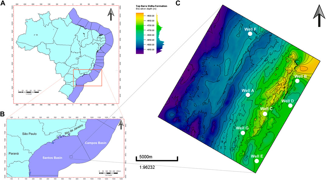
FIGURE 1. Map with the location of the seven wells analyzed.
The wells have a complete set of basic well logs from which we use caliper (CAL), density (RHOB), gamma-ray (GR), neutron porosity (NPHI), sonic (DT), along with NMR porosity and permeability, weight percentage curves (WPC) for carbonate, quartz-mica-feldspar and clays, water saturation and the HFU classified by Rebelo et al. (2022). Thin section images, technical reports, core and cuttings descriptions were also used when available. Well A also presents XRD data and, therefore, it represents the most reliable mineralogy data available when compared to the WPC, which is calculated by using Elemental Capture Spectroscopy (ECS) data.
To facilitate the comprehension of the methodological approach, this section is divided into four sequential parts. First, we present the aspect ratio pore type analysis and further extraction from thin section images by using the Fiji package. Then, we briefly explain how the classification to describe the main characteristics of the rock and pore types were performed. Next, we show how the sensitivity analysis was performed with commercial software to check how the parameters impact the model predictions by using a model that encompasses DEM and Gassmann’s theories (Gassmann, 1951). Finally, we explain the algorithm used (Kumar and Han, 2005) with the environmental trend extension proposal (Saberi, 2020). This step is necessary to calculate both aspect ratio (AR) and porosity proportions (PP) for each pore type in a pointwise manner. Figure 2 summarizes the main steps of the workflow proposed to evaluate these rocks.
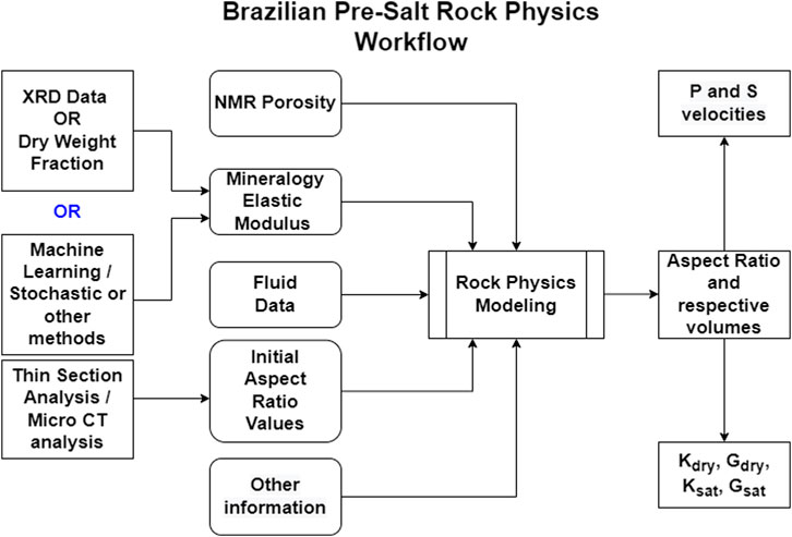
FIGURE 2. Workflow proposed for rock physics modeling of pre-salt carbonates in Brazil. Kdry, Ksat, Gdry, and Gsat, are the modeled bulk (K) and shear (G) moduli of dry and saturated samples, respectively. “Other information” are laboratory parameters that would help to constrain the modeling process, e.g., K and G moduli measured from laboratory experiments on core samples.
2.1 Pore type extraction analysis
We analyzed the available images from thin sections for well A to estimate aspect ratios to constraint our rock physics modeling. The Random Forest machine learning algorithm was applied to classify the pixels with pore or matrix indexes using the Fiji package on the open-source ImageJ software (Arganda-Carreras et al., 2007). Figure 3 presents the main steps performed toward the pore segmentation to obtain the necessary statistical parameters to estimate the aspect ratio for each pore type. The main steps are the following:
1) Define the appropriate scale to set pixel size in millimeters.
2) Create two classes (pores and matrix) by selecting pixels that are visible correspondent to either pores or matrix so as to have a training set.
3) Classify the remaining pixels using the training set as references.
4) Check consistency with the analyzed thin section image and set more training pixels if necessary to have a better classification result.
5) Create an 8-bit image and a binary image by setting a threshold.
6) Outline the pore boundaries on the binary image.
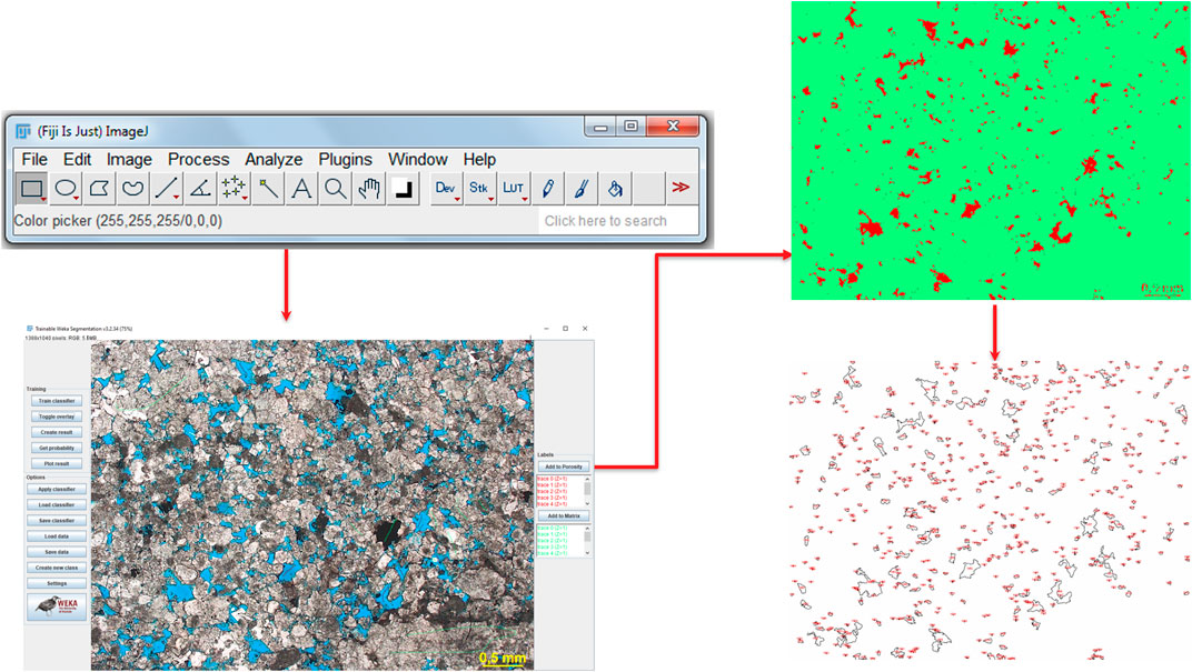
FIGURE 3. Fiji package and the main steps to segregate pores from the matrix on a thin section image.
After achieving pore segregation, the software provides statistical parameters such as area, perimeter, major and minor axes, the angle between axes, aspect ratio, etc.
2.2 Thin section images description
The wells count with a set of thin section images and description reports that were used to describe the main characteristics of the rock and its porous space. From this point on we will refer the available thin section images as thin sections only. The rocks were classified by Rebelo et al. (2022) following the system proposed by Gomes et al. (2020), which separates the rocks of the BVF into two groups: 1) in situ facies, which are classified into 12 categories according to the proportion of spherulites, shrubs, and mud and, 2) reworked facies that are classified according to the proportion of grain and matrix, following the classical scheme proposed by Dunham (1962).
Well A presents 139 thin sections of both in situ and reworked facies that were used to corroborate the rock physics model by comparing the identified pore types with the model predictions. The same procedure was performed in other wells which contain thin sections.
2.3 Sensitivity analysis
In order to perform the sensitivity analysis, we employed an oil-carbonate model to study the impact of the model’s parameters and ultimately predict P-wave (Vp) and S-wave velocities (Vs.). The model is based on the inclusion approach, and it uses an approximation of DEM introduced by Keys and Xu (2002) to compute the dry rock bulk and shear moduli. Fluid properties are computed with Batzle and Wang (1992) equations, and the saturated rock bulk modulus is computed using the classic Gassmann’s equations. This combination is effective and practical for the simulation of the low-frequency elastic responses of fluid saturated rocks (Mavko et al., 2009; Zhao et al., 2013). Also, as shown by some authors, the use of DEM for carbonates is more accurate than other methods such as self-consistent approximation or T-matrix (Vanorio et al., 2008; Misaghi et al., 2010). Finally, Vasquez et al. (2019) results suggest that Gassmann’s equations may be applied in the Brazilian pre-salt carbonates. For a further and detailed analysis of the equations, see, e.g., Misaghi et al. (2010).
The sensitivity analysis is performed by fixing all parameters and varying one to check its impact through the model templates. One example is analyzing the impact on velocity predictions by modifying a certain parameter in a cross-plot between compressional velocity (Vp) and total porosity obtained from Nuclear Magnetic Resonance (NMRtt). Supplementary Figure S1 shows an example of the variation of water saturation within the system. The analyses were performed considering parameters such as mineralogy volumes (calcite, dolomite, quartz and clays), aspect ratio (reference, stiff and compliant pore types) and their respective volumes, water saturation, among others. The elastic moduli and density of minerals are from Mavko et al. (2009), except clays, that are from Vasquez et al. (2019).
2.4 Kumar and Han algorithm extended by saberi
Kumar and Han (2005) published a well-known algorithm that calculates pore aspect ratios and their respective volume fractions using a pointwise approach for each available depth data. The authors verified the effectiveness of the method by studying 52 carbonate samples of 22 wells from different fields in the world through the comparison between measured and calculated velocities. Several authors used this algorithm in carbonates, such as Xu and Payne (2009), Mirkamali et al. (2020) and Saberi (2020). The algorithm steps (sensu Mirkamali et al., 2020) can be subdivided as follows:
1) For φreference, φcompliant, and φstiff calculate Vp using time-average (TA), lower and upper Hashin-Shtrikman for a given bulk porosity.
2) Use DEM for given bulk porosity and an initial estimate of AR (αR = 0.1 for reference, αS = 1 for stiff and αC = 0.01 for compliant) to calculate the VP of the rock. VPDEM = (K0, μ0, α, φb), where K0 and μ0 are matrix bulk and shear modulus.
3) If (VPDEM(α)—VP (α))2 > ε, then α = α ± δα, where ε is the chosen error value.
4) Take the aspect ratio (α) for each pore type when (VPDEM(α) –VP (α))2 < ε.
5) Obtain aspect ratios for reference, compliant and stiff pores as αreference, αcompliant and αstiff, respectively.
The algorithm follows a similar pattern for the pore type volume calculation and starts with the premise that all porosity relies upon the reference pore type. These steps are as follows:
6) Compare measured velocity with VPreference calculated from DEM. If VP > VPreference(DEM), then α1 = αreference, α2 = αstiff, φ1 = φtotal, φ2 = 0, otherwise, if VP < VPreference(DEM), alpha 2 becomes α2 = αcompliant. In other words, when the measured velocity is larger than the modeled velocity, we adjust the reference and stiff porosity volumes and, when the measured velocity is lower than the modeled velocity, we adjust reference and compliant porosity volumes.
7) Recalculate VPDEM, and if (VPDEM(α)—VP (α))2 > ε, then instead of incrementing alpha as explained in step 3, we increment phi as φ = φ ± δφ.
8) When (VPDEM(α)—VP (α))2 ≤ ε, then the increments stop, and we take this value and obtain porosity percentage for each aspect ratio αreference, αcompliant and αstiff, respectively.
This procedure can model only two pore types for each depth point, i.e., αreference and αstiff or αreference and αcompliant. Therefore, the same logic applies to porosity volume distribution among the distinct pore types. To overcome this limitation, Saberi (2020) proposed an extension to this approach with the addition of a new reference curve, called the environmental trend curve, to perturb the time-average response and expand the number of pore aspect ratios per depth sample analyzed. This ET curve brings a geologically driven approach to calibrate the determined pore models from the Wyllie TA being based on the actual subsurface microstructure (Figure 4).
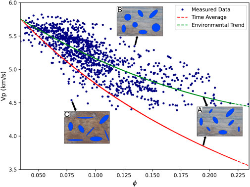
FIGURE 4. Example of using two reference curves to perform the three pore-type modeling for each depth point. Note that reference pore types are always included in the modeling process, while stiff pores come from positive deviations from the red and green curves, and compliant pores come from negative deviations. “A” indicates a mixture of reference and compliant pore types from the ET curve (green) and a mixture of reference and stiff pore types from the TA curve (red). “B” indicates a mixture of reference and stiff pore types from both curves, and “C” indicates a mixture of reference and compliant pore types from both curves.
An easy way to understand how it is possible to model three pore types for each depth point is to visualize a data point located between the red and green curves. While a positive deviation (greater velocities) from the TA curve will model a mixture of reference and stiff pores, the same point will have a negative deviation from the ET curve and, therefore, will model a mixture of reference and compliant for the same point.
As an upgrade to this approach, we inserted XRD and saturation curves into the workflow for well A, so both aspect ratio and porosity proportion use different bulk moduli, shear moduli and density values for each depth due to the unique combination of mineralogy and fluid data. In addition, we assumed that the difference between the total mineralogy (100%) and the sum of calcite, dolomite and quartz corresponds to clays, since they are not present in the XRD data and are a key part of the complex pre-salt mineralogy (Gomes et al., 2020; da Silva et al., 2021) (Supplementary Figure S2).
The other wells did not present XRD, and, therefore, we used only the available weight percentage curves (WCAR, WQFM and WCLA) from ECS. The WCAR curve was segregated into calcite and dolomite by performing sensitivity analysis within distinct proportions and comparing which proportion of calcite and dolomite gives a better approximation between the density calculated and measured.
3 Results and discussion
3.1 Pore type extraction analysis
Supplementary Figure S3 shows nine histograms to demonstrate statistical parameters extracted from thin sections analyzed throughout well A. Pore classification, number of pores, minimum, maximum, mean, and standard deviation values are shown. For this well, 38 thin sections were used covering ∼162 m of the BVF, where 1846 pores were identified. Supplementary Table S1 summarizes some parameters obtained for each depth.
It is possible to note from the histograms that most pore types are located between 0.2 and 0.8, falling basically on the reference-stiff pore type literature values range. The histograms, generally, do not show a trimodal or bimodal behavior and, therefore, it is not easy to segregate compliant, reference, and stiff pores. As shown in Supplementary Table S1, the average for the entire well is 0.48 and the standard deviation is 0.17, which gives an interval of 0.31 up to 0.65. When we consider an area weight, this number falls to 0.46, which is close to the simple average. The weighted average must be analyzed with care because cracks may cause a great impact on velocity, as pointed out in several works, such as Anselmetti and Eberli (1993). Compliant pores are difficult to segregate, and 3-D micro-computed tomography (micro-CT) analysis may provide better results. For the sake of the following discussion, the reader must be aware that here we are mentioning only macropores and, thus, micropores will not be considered.
Some limitations in performing this analysis were present due to the lack of better resolution for the available images. For example, the thin section from Figure 5 presents a resolution of 487 × 365 pixels. If we consider the minimum detectable Y dimension as one pixel and divide it by the size of the image along the X dimension, we obtain a minimum detectable aspect ratio of 2.05 × 10⁻³, approximately. For this thin section, 1 mm equals 170 pixels. Care must be taken when assessing the thin section images due to what we refer to here as “transition pixels” between porosity (blue) and matrix (rest of the image). Usually, these pixels present intermediate color values, and the algorithm sometimes classifies them as matrix and sometimes as porosity. Cementation with white or clear colors also may harm the classification.
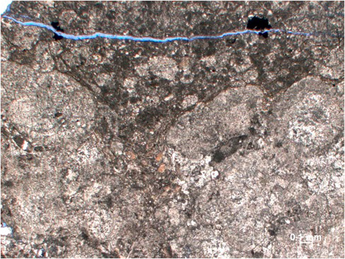
FIGURE 5. Thin section image from well A (depth = 4,950.3 m).
Supplementary Figure S4 exemplifies pore segregation (A) and best-fit ellipses (B) used for extracting statistical parameters such as aspect ratio. The ellipse in (B) considers the angle between the axes and, thus, the aspect ratio is clearly higher than reality. This proves that this method is accurate enough for stiff and reference pores but is not always reliable for compliant pores or cracks. For this last case, it can provide an idea of the aspect ratio but not the exact results.
Although this approach presents limitations, in the lack of micro-CT images, this method can be used to obtain the necessary initial guesses for stiff and reference pore types from thin sections.
3.2 Sensitivity analysis
In our oil-carbonate model, calcite is always present since it is the most abundant pre-salt carbonate mineral. The clay contents were assumed as the difference between one hundred percent and the total amount of calcite, dolomite, and quartz. Table 1 provides the main parameters used within the model.
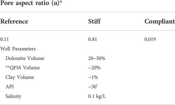
TABLE 1. Main parameters used in the “Oil-Carbonate Model”. (*) minor to major axis ratio; (**) QFM stands for quartz, feldspar, and mica, but here we consider that it is only quartz because this is the most common mineral among those three in the pre-salt.
Figure 6 shows four results: (A) the variation of dolomite volume, (B) the variation of the aspect ratio for the reference pore type, (C) the variation within the volume present in the reference pore type, and (D) the volume present in compliant pore type. As dolomite volume increases, there is a positive impact on velocity predictions, as expected, since this mineral presents a higher elastic modulus when compared to the rest of the system, i.e., calcite, quartz, and clay. More important are the values chosen for the aspect ratios, e.g., for the reference pore type, inserted in the model as Figure 6B shows on the upper right, which would change data interpretation dramatically when considering the impact of these parameters, as pointed out by Eberli et al. (2003). For example, if we use 0.2 for reference as an input for this model, we expect to have a considerable amount of compliant pores within these rocks, which does not match with what we have seen in thin sections. Figures 6C,D show the volume variation of reference and compliant pore type, respectively. If we look at the end of the curves (at 20% porosity), it is possible to see that a difference of 5% in compliant volume would impact velocity by around 10%. This has virtually the same impact if we consider a variation from 50 to 80% in reference volume at the same porosity point. This shows the importance of obtaining these parameters in a pointwise manner.
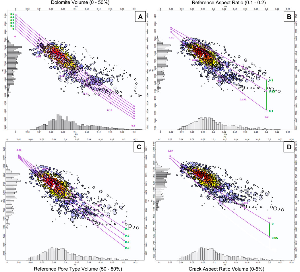
FIGURE 6. Sensitivity analysis examples. In (A) it is possible to see how the increase of dolomite impacts the velocity predictions positively. Notice in (B) how the choice of reference aspect ratio dramatically affects our dataset’s interpretation. (C) represents how the increase in volume present in the reference pore type negatively affects velocity. (D) shows the volume of compliant pore type, which has a stronger effect with lesser volume variation.
As mentioned before, we used other parameters, and the results point out that pore type aspect ratio and volume plus mineralogy represent the most sensible parameters within the system. Therefore, strong control of these parameters is fundamental to obtain reliable results when modeling P and S-waves in different scenarios. Also, as porosity increases, the impact of mineralogy matrix in the rock elastic behavior decays in importance in relation to pore aspect ratio and volume, as expected. This behavior was also observed by Dias et al. (2021).
3.3 Aspect ratios and their respective volumes along the well logs
This section presents detailed results for wells A and B, while the other five wells (C, D, E, F and G) will be briefly summarized.
3.3.1 Well A
Well A has the most complete dataset and, additionally, this well was the only one with XRD data through BVF and, therefore, the most reliable to be used for tests and calibration. Thus, this well will be presented in more detail.
The data in the cross-plot between compressional velocity against porosity remains inside the Hashin-Shtrikman upper and lower bounds indicating that XRD mineralogy is reliable, as expected.
As explained before, the facies described here follow Gomes et al. (2020) proposed classification for the BVF, and Dunham’s classification was used to describe the reworked facies as explained in the methodology section. Based on these classifications, this well presents mainly spherulitestone-shrubstone variations, grainstones, packstones, mudstones and wackestones.
The model prediction shows that this well mainly presents reference pore types, with stiff pores being secondary in importance (Figure 7). This happens for all wells described here, and it was expected since the available 139 thin sections for this well show mainly interparticle porosity. Also important are intraparticle, moldic and vuggy pore types, with rare presence of microfractures. Thin sections and cores were described by using the available images, and the conclusion remains the same, i.e., our model provides reliable information for this well (Figure 8). The measured and the predicted Vp by the model present a good match, and the correlation between these curves is 0.979 with a normalized root mean squared error (NRMSE) of 0.07.
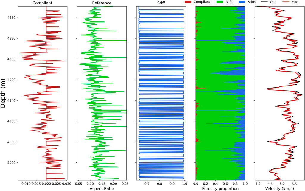
FIGURE 7. Aspect ratios, porosity proportions and measured versus predicted velocity curves obtained from Kumar-Han-Saberis pointwise method. Obs means the observed (measured) well log curve and Mod means the modeled curve.
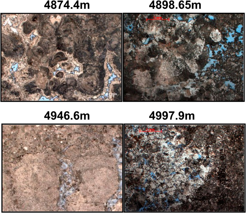
FIGURE 8. Four thin section images showing mineral and pore system characteristics of well A. Numbers indicate depths.
Figure 9 shows results for the porosity proportions for the three pore types and most part of the porosity is predicted to be within the reference pore type with stiff subordinated to it. The figure shows basically a mirror image between these two pore types since compliant pores have low porosity values. This is common for the studied wells. Since Kumar and Han approach starts with the assumption that most part of the volume will be within reference pores, and then the algorithm makes an adjustment for the other pore types, usually stiff and compliant volumes vary greatly and, thus, statistical parameters such as mean and standard deviation are not useful. Therefore, we will present these values only for reference pores and maximum values for the other two pore types. The minimum values are virtually zero for all pore types since it is dependent on the NMR log, i.e., when total porosity is 1%, this will be the value to be adjusted and distributed among the three pore types. For this well, reference pores volume presents an average of 8.5% and a maximum value of 27.9%, with a standard deviation of ±3.3%. Stiffs present a maximum value of 10.0%, while compliant pores show a maximum of 2.0%.
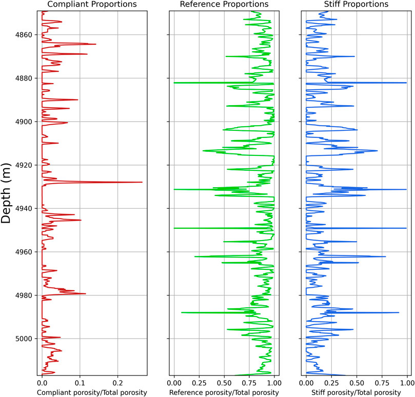
FIGURE 9. Porosity proportions obtained from Kumar-Han-Saberi’s pointwise method for each pore type. Note that the x-axis scale is larger for compliant pores.
The ternary plot in Supplementary Figure S5 shows data distribution in terms of calcite, dolomite, and quartz contents. In terms of volume, the mineralogy distribution follows this order but, we must emphasize the importance of dolomite present as micrite matrix, cementation and dolomitization in some thin sections. Additionally, the plot shows the distribution of the R35 Flow Unit’s classification (Aguilera, 2002). From HFUs 1 to 4, this classification presents better porosity-permeability relation and HFUs 2 and 3 are the most abundant. Circle size indicates free fluid content and, hence, it is possible to check that HFU 3 is the most important unit in terms of permo-porosity quality and, volumetrically, presents a concentration within the calcite axis.
Finally, we tried to relate the calculated pore type volumes with the HFUs classification in a 3-D view (Figure 10). As the reader may acknowledge, there are white parts which indicate an overlap between data (mainly between units two and three). We can observe from this figure that the best HFUs (3 and 4) are distributed in a higher combined value between reference and stiff pores when compared to HFUs 1 and 2. Especially, HFU 2 presents higher compliant porosity proportion values, while HFU 3 advances towards the stiff axis.
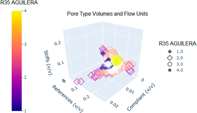
FIGURE 10. Distribution of pore type volumes and R35 Aguilera hydraulic flow units for well A.
Hence, the best scenario for this well in terms of permo-porosity quality, indicates a combination of HFU 3, reference pores, stiffs being secondarily in importance, and calcite content with dolomite subordinated to it. As HFU 3, HFU 2 also shows similar free fluid content and compliant pores or cracks may act as connectors to reference and stiff pores as it will be discussed later.
3.3.2 Well B
The predominant facies of well B correspond to the intercalation between grainstones and packstones. Less frequent but also present are wackestones, spherulitestones, shrubstones, mudstones, spherulitic-mudstone, spherulitic-shrubstone and muddy-spherulitestone.
This well does not present XRD data, which brings more uncertainty within the mineralogical scenario when compared to well A. Therefore, we used the available weight percentage curves WCAR, WQFM and WCLA. This provides a less accurate perspective compared to XRD data, where calcite, dolomite and quartz are separated, although results for this well prove that this data is also reliable as it will be discussed later.
There are 87 thin sections available within the interval between 4,815 and 4,849 m. We did not consider the first 10 m of this well due to unreliable well log values readings (indicated by caliper and other curves). Figure 11A shows a thin section example from 4,834.8 m, where porosity volume distribution shows a similar pattern described in well A. The pores in this thin section are consistent with the model predictions, i.e., it shows a mixture of reference and stiff pore types. Some peaks of stiff pores are observed between 4,950 and 5,000 m, but care must be taken since there are no thin sections available that cover this last interval.
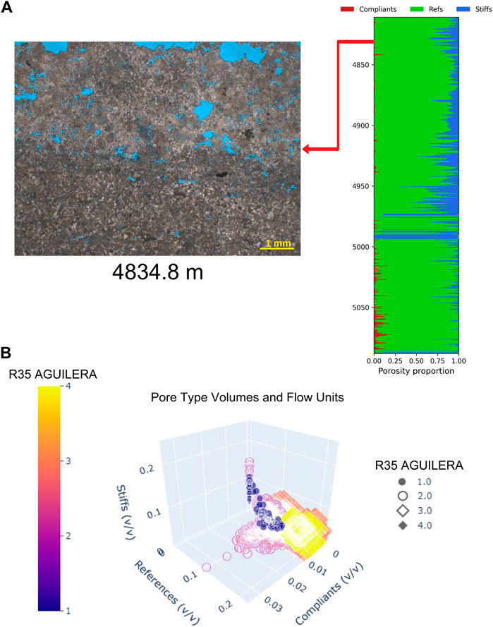
FIGURE 11. (A) Thin section from 4,834.8 m (well B) showing interparticle and vuggy porosity which is consistent with the model prediction of being mainly reference and stiff pores. (B) Distribution of pore type volumes and R35 Aguilera hydraulic flow units.
The velocity predicted by the model shows a good match with the measured Vp (correlation of 0.97), with an NRMSE of 0.09. Similar porosity proportion curves as shown in Figure 9, were calculated for this well and show that reference pore volume presents an average of 10.8% and a maximum value of 21.4%, with a standard deviation of ±3.9%. Stiff and compliant pores show a maximum value of 14.5% and 3.3%, respectively.
Figure 11B displays the relation between calculated pore type volumes with the HFUs classification in a 3-D view. Here, HFUs 2 and 3 predominate, although the occurrence of HFU 4, the best one in terms of porosity-permeability, is relevant. HFU 2 is more widespread through the three axes and this unit advances towards higher compliant porosity values when compared to the other units. Also, it is possible to observe that the best HFUs (3 and 4) are distributed in a higher combination between reference and stiff pores when compared to HFUs 1 and 2. Unit 1 is predominant and, surprisingly, shows a subgroup well distributed within the stiff axis but, when compared with the other units, shows lower reference values. This is probably an indication of low permeability of unconnected moldic and/or vuggy pores.
Hence, the best scenario for this well, in terms of permo-porosity quality, indicates a combination of HFUs 3 and 4, high porosity distribution in reference pores and carbonate content with quartz subordinated to it.
3.3.3 Wells C, D, E, F and G
Wells C and E present thinner intervals of BVF when compared to other wells, i.e., less than 60 m. All wells show a good correlation between the Vp measured and the Vp predicted (>0.9) and low NRMSE values (≤0.08).
In well C, grainstones are predominant and are intercalated with variations of spherulitestones and shrubstones. The 25 thin sections analyzed show that this well presents mainly interparticle, moldic and vuggy porosity. Intraparticle porosity is less present and just few microcracks were described around 4,740 and 4,760 m. Our model was able to predict compliant pore type close to both depths shown by red fills (Supplementary Figure S6).
Well D is composed mainly of grainstones and has 71 thin sections described, which show that cementation by dolomite, quartz, silica, and calcite occurs. Also, volcanic rock fragments and silica grains play an important role. This is also denoted by the increasing WQFM content. Thus, this well presents a peculiar mineralogy when compared to the others described. Therefore, results for this well must be interpreted with care since this is an inclusion model. In terms of porosity-permeability, the best scenario combines HFUs 3 and 4 with the distribution mainly on the reference and stiff axes.
Furthermore, the more prominent presence of HFU 4, with high values of free fluid, may suggest that, in this well, compliant pores and cracks do not necessarily act as connectors for reference and stiff pores.
Well E shows mainly references with stiffs secondarily to it, but around 4,842 m, this pattern is inverted up to the end of BVF. Compressional velocity presents a faster trend denoting a stiffer rock framework from this interval on. Compliant pores appear in some parts of the well, mainly from 4,820 to ∼4,835 m and, porosity proportion distribution also follows this pattern with stiff volumes predominating at the end of the well. Unfortunately, the available 41 thin section for this well were focused on texture and its main constituents and not on pore types. However, it was possible to see compliant pore types (red circles) around 4,834 m (Figure 12).
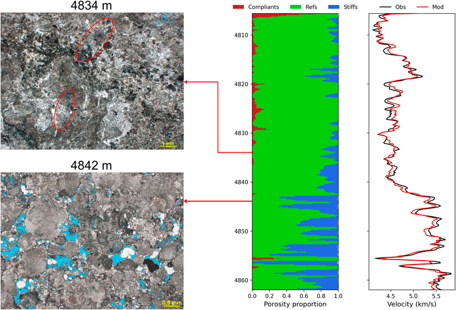
FIGURE 12. Thin section images denoting an increase in stiff pores predicted in the model starting around 4,842 m depth (blue color). Note how Vp also increases its trend, which indicates a stiffer rock framework. The compliant’s prediction follows the strong decrease in velocity. “Obs” means the observed (measured) well log curve and “Mod” means the modeled curve.
This well also presents a mirror image of pores between references and stiffs but, differently than the previous ones, there are some high peaks of stiff porosity along the well. In terms of HFUs, it presents mainly HFU 3 with HFU 2 subordinated to it. Both are distributed within the same pattern around the three axes and unit three shows higher reference volume values. HFU 4 shows the bigger stiff values and lower compliant values, while HFU 1 is basically null. Therefore, the best scenario in terms of porosity-permeability combines units three (and four secondarily) with a distribution on the three axes with an important contribution from the stiff axis. This might suggest that, in the same way as seen in well D, stiff pores seem to be connected but, distinctly from the previous well, it seems that also compliant pore types contribute to permeability.
Well F presents some points outside the Hashin-Shtrikman upper bound. Given properly mineralogy and fluid content, in theory, this should not happen but, descriptions in 68 thin sections show the presence of dolomite, crystalline carbonate and rare cementation by pyrite and barite. Thus, it is justifiable that few points surpass this bound, but results must be analyzed with this in mind. The most important lithologies are grainstones, stromatolites, spherulitites and laminites. In terms of HFUs, this well presents mainly HFUs 1, 2, and 3. HFU 2 in this well also shows that compliant pores may act as connectors.
Well G is composed mainly of spherulitites (and variations with dolomite or clay) and grainstones. With less frequency, there are stromatolites, laminites and rudstones. Cementation by dolomite, quartz and calcite is also common within these rocks. Anhydrite is not described within the 34 thin sections but appears in the weight percentage curves (WANH) and it was considered in the modeling process. For this dataset, there is no data outside the Hashin-Shtrikman bounds. Results show that reference pores are predominant while stiffs show some peaks along the well. Compliant pores appear with low values, but it presents a peak within a strong drop in Vp around 5,220 m. In terms of HFUs, this well presents a mixture of HFUs 1, 2 and 3, being the last two more abundant. HFU 4 is virtually absent, and it is not important along this well. HFU 2 is better distributed along the axes, while units one and three are more concentrated in reference and compliant axes showing low stiff values, when compared to the wells described here. Hence, this well presents the worse scenario in terms of porosity-permeability.
As stated in Dvorkin (2020), we can portray rock physics as a “velocity-porosity-mineralogy-fluid” science. In pre-salt rocks, mineralogy and pore types play a major role in the elastic behavior of these carbonates as sensitivity analysis shows. While stress has a significant impact on clastic rocks, in carbonates the effect is not as important as compliant cracks. The author shows that velocity hardly changes, e.g., in samples from the Ekofisk field, in the North Sea, when cracks are absent. In fact, studies show that mineralogy, rock framework and pore structure, which are a function of the depositional environment and diagenesis (cementation, dissolution, and recrystallization), have a bigger impact on the elastic rock behavior in carbonates.
One of the main difficulties in applying this method is obtaining reliable mineralogical curves, especially, when dealing with clay-rich intervals. Tests with calculated shale and stevensite curve volumes were performed with wells that did not present mineralogy data along with the available dataset. Results showed that shale and/or stevensite curves seem to be overestimated since data surpass the Hashin-Shtrikman bounds, and this has been a difficult problem to solve. In other words, the excess of clays in the system brings the upper bound to lower velocities, which does not seem plausible. For example, de Oliveira et al. (2021) tested four algorithms with pre-salt carbonate rocks to obtain the following minerals: calcite, dolomite, quartz, clay, K-feldspar, plagioclase, and pyroxene. According to the authors, the clay model is influenced mainly by Mg, Na, LOI, carbonates, quartz, and secondarily by Si and Ca, reflecting great variation both in the chemical composition and their depositional environment. Another finding is that by using only chemical elements the models for clay and dolomite show more noise.
Regarding the importance of microporosity, Zielinski et al. (2018) studied the coquina pore system from Morro do Chaves Formation, in the Sergipe-Alagoas basin, by using micro-CT techniques and one of the findings was that permeability in vugular pores came from microporosity acting as connectors. In well E, although we cannot see microporosity, there is a clear example of cracks acting as connectors between other pore types (Figure 13). This also may happen on the microscale with microcracks acting as corridors to bigger pores.
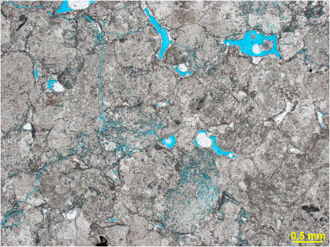
FIGURE 13. Thin section image showing that compliant pores may act as connectors between other pores of the pore system.
Basso et al. (2021), highlight the importance of pores below 40 μm in the BVF. The authors discuss that even for samples dominated by macroporosity, pores below this value comprise more than half of the pore system of the studied samples and, thus, consist of a fundamental part of the pore system connectivity.
The results from the 3-D plots show, in some cases, that bigger values of free fluid are also present within HFUs that advance towards the compliant axis denoting that these may act as connectors to references and stiffs pore types, or in a geological perspective, fractures and microfractures are connecting interparticle, moldic and vugular pores.
Scenarios vary strongly from well to well reflecting how complex is the relationship between key parameters such as porosity, pore types, mineralogy, fluid, permeability, and diagenesis.
It is worth mentioning that we performed preliminary tests by using the S-wave to obtain the pore type distribution along with the depth. Preliminary results show that the S-wave seems to be more sensitive to compliant pore type identification. In other words, for certain cases, while some compliant pores do not appear in the modeling process by using the P-wave, they are identified when using the S-wave. Studies point out that P and S-waves are affected differently by the pore geometries, and while the results are expected to be slightly different from each other, they should be consistent (Fournier et al., 2011; Wang et al., 2011). However, it must be emphasized that the modeled curve tends to present a lower correlation when compared to the P-wave case. Therefore, the study by using S-waves or the combination of both P and S-waves must be explored in the future as proposed by Mirkamali et al. (2020).
3.3.4 XRD and WPC results comparison - Well A
To check the reliability of using WPC mineralogy for the other wells (B to G), instead of XRD, only present in well A, we applied the same workflow to compare both datasets. Figure 14 summarizes the main results for reference aspect ratio and volumes for each pore type.
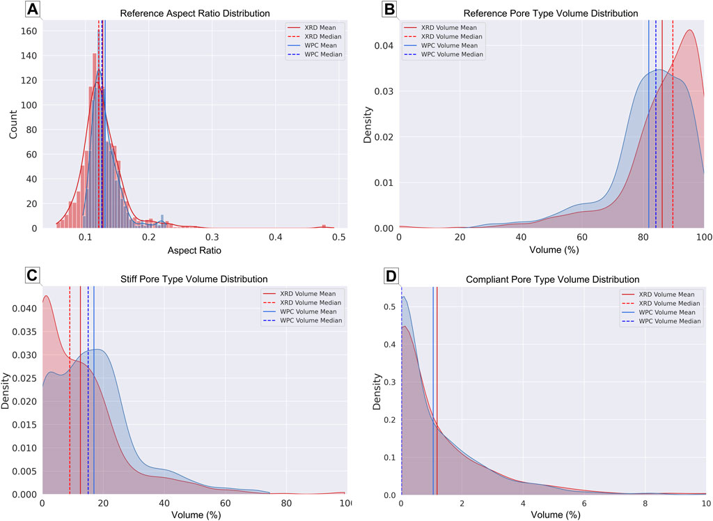
FIGURE 14. (A) Histogram and kernel density function with mean and median (dashed lines) for XRD and WPC in red and blue, respectively. XRD shows a greater variability as expected. (B), (C) and (D) Reference, stiff and compliant pore type volume distributions showing similar values for both cases. Note that reference volume is lower for the WPC in (B) and, it is compensated by the higher distribution within stiff pores in (C).
The Kernel Density Model (KDE) model for the XRD presents mean aspect ratio of 0.127 and median of 0.121, while the KDE model for the WPC shows a mean of 0.131 and median of 0.126. Both scenarios show a unimodal distribution and, as expected, the XRD has a greater variability than the WPC since it is more precise (Figures 14A). While the XRD provides the volumes for calcite, dolomite and quartz, the three main minerals within the system, the WPC does not separate carbonate minerals (WCAR), quartz, feldspar and mica (WQFM), and clay mineralogy (WCLA). Therefore, it is expected a higher variation in the first case.
The KDE models for stiff and compliant pore aspect ratios present insignificant differences and are not shown in Figure 14. While the medians for stiff pores present similar values, the mean is affected because of the bimodal distribution of these pore types. The median for both scenarios is around 0.64, whilst the mean is 0.80 and 0.72, respectively. For the compliant aspect ratio, both the mean and median are around 0.019 and 0.02, respectively. Considering that these KDE functions are similar for both cases, it is more interesting to analyze their volume fraction distributions.
The KDE XRD model for reference pores shows volume mean and median of 86.2% and 89.7%, respectively, while the WPC model shows a mean volume of 81.8% and a median of 84.1%. The difference is compensated by the allocation of more stiff pores volume for the WPC scenario, whilst compliant pores volume remain virtually the same (Figure 14B).
Stiff volume fractions present higher values for the WPC case. This was expected because the reference pore models show an opposite behavior. The differences for the mean and median values are 12.5% (XRD) to 17.0% (WPC) and 9.0% (XRD) to 15.0% (WPC), respectively (Figure 14C). The compliant volume fractions present a similar distribution in both scenarios, with means around 1.2% and 1.1%, and medians of 0.018% and 0.019% for XRD and WPC, respectively (Figure 14D). Supplementary Table S2 summarizes the difference quantification between XRD and WPC results. Cataldo et al. (2022), extended this analysis comparing XRD versus a fixed mineralogy scenario based on published literature in the Brazilian pre-salt.
4 Conclusion
We presented a workflow that integrates several methods to obtain a depth-variant distribution of pore types and their respective volumes within the complex Brazilian pre-salt carbonates. As explained before, one of the goals of this work was to obtain the distribution of these parameters for the BVF because they strongly impact the velocity behavior of seismic waves. A sensitivity analysis show that the use of fixed values instead of depth-variant values brings significant uncertainties into the velocity modeling.
The analysis pointed out that the most sensible parameters within the system are the aspect ratio and mineralogy, i.e., they have a bigger impact on the velocity predictions. Water saturation has a grown impact as porosity becomes higher obviously but, this happens mainly between 75–100% of water saturation and, therefore, when compared to aspect ratio and mineralogy, its impact is secondary. Thus, if we have good control over mineralogy, porosity, and saturation, then we need to adjust the aspect ratio and their respective volumes in a depth-variant manner, in order to get reliable P and S-wave modeled curves.
Another way to improve the reliability of the model would be to separate the different types of clay present in pre-salt, e.g., stevensite, smectite, kerolite and saponite but this remains a difficult task.
Therefore, the main concern for reliable predictions should be to acquire more information on fluid mixture, mineralogy and pore types by studying thin sections and/or micro-CT images, especially for the last two parameters. This would provide the main constraints for the geological scenario of the model, and, consequently, the prediction results should be as trustworthy as possible.
Results suggest that compliant pore types may act as connectors between reference and stiff. Hence, it is important to identify them because they may carry fluid to pores with bigger storage capacity.
By using WPC instead of XRD for well A, there are no significant differences between the calculated reference aspect ratios. While the first shows a mean value of 0.131, the second presents a mean of 0.127, i.e., an overestimation of only 3.15% in average, considering that the scenario with XRD is our reference. Stiff aspect ratio is underestimated by 10%, while the difference in crack aspect ratio is virtually zero. The volume proportions present an underestimation of 4.4% for reference and 0.1% for cracks, and an overestimation of 4.5% for stiffs in average. Preliminary studies indicate that S-wave seems to be more sensitive to compliant pores. As shown in previous studies, P and S-waves may be affected differently by the pore geometries, so the use of both could bring slightly different results, which may highlight compliant porosity not identified by using the compressional wave alone.
Data availability statement
The original contributions presented in the study are included in the article/Supplementary Material, further inquiries can be directed to the corresponding author.
Author contributions
RC: project conception, data processing and analysis, data interpretation, writing. EL: project conception, data processing, writing. NM: data interpretation, writing. TR: data interpretation, writing.
Funding
This research was carried out in association with the ongoing R&D project registered as ANP nº CW266675, “Integrated multi-scale analysis of pre-salt carbonate rocks for the characterization and prediction of reservoir properties” (Unicamp/Shell Brasil/ANP), sponsored by Shell Brasil under the ANP R&D levy as “Compromisso de Investimentos com Pesquisa e Desenvolvimento”.
Acknowledgments
The authors would like to thank the Shell research team for all the support, comments and suggestions to improve the manuscript, the Geophysics Laboratory of the Institute of Geosciences, UNICAMP, for providing the necessary computer resources, and GeoSoftware for providing academic software licenses. RC thanks CNPq for his scholarship (process number 140342/2019-2). EL thanks CNPq for his productivity grant (process number 311491/2019-7).
Conflict of interest
The authors declare that the research was conducted in the absence of any commercial or financial relationships that could be construed as a potential conflict of interest.
Publisher’s note
All claims expressed in this article are solely those of the authors and do not necessarily represent those of their affiliated organizations, or those of the publisher, the editors and the reviewers. Any product that may be evaluated in this article, or claim that may be made by its manufacturer, is not guaranteed or endorsed by the publisher.
Supplementary material
The Supplementary Material for this article can be found online at: https://www.frontiersin.org/articles/10.3389/feart.2022.1014573/full#supplementary-material
References
Aguilera, R. (2002). Incorporating capillary pressure, pore throat aperture radii, height above free-water table, and winland r35 values on pickett plots. AAPG Bull. 86 (4), 605–624.doi:10.1007/s00531-020-01932-7
Anselmetti, F. S., and Eberli, G. P. (1999). The velocity-deviation log: A tool type and permeability in carbonate drill holes from sonic and porosity or density logs. AAPG Bull. 83, 450–466.
Arganda-Carreras, I., Kaynig, V., Rueden, C., Eliceiri, K. W., Schindelin, J., Cardona, A., et al. (2017). Trainable Weka segmentation: A machine learning tool for microscopy pixel classification. Bioinformatics 33 (15), 2424–2426. doi:10.1093/bioinformatics/btx180
Basso, M., Belila, A. M. P., Chinelatto, G. F., Souza, J. P. d. P., and Vidal, A. C. (2021). Sedimentology and petrophysical analysis of pre-salt lacustrine carbonate reservoir from the Santos Basin, southeast Brazil. Int. J. Earth Sci. 110, 2573–2595. doi:10.1007/s00531-020-01932-7
Batzle, M., and Wang, Z. (1992). Seismic properties of pore fluids. Geophysics 57, 1396–1408. doi:10.1190/1.1443207
Boyd, A., Souza, A., Carneiro, G., Machado, V., Trevizan, W., Santos, B., et al. (2015). Presalt carbonate evaluation for Santos Basin, offshore Brazil. Petrophysics 56, 577–591.
Brie, A., Johnson, D. L., and Nurmi, R. D. (1985). “Effect of spherical pores on sonic and resistivity measurements,” in Proceeding of the 26thAnnual Logging Symposium, Dallas, Texas, June 17–20, 1985 (Society of Professional Well Log Analysts).
Buchheim, H. P., and Awramik, S. M. (2014). Stevensite, oolite, and microbialites in the eocene green river formation, sanpete valley, uinta basin, uta. Pittsburgh: AAPG Search & Discovery.
Castro, T. M., and Lupinacci, W. M. (2022). Comparison between conventional and NMR approaches for formation evaluation of presalt interval in the Buzios Field, Santos Basin, Brazil. J. Petroleum Sci. Eng. 208, 109679. doi:10.1016/j.petrol.2021.109679
Castro, T. M., and Lupinacci, W. M. (2019). “Evaluation of fine-grains in pre-salt reservoirs,” in 16th International Congress of the Brazilian Geophysical Society and EXPOGEf, August 19-22, 2019, Rio de Janeiro.
Cataldo, R. A., Leite, E. P., and Mattos, N. H. S. (2022). “Impact of mineralogy on rock physics modeling: A Brazilian presalt case study,” in Second International Meeting for Applied Geoscience & Energy (Society of Exploration Geophysicists and American Association of Petroleum Geologists), August 28-September 1, Houston, TX 2333–2337. doi:10.1190/image2022-3751121.1
Clarke, D., Blaauw, M., Guha, J., Sansal, A., Unaldi, M., and Zhang, B. (2021). Novel machine learning workflow for rock property prediction in the geologically complex pre-salt Santos Basin, Brazil. Denver: SEG Technical Program Expanded Abstracts, 1520–1524.
da Silva, M. D., Gomes, M. E. B., Mexias, A. S., Pozo, M., Drago, S. M., Célia, R. S., et al. (2021). Mineralogical study of levels with magnesian clay minerals in the Santos Basin, aptian pre-salt Brazil. Minerals 11, 970. doi:10.3390/min11090970
de Carvalho, M. D., and Fernandes, F. L. (2021). “Pre-salt depositional system: Sedimentology, diagenesis, and reservoir quality of the Barra Velha Formation as a result of the Santos Basin tectono-stratigraphic development,” in The super giant petroleum system of the pre-salt from the Santos Basin, Brazil: AAPG memoir 124. Editors Marcio R. Mello, Pinar O. Yilmaz, and Barry Katz.
de Oliveira, L. A. B., Custódio, L. F. N., Fagundes, T. B., Ulsen, C., and de Carvalho Carneiro, C. (2021). Stepped machine learning for the development of mineral models: Concepts and applications in the pre-salt reservoir carbonate rocks. Energy AI 3, 100050. doi:10.1016/j.egyai.2021.100050
Dias, J., Lopez, J. L., Velloso, R., and Perosi, F. (2021). A workflow for multimineralogic carbonate rock physics modelling in a bayesian framework: Brazilian pre-salt reservoir case study. Geophys. Prospect. 69 (3), 650–676. doi:10.1111/1365-2478.13060
Dou, Q., Sun, Y., and Sullivan, C. (2011). Rock-physics-based carbonate pore type characterization and reservoir permeability heterogeneity evaluation, Upper San Andres reservoir, Permian Basin, west Texas. J. Appl. Geophys. 74 (1), 8–18. doi:10.1016/j.jappgeo.2011.02.010
Dunham, R. J. (1962). “Classification of carbonate rocks according to depositional texture,” in Classification of carbonate rocks. Editor W. E. Ham (Tulsa: Am. Assoc. Pet. Geol. Mem), 1, 108–121.
Dvorkin, J. (2020). “Rock physics: Recent history and advances,” in Geophysics and ocean waves studies (London IntechOpen).
Eberli, G. P., Baechle, G. T., Anselmetti, F. S., and Incze, M. L. (2003). Factors controlling elastic properties in carbonate sediments and rocks. Lead. Edge 22, 654–660. doi:10.1190/1.1599691
Ferreira, D. J. A., Lupinacci, W. M., Neves, I. D. A., Zambrini, J. P. R., Ferrari, A. L., Gamboa, L. A. P., et al. (2019). Unsupervised seismic facies classification applied to a presalt carbonate reservoir, Santos Basin, offshore Brazil. Am. Assoc. Pet. Geol. Bull. 103 (4), 997–1012. doi:10.1306/10261818055
Fournier, F., Leonide, P., Biscarrat, K., Gallois, A., Borgomano, J., and Foubert, A. (2011). Elastic properties of microporous cemented grainstones. Geophysics 76, E175–E190. doi:10.1190/gpysa7.76.e175_1
Gassmann, F. (1951). Über die elastizitätporoser medien. Vierteljahrsschrift der Natursforschenden Gesellshaft Zürich 96, 1–23.doi:10.1007/s00531-020-01932-7
Gomes, J. P., Bunevich, R. B., Tedeschi, L. R., Tucker, M. E., and Whitaker, F. F. (2020). Facies classification and patterns of lacustrine carbonate deposition of the Barra Velha Formation, Santos Basin, Brazilian pre-salt. Mar. Pet. Geol. 113, 104176. doi:10.1016/j.marpetgeo.2019.104176
Hamilton, E. L., Shumway, G., Menard, H. W., and Shipek, C. J. (1956). Acoustic and other physical properties of shallow-water sediments off San Diego. J. Acoust. Soc. Am. 28 (1), 1007–1011. doi:10.1121/1.1917999
Herlinger, R., Freitas, G. D. N., dos Anjos, C. D. W., and De Ros, L. F. (2020). “Petrological and petrophysical implications of magnesian clays in Brazilian pre-salt deposits,” in Proceeding of the SPWLA 61st Annual Logging Symposium, Virtual conference, June 24–July 29, 2020 (OnePetro).
Herlinger, R., Zambonato, E. E., and De Ros, L. F. (2017). Influence of diagenesis on the quality of lower cretaceous pre-salt lacustrine carbonate reservoirs from northern campos basin, offshore Brazil. J. Sediment. Res. 87, 1285–1313. doi:10.2110/jsr.2017.70
Keys, R. G., and Xu, S. (2002). An approximation for the Xu-White velocity model. Geophysics 67 (5), 1406–1414. doi:10.1190/1.1512786
Kumar, M., and Han, D.-H. (2005). Pore shape effect on elastic properties of carbonate rocks. Soc. Explor. Geophys. Tech. Program, Expand. Abstr. 24, 1477–1480. doi:10.1190/1.2147969
Lima, B. E. M., and De Ros, L. F. (2019). Deposition, diagenetic and hydrothermal processes in the Aptian Pre-Salt lacustrine carbonate reservoirs of the northern Campos Basin, offshore Brazil. Sediment. Geol. 383, 55–81. doi:10.1016/j.sedgeo.2019.01.006
Mavko, G., Mukerji, T., and Dvorkin, J. (2009). The rock physics handbook. 2nd edition. Cambridge: Cambridge University Press, 340.
Mirkamali, M. S., Javaherian, A., Hassani, H., Saberi, M. R., and Hosseini, S. A. (2020). Quantitative pore-type characterization from well logs based on the seismic petrophysics in a carbonate reservoir. Geophys. Prospect. 68, 2195–2216. doi:10.1111/1365-2478.12989
Misaghi, A., Negahban, S., Landrø, M., and Javaherian, A. (2010). A comparison of rock physics models for fluid substitution in carbonate rocks. Explor. Geophys. 41, 146–154. doi:10.1071/eg09035
Moreira, J. L. P., Madeira, C. V., Gil, J. A., and Machado, M. A. P. (2007). Bacia de Santos. Bol. Geociências Petrobras 15, 531–549.
Netto, P. R., Pozo, M., da Silva, M. D., Gomes, M. E. B., Mexias, A., Ramnani, C. W., et al. (2022). Paleoenvironmental implications of authigenic magnesian clay formation sequences in the Barra Velha Formation (Santos Basin, Brazil). Minerals 12 (2), 200. doi:10.3390/min12020200
Rebelo, T. B., Batezelli, A., Mattos, N. H. S., and Leite, E. P. (2022). Flow units in complex carbonate reservoirs: A study case of the Brazilian pre-salt. Mar. Petroleum Geol. 140, 105639. doi:10.1016/j.marpetgeo.2022.105639
Saberi, M. R. (2020). Geology-guided pore space quantification for carbonate rocks. First Break 38, 49–55. doi:10.3997/1365-2397.fb2020018
Sharifi-Yazdi, M., Rahimpour-Bonab, H., Nazemi, M., Tavakoli, V., and Gharechelou, S. (2020). Diagenetic impacts on hydraulic flow unit properties: Insight from the jurassic carbonate upper arab formation in the Persian gulf. J. Pet. Explor. Prod. Technol. 10 (5), 1783–1802. doi:10.1007/s13202-020-00884-7
Vanorio, T., Scotellaro, C., and Mavko, G. (2008). The effect of chemical and physical processes on the acoustic properties of carbonate rocks. Lead. Edge 27, 1040–1048. doi:10.1190/1.2967558
Vasquez, G. F., Morschbacher, M. J., dos Anjos, C. W. D., Silva, Y. M. P., Madrucci, V., and Justen, J. C. R. (2019). Petroacoustics and composition of presalt rocks from santos basin. Lead. Edge 38, 342–348. doi:10.1190/tle38050342.1
Wang, H., Sun, S. Z., Yang, H., Gao, H., Xiao, Y., and Hu, H. (2011). The influence of pore structure on P- & S-wave velocities in complex carbonate reservoirs with secondary storage space. Pet. Sci. 8, 394–405. doi:10.1007/s12182-011-0157-6
Wright, P., and Tosca, N. (2016). A geochemical model for the formation of the pre-salt reservoirs, Santos Basin, Brazil: Implications for understanding reservoir distribution. Tulsa: AAPG Search and Discovery.
Wright, V. P., and Barnett, A. J. (2015). “An abiotic model for the development of textures in some South Atlantic early Cretaceous lacustrine carbonates,” in Microbial carbonates in space and time: Implications for global exploration and production. Editors D. W. J. Bosence, K. A. Gibbons, D. P. Le Heron, W. A. Morgan, T. Pritchard, and B. A. Vining (London: Geological Society of London Special Publication), 418, 209–219.
Xu, S., and Payne, M. A. (2009). Modeling elastic properties in carbonate rocks. Lead. Edge 28, 66–74. doi:10.1190/1.3064148
Zhang, G., Qu, H., ChenZhao, G, C., Zhang, F., Yang, H., Zhao, Z., et al. (2019). Giant discoveries of oil and gas fields in global deepwaters in the past 40 years and the prospect of exploration. J. Nat. Gas Geoscience 4 (1), 1–28. doi:10.1016/j.jnggs.2019.03.002
Zhao, L., Nasser, M., and Han, D. H. (2013). Quantitative geophysical pore-type characterization and its geological implication in carbonate reservoirs. Geophys. Prospect. 61, 827–841. doi:10.1111/1365-2478.12043
Zielinski, J. P., Vidal, A. C., Chinellato, G. F., Coser, L., and Fernandes, C. P. (2018). Evaluation of pore system properties of coquinas from Morro do Chaves Formation by means of X-ray microtomography. Braz. J. Geophys. 36 (4), 541–557. Available at: <https://sbgf.org.br/revista/index.php/rbgf/article/view/968>. doi:10.22564/rbgf.v36i4.968
Keywords: rock physics, pore type, pre-salt, carbonates, flow units
Citation: Cataldo RA, Leite EP, Rebelo TB and Mattos NH (2022) Depth-variant pore type modeling in a pre-salt carbonate field offshore Brazil. Front. Earth Sci. 10:1014573. doi: 10.3389/feart.2022.1014573
Received: 08 August 2022; Accepted: 04 November 2022;
Published: 07 December 2022.
Edited by:
Sherif Farouk, Egyptian Petroleum Research Institute, EgyptReviewed by:
Omid Haeri-Ardakani, Department of Natural Resources, CanadaVahid Tavakoli, University of Tehran, Iran
Copyright © 2022 Cataldo, Leite, Rebelo and Mattos. This is an open-access article distributed under the terms of the Creative Commons Attribution License (CC BY). The use, distribution or reproduction in other forums is permitted, provided the original author(s) and the copyright owner(s) are credited and that the original publication in this journal is cited, in accordance with accepted academic practice. No use, distribution or reproduction is permitted which does not comply with these terms.
*Correspondence: Rafael A. Cataldo, MDYzNzY3QGRhYy51bmljYW1wLmJy Emilson P. Leite, ZW1pbHNvbkB1bmljYW1wLmJy