Traveltime-based microseismic event location using artificial neural network

1 Introduction

Earthquakes observed in the crust and the upper mantle are caused by natural forces or induced by human activity (possibly both in the case of triggered seismicity). Location of the observed earthquakes is one of the crucial tasks of seismology and microseismic monitoring as hypocenters play key role in interpretation for natural seismic hazards (earthquake disasters, tsunamis) or in mitigation of unwanted induced seismicity and interpretation of microseismicity related to human activity (oil and gas reservoirs, geothermal extraction, CO₂ sequestration, etc.). For example, a rapid and automated earthquake location using initially identified arrivals of direct P-waves is needed for early warning systems (e.g., Cremen and Galasso, 2020) or tsunamis to be able to determine size of the natural earthquake and mitigate hazards associated with unpredictable seismicity.

Induced seismicity, whether in mines (e.g., Foulger et al., 2018) or induced by unconventional production (Ellsworth, 2013) requires locations for mitigation of felt seismicity in previously seismically quiet intraplate areas in different parts of the world. The induced seismicity hazards use the so-called ‘traffic light system’ (TLS) originally developed for mitigation of seismicity in geothermal exploration (Häring et al., 2008) and later applied to a wide range of underground operations (e.g., Verdon and Bommer (2020); Schultz et al. (2020)). This TLS usually requires real-time detection, location and size characterization of induced seismicity. Real-time locations of weak induced earthquakes (microseismic events) are used to image subsurface stimulations, delineate fault movements and optimize energy extraction (Maxwell et al. (2010) or Duncan and Eisner (2010)). All of these methods utilize automatic location algorithms.

The automatic location methods for induced seismicity have been studied for at least two decades (see, e.g., Foulger et al. (2018) for an overview). Traditional location techniques use arrival times of the direct P- or S-waves and are mainly used in downhole monitoring (Rutledge and Phillips, 2003), while more recent techniques use diffraction stacking to locate microseismic events by enhancing signal-to-noise ratio (e.g. Duncan and Eisner, 2010; Anikiev et al., 2014). Both techniques are used for automated location from local monitoring arrays (with thousands of channels in surface monitoring). The advantage of using arrival times or diffraction stacking is in lower requirements on accuracy of velocity model, as only direct arrival times are needed.

At the same time, the full-waveform-based location methods do not require picking (e.g., Li et al., 2020) and allow implementations independent of variability in the acquisition geometry from event to event. This is not the same for picking-based locations where picks may and may not be available on certain stations as discussed later. In this study we focus on a location method using direct P-wave arrivals, a classical seismological problem which requires only the P-wave velocity model. This location method requires pre-existing picking (automated or manual) of multiple P-wave arrival times but is less sensitive to velocity model errors.

The machine learning (ML) methodologies are increasingly applied to seismic data processing to provide real-time results, deal with consistently increasing amount of data and take advantage of growing computational resources which can handle them. ML attracts increasing attention in geoscience (Dramsch, 2020) and geophysics (Yu and Ma, 2021) in general, as well as in seismology (Kong et al., 2019), mainly for detection and location tasks (e.g., Zhu and Beroza, 2018; Mousavi and Beroza, 2020; Mousavi et al., 2020; Saad and Chen, 2021), but also for de-noising (e.g., Saad et al., 2021; Birnie and Alkhalifah, 2022), source mechanism determination (e.g., Nooshiri et al., 2021; Steinberg et al., 2021), reconstruction of ground-shaking fields (e.g., Fornasari et al., 2022) and other purposes. The use of ML algorithms also brings consistency in processing rarely achievable by manual processing.

In supervised ML one constructs a mathematical model, which is trained by using labeled data (also called training data), to make predictions (of, e.g., hypocenter locations) from new unseen data (data which were not labeled). For example, Perol et al. (2018) studied induced seismicity in Oklahoma, United States, using a convolutional neural network (CNN). They trained the network on data from 2709 events recorded on two stations to roughly locate earthquakes belonging to one of six regions. Kriegerowski et al. (2018) applied CNN methodology to swarms of natural earthquakes from 8 to 12 km depth in West Bohemia, recorded on nine local stations, they located clustered earthquakes with greater consistency than manual processing. Tous et al. (2020) reported the results of applying a deep CNN for P-wave earthquake detection and source region estimation in North-Central Venezuela. Zhang et al. (2021) developed a deep learning early earthquake warning system that utilizes fully convolutional networks (FCN) to simultaneously detect earthquakes and estimate their source parameters from continuous seismic waveform streams. To train the network, they collected 773 cataloged earthquakes with magnitude ranging from 2.0 to 3.7.

Previously mentioned methods reveal a certain limitation, as they require large manually pre-processed historical catalogs for training the CNNs or FCNs. Generally, those solutions are quite demanding in terms of the amount of training data needed, as well as in terms of training time costs. For example, a CNN-based method that does not rely on the historical database was proposed by Vinard et al. (2021), who applied CNNs trained on synthetic data to improve result obtained by an imaging method based on a grid search. Usage of a neural network with a simpler architecture that needs less or no training data (and therefore is faster to train) is needed for induced seismicity as often there is no pre-processed historical dataset which can be used. Simply there are many cases when there is no seismicity recorded prior to any activity that may induce it.

In this study, we propose a new method of utilizing a feed-forward artificial neural network (ANN) to determine hypocenters, which is trained on synthetic traveltime data to overcome the problem when there are no real samples in the study area. We found this easier to train than CNN and it does not require any historical dataset. Original methodology and tests on synthetic datasets are summarized in Hao et al. (2020) where an initial implementation of the idea was demonstrated on a 2D synthetic model. This was followed by the first testing on real data presented in Anikiev et al. (2021). In this paper, we extend the method and analyze the results to develop a practical location method based on our initial results reported earlier. In particular, here we study the method on 3-D synthetics and extend the analysis to field data towards developing a practical approach to the problem.

All earthquake location techniques require a seismic velocity model and depend on its accuracy. Our methodology assumes subsurface velocities to be known, so that calculation of the traveltimes from the subsurface locations can be performed properly. Using arrival times as an input automatically leads to averaging over the velocity model and results in lower requirements on the high resolution of the velocity model. This advantage is common for all traveltime-based location algorithms and the cost of that is the requirement of picked arrival times. Alternative location algorithms require more detailed knowledge of the velocities to model full waveforms (multiply scattered and trapped waves) and hence may result in large errors where such a model is not available. Recent progress in automated picking using machine learning (e.g., Wiszniowski et al. (2013); Zhu and Beroza (2018); Bhandarkar et al. (2019)) as well as template matching (Ross et al., 2019) represent various efficient solutions for picking that can be combined with a neural network location technique based on time of picked arrivals. By choosing the wave arrival times as an input for ANN, we pre-select the physically meaningful feature to be trained on. Therefore, we deliberately exclude the feature selection essential in training of more sophisticated networks like CNN.

Machine-learning-based methods outperform classical location algorithms in terms of computational efficiency because location using a trained network does not depend on the location grid size and step. Also, neural network provides natural interpolation of locations between the training grid nodes as the weights of the NN smooth the output. Classical location methods, instead, need to utilize probability density functions (see, e.g., Eisner et al., 2010) to smooth the misfit assuming Gaussian distribution of the image function. We show that the developed ML location is potentially more reliable due to high sensitivity of the estimated hypocenters to errors in picked arrival times.

In contrast to the published works of Perol et al. (2018), Kriegerowski et al. (2018) and Tous et al. (2020), we train the network using a synthetic dataset. This is particularly important for monitoring of induced seismicity because in most cases there are no recorded historical earthquakes in the area (before the purpose-built seismic receiver network). Training on synthetics does not require labeled earthquake data. Once trained, the neural network can be used to locate real events using their observed P-wave arrival times as an input.

We use synthetic data to analyze the factors that may affect the performance of the neural network. It is important to emphasize that in our study we consider a typical microseismic monitoring setting with many stations (usually several hundred) deployed over a relatively small area (usually about 5 km by 5 km). However, the methodology in general is not limited to this type of acquisition geometry. Through numerical tests, we explore the accuracy of the proposed method as a function of several parameters, including velocity model complexity, station network distribution, and the size of the training data. Finally, we apply the developed machine-learning methodology to location of microseismicity occurred during real hydraulic fracturing operations in the Arkoma basin in the United States of America. The resulting hypocenters are compared with locations obtained by a conventional traveltime-based location method (Eisner et al., 2010) based on the maximum likelihood principle (Anikiev et al., 2014; Anikiev, 2015). We show that the locations are similar if not better and the ANN-based methodology is less sensitive to gridding issues and more sensitive to outliers (false positive event detections) in data.

2 Methodology

To locate the earthquake hypocenters, we utilize an ANN trained on pre-processed traveltimes calculated from a grid of synthetic earthquake locations. The input is provided as a vector of size defined by the number of P-wave arrival time picks.

2.1 Feed-forward neural networks

A feed-forward neural network is a composition of neurons organized in layers. Each neuron represents a mathematical operation, whereby it takes a weighted sum of its inputs plus a bias term and passes them through an activation function. The output of a neuron is then passed on to subsequent neurons as their inputs. Mathematically, the output, ζ, of a neuron is given as:

$\zeta =f\left(\sum _i{w}_i{\chi }_i+b\right),(1)$

where ω_i is the weight associated with the input χ_i, b is the bias term, and f () represents the activation function (Anikiev et al., 2021). A nonlinear activation function is typically used to learn nonlinear relationships between the input and the output. Training of a neural network refers to the mechanism of adjusting the networks’ weights and biases to correctly map the input to the output provided in the training data.

2.2 Event location using feed-forward neural networks

For the seismic event location problem, the input layer of the neural network comprises one neuron per station for the total number of recording stations in the monitoring network. The output layer will contain one neuron for each coordinate axis. Hidden layers of neurons are used to learn nonlinear relationships between the input and the output.

To locate the hypocenter of a detected seismic event that was recorded at the stations of an earthquake monitoring network, we use its registered P-wave arrival times. In order to get rid of dependence on the origin time, we use the deviation of arrival times from their mean as the input to the ANN, that is

$\mathrm{\Delta }{t}_i=t_i-\frac{1}{N}\sum _{i=1}^N{t}_i,(2)$

where t_i denotes the P-wave arrival time registered at the i-th station. N denotes the total number of the stations. Δt_i is the deviation of arrival time relative to the average arrival time. It is worth noting that even though the event origin time is not available, Δt_i is not affected by it due to the subtraction in Eq. 2. The proposed methodology allows us to locate events from P-wave arrival times only (or S-wave arrival times only). The generalization to combinations of P- and S-waves or more complex arrivals is discussed later.

Based on our experience in training an ANN model, we found the training to be often slow while directly using the input consisting of Δt_i. Therefore, we scale the input Δt_i to the range [0, 1] to accelerate the training process by using the following normalization:

${\tau }_i=\frac{\mathrm{\Delta }{t}_i-\mathrm{\Delta }{t}_{\mathit{min}}}{\mathrm{\Delta }{t}_{\mathit{max}}-\mathrm{\Delta }{t}_{\mathit{min}}},(3)$

where Δt_min and Δt_max denote the minimum and maximum of all Δt_i values in the whole training data, respectively. It must be noted that for consistency Δt_min and Δt_max are used not only for training but also while evaluating the trained ANN model for predictions.

The training data for our network are generated synthetically. For a given velocity model that is discretized into regular grids, we define a number of potential source positions inside an identified seismic zone of interest and calculate the corresponding traveltimes using the factored fast sweeping method (Fomel et al., 2009). We define the arrival time as the time of observed arrival of a seismic wave (P-wave in our case), while traveltime is the synthetic time of the seismic wave propagation between a source and a receiver. Using Eq. 2, we compute the deviations of traveltimes for a set of training sources, and then scale them using Eq. 3 to obtain the scaled traveltime deviations which are then fed as input to the ANN model. The outputs of the ANN are the predicted coordinates of a source.

To build and train the feed-forward ANN, we use Keras API (Chollet, 2015)—an open-source neural network library that runs on top of Tensorflow (Abadi et al., 2015). We use the rectified linear unit as activation function for the hidden layers while the output layer uses a linear activation function. The loss function for training the ANN model is chosen to be the averaged squared L₂-norm of residuals between the predicted location and the associated label from the training set:

$J=\frac{1}{L}\sum _{l=1}^L\Vert {\mathbf{x}}_{\mathit{ANN}}^{\left(l\right)}-{\mathbf{x}}_{\mathit{Syn}}^{\left(l\right)}{\Vert }_2^2,(4)$

where L is used to denote the total number of synthetic sources, while x_ANN and x_Syn denote the coordinate vectors for the predicted source location and true source location, respectively.

Then training the neural network amounts to being an optimization problem of minimizing the loss function given in Eq. 4. To do so, we use the Adam optimizer (Kingma and Ba, 2014) with mini-batch training. The training of the network terminates when the network’s weights and biases are adjusted, misfit between the input and the output (defined by the loss function 4) is below a certain threshold. While increasing the hidden layers and/or the number of neurons in each hidden layer may result in improved performance on the training set, beyond a certain point, it leads to the problem of over-fitting, causing poor performance on test data. Hence, we deliberately designed the neural network architecture through trial and error (Hao et al., 2020).

2.3 Event location in case of missing data

In field data, it is often the case that some stations do not record a seismic event, or the records are too noisy leading to the inability to pick a wave arrival. Due to a fixed architecture, the ANN model expects input for all stations that it has been trained on. This makes the application of the proposed approach tricky in the case of field data. To overcome this problem, one approach is to retrain the ANN model only for the stations that have the observed P-wave arrival picks. However, it is time consuming to train the ANN each time from beginning, and, therefore, we propose to use fine tuning instead. Fine tuning is a machine learning technique where model parameters (weights, biases) trained for one task are reused as initial model parameters for another similar task (Anikiev et al. (2021) use a more broad term “transfer learning”, but “fine tuning” is more appropriate in this case).

In this study, the network parameters obtained after training of the original neural network with all available receivers as input are used as starting weights for training of a new neural network with the reduced input. In other words, for each new seismic event, we re-train a reduced ANN that is limited to the distribution of stations on which this event has picked arrivals only. To make this re-training faster we use parameters initialized using those from the originally trained ANN with all available stations as input. We show that such re-training is fast and allows near-realtime location. The relevant weights and biases can be easily copied from the original trained neural network model with all available receivers given that the order of stations in the input layer is defined and is consistent between the models. Location using fine tuning significantly reduces the computational overhead without compromising on the accuracy of the predictions.

2.4 Origin time determination

Last but not least, apart from coordinates of a seismic source location algorithms usually provide also the origin time of event. In the proposed method, the origin time t₀ can be estimated by minimizing the least squares misfit F (t₀) between the actual picked arrival times t_i and the traveltimes $t_i^c$ computed for the corresponding receivers for the determined event location (x₀, y₀, z₀) shifted by t₀:

$F\left(t_0\right)=\sum _{i=1}^N{\left(t_i-\left(t_i^c\left(x_0,y_0,z_0\right)+t_0\right)\right)}^2.$

3 Synthetic data examples

To explore the sensitivity of the proposed methodology on different factors that affect the location accuracy, we design a set of simple 2-D synthetic numerical experiments. Figure 1 shows the P-wave velocity model considered for the tests. The model spans 6 km in horizontal direction and is 2.5 km in depth with a grid step of 10 m in both directions. The rectangular box (in cyan) shows the zone of interest (2000 m in x by 500 m in z at an average depth of 1750 m) where we model the synthetic earthquakes. The P-wave velocity distribution in the model is represented by a vertical gradient from 2.6 km/s to 4.35 km/s. In total 121 stations are evenly distributed on the surface (top of the model) with a 50 m interval (blue triangles in Figure 1). This ensures a minimum offset-to-depth ratio of 1:1.

FIGURE 1

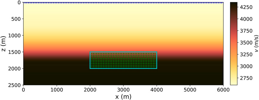
FIGURE 1. The 2-D P-wave velocity model considered for the tests. The cyan rectangular box shows the zone of interest with expected seismicity. Green dots represent 451 source positions used for training. Blue triangles on the top of the model denote 121 seismic stations. The model is taken from Hao et al. (2020).

The architecture of the feed-forward neural network is shown in Figure 2. The network consists of three hidden layers with 40 neurons (M = 40 in Figure 2) in each layer (Hao et al., 2020). The number of neurons in the input layer equals the number of stations (N = 121 in Figure 2), while two neurons in the output layer correspond to the two coordinate axes (D = 2 in Figure 2). The activation function for the hidden layer is the rectified linear unit (ReLU), a piecewise linear function, while the final layer has the linear activation function. ReLU is the default activation function for modern deep learning networks (e.g., Glorot et al. (2011)). The source code showing implementation of the described neural network model in Python is available in the Supplemental Material.

FIGURE 2

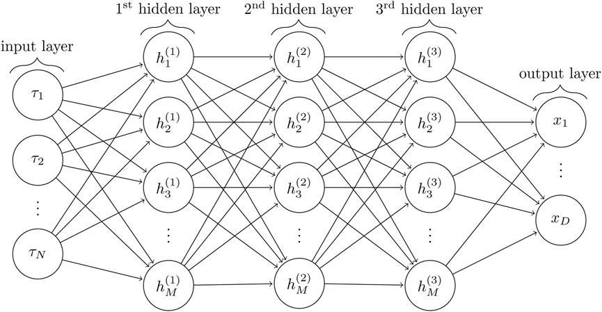
FIGURE 2. Network graph for a 3-layer perceptron with N input units and D output units, where N is a number of seismic stations with picked wave arrivals and D is a number of spatial dimensions. Each hidden layer contains M hidden units.

To train the network, we use synthetic data generated for a set of artificial sources placed on a regular grid in the zone of interest (the green dots and the rectangular box in Figure 1). Having trained the network on these sources, we test the method by feeding synthetic arrival times from 100 test sources randomly placed in the zone of interest. The traveltimes are calculated by the fast sweeping method (FSM, Zhao (2005)) at various station positions on the surface.

Following Hao et al. (2020), we present a systematic study of the different factors affecting the accuracy of the location with the ANN method. We used 1000 epochs to train the ANN in each numerical test, whereas the number of stations and the number of training grid points during these tests were varied (see Table 1). The result show that the accuracy of the located events slightly decreases with the number of training sources while training time is still very short.

TABLE 1

TABLE 1. Training time and standard deviation of location errors for different number of training sources and stations.

3.1 Effect of noise in test data

To measure the sensitivity of the ANN to potential errors in picking P-wave arrival times, we test the network by feeding in traveltimes (of test events) contaminated by Gaussian noise. We train the network using traveltime data from 451 training sources located inside the rectangular box shown in Figure 1 and spaced at an interval of 50 m along both x and z axes. The times of wave arrivals are modelled at the 121 stations on the surface (see Figure 1). Assuming no systematic bias in picking, we consider that picking errors result from random errors (noise). We consider two noise levels by adding to the arrival times a random Gaussian noise with zero mean (μ) and standard deviations (σ) of 10 ms and 20 ms.

Figure 3 shows examples of arrival times of a single test event after subtracting the mean value (see Eq. 2), contaminated with Gaussian noise of two levels, corresponding to σ = 10 ms (Figure 3A) and σ = 20 ms (Figure 3B). Figures 4A,B show distribution of location error in x and z coordinates of the source locations for the two noise levels (true locations were subtracted from predicted). We observe that location errors increase as the noise in the arrival times increases. However, even for higher noise contamination in time picks, the maximum location error does not exceed 100 m. Generally the error distributions fit to the Gaussian as seen from the black curves in Figures 4A,B. Parameters of the resulting fitting distribution in each case are shown in the legends of Figures 4A,B.

FIGURE 3

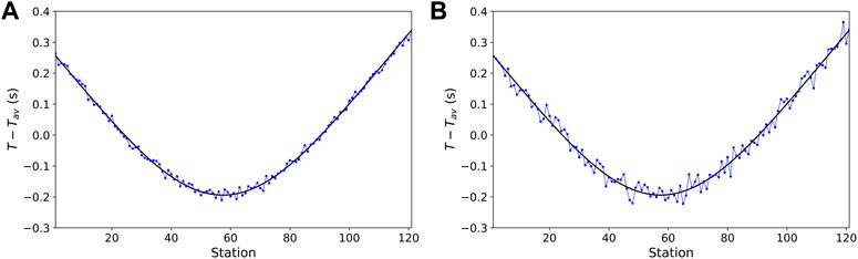
FIGURE 3. Illustration of synthetic arrival times for a test event after subtracting their mean (black curves). The arrival times contaminated with noise are shown with blue dots. (A) Arrival times contaminated with zero-mean Gaussian noise with noise level σ =10 ms. (B) Arrival times contaminated with zero-mean Gaussian noise with noise level σ =20 ms.

FIGURE 4

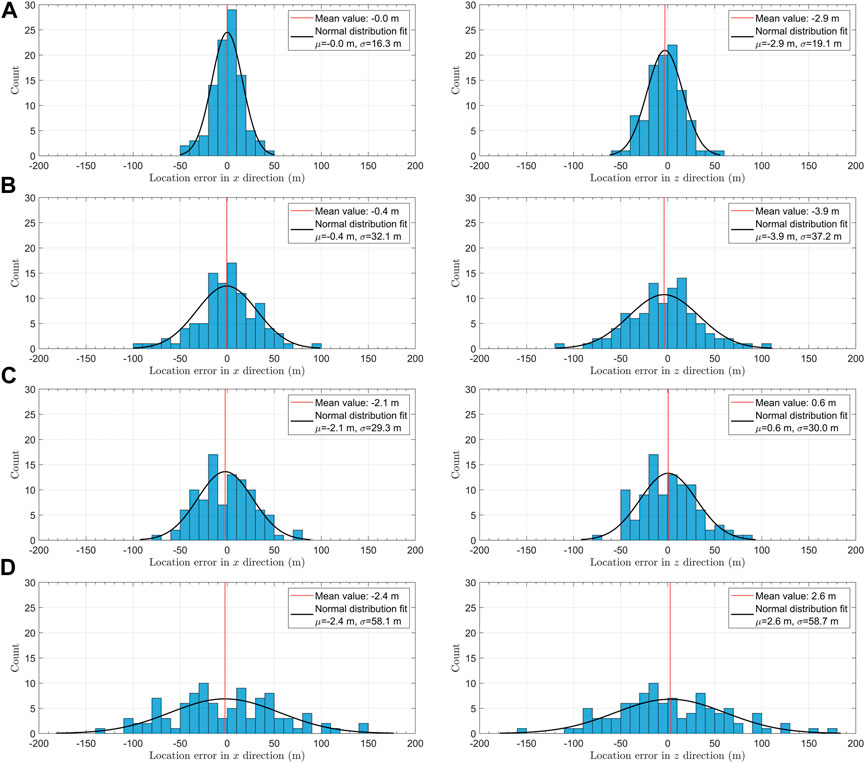
FIGURE 4. Location errors in x and z directions for 100 test sources with arrival times measured on 121 equispaced stations (A and B) and 31 equispaced stations (C and D), and contaminated by noise with Gaussian distribution and σ =10 ms (A and C) and σ =20 ms (B and D).

3.2 Effect of the number of stations

Next, we study the effect of the number of stations (receivers) on location errors. The tested model is the same as in Figure 1, but the number of stations is reduced to 31 stations spaced at an interval of 200 m. Figure 4C shows location errors for test data from the same 100 sources with a Gaussian noise corresponding to σ = 10 ms. By comparing Figures 4A,C, we observe considerable reduction in location accuracy when the number of stations is reduced. We observe that the standard deviation of location errors considerably increases (almost twice).

Figure 4D shows location error histograms for the arrival time noise level of σ = 20 ms. We observe, similar to the previous case, that increased noise worsens the location accuracy (in agreement with Hao et al., 2020). However, when the number of stations in the monitoring array is reduced, the reduction in accuracy is greater, indicating increased sensitivity to noise. Since the monitoring array is horizontal and we are using P-wave traveltimes, the vertical location is less constrained, and therefore the vertical location errors increase more than the horizontal errors. However, even in the worst considered scenario, the maximum location error observed is around 150 m, which is about three steps of the training grid (50 m).

3.3 Effect of the number of training sources

Finally, we study the effect of the number of sources used to train the network. Table 1 shows the training times and standard deviations of x and z location errors for the neural network trained using 451, 126, and 27 sources, corresponding to regular intervals of 50 m, 100 m, and 250 m, and for different station distributions: with 31 and 121 stations. The test data in all cases were contaminated by Gaussian noise with σ = 10 ms. Computations were performed on a laptop with NVIDIA GeForce MX150 graphics card.

It is obvious that the training time reduces as the number of training sources decreases, but the reduction in accuracy is significant. The training time is also slightly less if fewer stations are used. This observation suggests using a higher number of sources will improve the location accuracy. It is worth noting that a smaller training grid but a denser station array gives higher horizontal accuracy than a larger training grid but a coarser station array. This is not always true for vertical accuracy, which seems to be more sensitive to the number of training nodes.

4 Real data examples

To test the ANN method on real data, we apply the methodology to the field microseismic monitoring dataset gathered on the Woodford shale reservoir (Figure 5) in Oklahoma, United States.

FIGURE 5

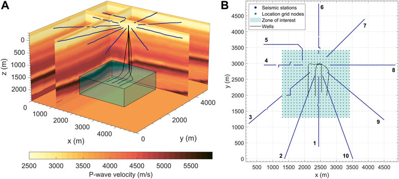
FIGURE 5. Microseismic monitoring setting at the Woodford shale reservoir in Oklahoma, United States: (A) P-wave velocity model and (B) data acquisition geometry. (A) 3-D view of the P-wave velocity model. The colorbar displays the color-coded P-wave velocities in m/s. The blue dots on the surface are seismic stations. The cyan rectangular box shows the zone of interest around lateral parts of the four wells (black lines). The zone ranges from 1303.02 m (4275 ft) to 3406.14 m (11175 ft) along the x (easting) and y (northing) axes, and from 1546.86 m (5075 ft) to 2278.38 m (7475 ft) along the z (depth) axis. (B) Map view of the data acquisition geometry: the star-like seismic station array with 10 arms (numbers) and 911 stations (blue dots), the 24 x 24 x 9 location grid with 5184 nodes (green squares show only 576 upper grid nodes), distributed over the zone of interest (cyan square), resulting in the grid spacing of 91.44 m (300 ft).

4.1 Real seismic monitoring setting

Figure 5 show the 3-D inhomogeneous isotropic P-wave velocity model (Figure 5A) and the microseismic data acquisition geometry (Figure 5B). The original grid spacing of the velocity model in x-, y- and z-directions is uniform and equal to 22.86 m (75 ft). Geophones recording vertical displacement component are distributed in the form of a star-like array with 10 arms (Figure 5B), comprising 911 seismic stations in total.

The same microseismic monitoring setting and dataset was used by Anikiev et al. (2014) to benchmark the diffraction stacking location technique (see also Anikiev (2015)). The velocity model was derived from the processing of active source data or sonic logs and calibrated with sources at known positions (Anikiev et al., 2014). In this paper we benchmark the ANN methodology by comparing it with the traveltime maximum likelihood (TML) method (Eisner et al., 2010), following Anikiev et al. (2014).

The TML algorithm minimizes the misfit between manually picked arrival times and synthetic traveltimes calculated for a reference velocity model (Anikiev et al., 2021). Hypocenter locations then are obtained from a resulting probability density function. Therefore, the TML: (i) uses the same input data as the ANN and (ii) is also based on residual minimization (Anikiev et al., 2021). This makes both ANN and TML methods suitable for comparison with the TML method used as a benchmark.

4.2 Preliminary synthetic ANN test for the real monitoring setting

Similar to a 2-D synthetic numerical study, for the 3-D case study we also design the feed-forward artificial neural network with three hidden layers (see Figure 2). Provided that synthetic data do not have gaps, the input layer consists of 911 neurons (N = 911 in Figure 2), each of which represents an arrival time deviation (Eq. 2) at the appropriate station. Each of the three hidden layers has 250 neurons (M = 250 in Figure 2). The array of seismic stations in this real example is larger than the one used in the 2-D study, leading to a larger amount of neurons in the hidden layers. The output layer now consists of 3 neurons (D = 3 in Figure 2), which represent the predicted x-, y- and z-coordinates of the event hypocenter.

Location grid for TML is represented by an array of 5184 grid nodes consisting of 24 × 24 nodes in 9 vertical planes (Figure 5). The grid nodes are regularly distributed over the zone of interest (cyan rectangular block in Figure 5A) around lateral parts of the four wells (Figure 5B), so that the resulting grid spacing of the location grid is 91.44 m (300 ft) in all directions. For consistency, the same grid was used to produce the training data, i.e. 5184 training sources were placed to the positions of the location grid nodes, forming a training grid (see also Anikiev et al., 2021).

For each training source, we applied the 3-D factored FSM algorithm (Fomel et al., 2009) to obtain the synthetic traveltimes at all the stations. The factored FSM significantly reduces the location error, especially in depth, due to much higher accuracy of computed traveltimes at far offsets (Alexandrov et al., 2021). The computed traveltimes, after removing the mean (Eq. 2) and scaling (Eq. 3), are used as an input for the ANN, which is then trained until its output matches the coordinates of the training sources by minimizing the loss function 4.

In order to evaluate the performance of the ANN by using the synthetic data, we randomly generated 100 test sources inside the zone of interest (Figure 5) and computed the corresponding traveltimes from these sources to the seismic stations with the factored FSM using the known velocity model. Figure 6 shows the error distributions of the predicted source coordinates (true locations were subtracted from predicted). The maximum errors in the x- and y-coordinates do not exceed 10 m, and the maximum error in the z-coordinate is less than 20 m, which is close to the grid spacing interval of the velocity model (22.86 m) and much smaller than the training grid spacing (91.44 m). The mean values of the observed error distributions are close to zero. The forms of these distributions are similar to Gaussian, implying that the locations should be correct as long as the input arrival times are correct.

FIGURE 6

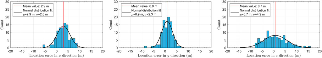
FIGURE 6. Location errors in three directions: x (left), y (middle) and z (right) for 100 test sources (without noise). Black curve in each panel show result of Gaussian distribution fit, corresponding parameters are listed in the panel legend.

4.3 Benchmarking on real data

For benchmarking we selected 75 independent seismic events strong enough to be picked on majority of stations without stacking. Figure 7 shows deviation times (see Eq. 2) obtained from manual P-wave arrival time picking for all 75 events on 911 stations. White gaps correspond to the stations for which the picking was not possible or not reliable (Anikiev et al., 2021). The seismic events are sorted by the number of missing arrival time picks. This number varies from 41 for the best picked event (event 1, Figure 7) to 503 for the worst picked event (event 75, Figure 7). Figure 7 shows that even the most distinct event (event 1) has clear P-wave arrivals only on 870 stations out of 911.

FIGURE 7

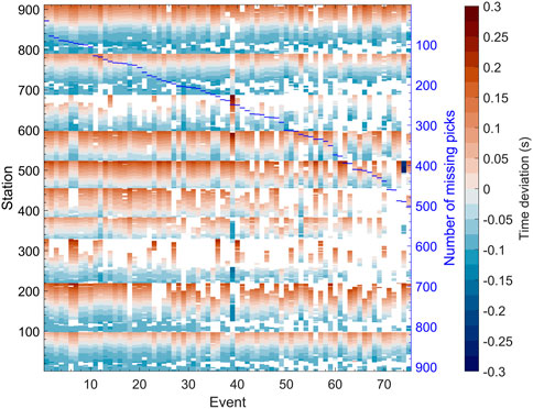
FIGURE 7. Deviation times obtained from manual P-wave arrival time picking for 75 real microseismic events recorded with 911 seismic stations. Blue horizontal dashes show number of missing (out of 911) time picks (right axis) for each event.

Event 39 has different picking pattern due to an unusual distinctive moveout and apex point of the traveltime curve, indicating a unique epicenter position. Event 74 (second last) was incorrectly picked at several stations at the far offset of the 6-th arm (see Figure 5B). These picking errors result in the set of big negative deviations of arrival time (see Figure 7). We kept this incorrectly picked event to compare the sensitivity of the two methods to a real case scenario where either a human or a picking algorithm wrongly identifies the P-wave arrival. We observe that the ANN algorithm results in a similar location anomaly as the TML. Classical traveltime-based location methods like TML are flexible to missing data. In contrast to that, data gaps introduce a serious fundamental complexity for feed-forward ANNs, which require regular input.

As a proof of concept for real data, following Anikiev et al. (2021), we first tested a “brute-force” approach by training the ANN from scratch for each real event separately, taking into account only stations with available time picks. This means that we re-trained the neural network for each picked event using only the stations with available picks. In the data application of Anikiev et al. (2021) a fixed number of training epochs (4000) and an initial learning rate of 10^–4 were used. This could result in an overfitting, especially when the validation set (100 random sources) has a similar distribution to the training data. Overfitting is a common problem in ML which occurs when the ANN fits the training data too well. In order to avoid overfitting we follow a different approach. We first split the training data and use 15% of initial dataset for validation and then implemented early stopping (e.g., Chollet, 2015), i.e. tracking the validation loss and stopping the training before overfitting occurs. This has also reduced the overall time cost of the training. We used a patience parameter of 100 as a stopping criteria in each case. The patience parameter is a number of epochs with no improvement after which training will be stopped (see Keras API documentation (Chollet, 2015). Moreover, we set a loss function value threshold of 391.9 m² as an additional criterion. If loss function goes lower than this threshold, the training stops. The threshold value was estimated from the velocity model grid step of 22.86 m: 3 × (22.86/2)² = 391.9. This means that if the misfit is corresponding to one-half of the velocity model grid step (used also for traveltime computation), the training already reaches the reasonable accuracy level, although some other multiples of the grid step might be also acceptable. Application of these two criteria provides the compromise between the accuracy and computation time of training with its numerical stability and helps to avoid over-fitting, thus making the training flexible.

Figure 8 shows comparison of the TML locations (blue circles) with the ANN locations (orange circles) for all 75 events. To produce this result for each event, we performed re-training of the ANN from scratch. As seen from Table 2, the number of epochs until stopping varied from 674 to 1943 with an average of about 1214. Event 74, which was picked with several errors, is located by the ANN method at an extremely large depth of around 4500 m, outside of the training grid (green dots in Figure 8), whereas the TML locates it close to the lower bound of the grid. This indicates that the ANN is more sensitive to data with large uncertainty (outliers, e. g, false positive detections) than the TML. Such deviations can be used in quality control as indicators of input data errors. Location misfit for the event 74 in lateral direction is smaller, so the true epicenter is expected to be to the north from the wells. Event 39, which has the aforementioned dissimilar arrival time pattern (Figure 7), is predictably located by both methods to the south-southwest from the wells and the cluster of the remaining events.

FIGURE 8

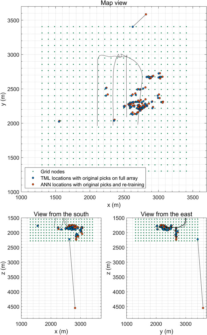
FIGURE 8. Comparison of TML locations (blue circles) with ANN locations (orange circles) obtained with re-training for all 75 events: map view (top panel), view from the south (left bottom panel), view from the east (right bottom panel). Two locations for the same event are connected with a black line. Green dots represent the grid nodes for the TML, also used as training sources for the ANN. Wells are shown with black lines.

TABLE 2

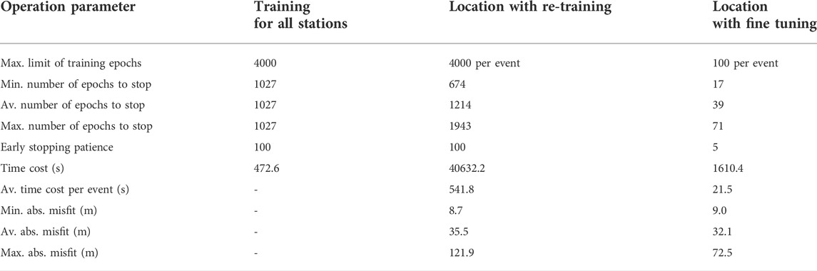
TABLE 2. Computation time costs for the ANN training and location of 75 events, and location misfits when compared with the TML.

If we take a closer look into the locations of the 74 reliably picked events (excluding the event 74), as displayed by Figure 9, we see that horizontal misfit between the locations by TML and ANN does not exceed the spacing of the location (training) grid even for the distant event 39 (southwestern corner on the map view in Figure 9). Vertical misfit is generally larger but is comparable to the grid spacing as well (in agreement with Anikiev et al., 2021).

FIGURE 9

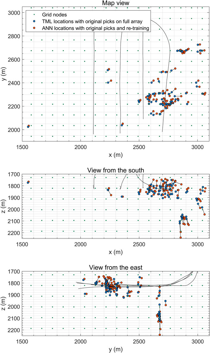
FIGURE 9. Comparison TML locations (blue circles) with ANN locations (orange circles) obtained with re-training for 74 reliably picked events: map view (top panel), view from the south (middle panel), view from the east (bottom panel). Two locations for the same event are connected with a black line. Green dots represent the grid nodes for the TML, also used as training sources for the ANN. Wells are shown with black lines.

To avoid the time-consuming re-training from beginning, we propose to use fine tuning (transfer learning in Anikiev et al. (2021), i.e., make use of the weights of a pre-trained network to speed up adaptation to the new input pattern. Technically, fine tuning consists of unfreezing the initially trained model and further additional training on the new data with a lower learning rate. The neural network is first pre-trained on the complete array of stations with the same stopping criteria mentioned before. The trained weights and biases are then transferred into the corresponding layer of a new neural network that is designed for each event with its own input layer dimension according to the pattern of available P-wave arrival time picks. Finally, this newly set network is shortly trained (fine-tuned) with a patience of 5 and the last used learning rate taken from the pre-training.

Figure 10 shows the TML locations of the same 74 reliably picked events compared to the ANN location obtained with fine tuning. We observe that the locations obtained using fine tuning are similar to those obtained with the entirely re-trained neural network, but they are achieved much faster. The average misfit of locations obtained with fine tuning with TML locations is lower (see Table 2). At the same time fine tuning significantly reduces the amount of required training epochs and time cost. The average time cost with fine tuning is roughly 25 times lower. The pre-training stopped at 1027 epochs, which took less than 8 min (Table 2), while an average of 39 epochs in terms of fine tuning per each event provide sufficient accuracy in tens of seconds (Table 2, Figure 10). All computations were performed on the same machine as in the synthetic data case.

FIGURE 10

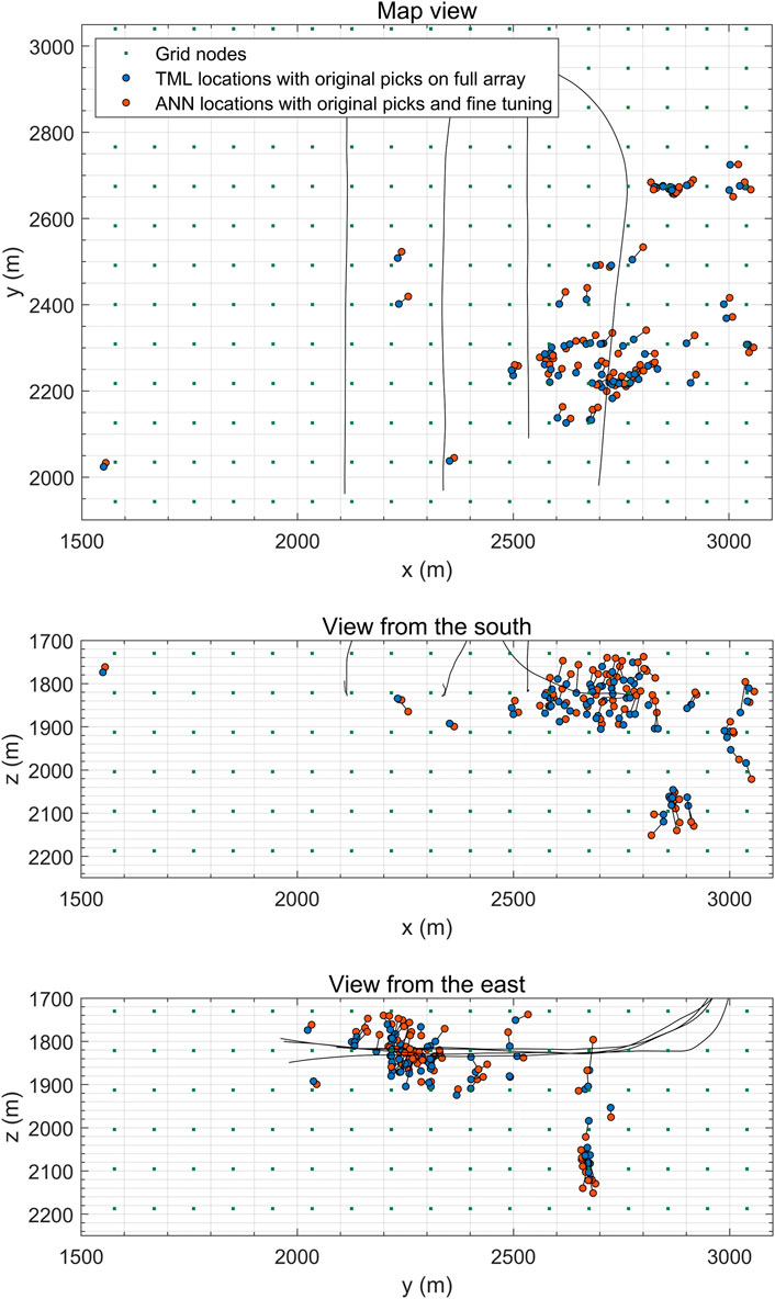
FIGURE 10. Comparison of TML locations (blue circles) with ANN locations (orange circles) obtained with fine tuning for 74 reliably picked events: map view (top panel), view from the south (middle panel), view from the east (bottom panel). Two locations for the same event are connected with a black line. Green dots represent the grid nodes for the TML, also used as training sources for the ANN. Wells are shown with black lines.

Figure 11, Figure 12 show histograms of misfit in x-, y- and z-directions together with absolute misfits for ANN with re-training and ANN with fine tuning, respectively. The lateral misfits in case of ANN with fine tuning do not exceed 40 m, which is twice as less than the training grid spacing of 91.44 m (Figure 12). The vertical misfits are predictably larger, especially in case of ANN with re-training, where it reaches 120 m (Figure 11). The standard deviations of the misfit distributions in lateral direction are similar for both results. In contrast, the standard deviation of the vertical misfit is smaller for locations in Figure 12 obtained with fine tuning. The distribution of the absolute misfits (square root of the sum of squared misfits in x-, y- and z-directions) in both cases fits well to the non-central χ distribution with 3 degrees of freedom. The latter is mathematically consistent with the distribution of the absolute value (square root of sum of squares) of the three independent normally distributed quantities with non-zero mean (e.g., Bhattacharya and Burman (2016). The distribution is described by the non-centrality parameter, reflecting the characteristic difference between the two results. Statistical distributions for both cases (ANN with re-training and with fine tuning) can be described with non-centrality parameter much smaller than the training grid step. The maximum absolute misfit for fine tuning (Figure 11) is less than 80 m, so it does not exceed the training grid step, whereas for ANN with re-training it exceeds it with values over 120 m.

FIGURE 11

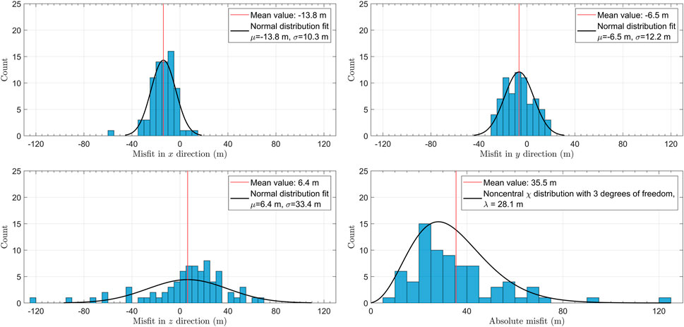
FIGURE 11. Histograms of misfits between TML locations and ANN locations obtained with re-training for 74 reliably picked events. Black curve in each panel shows the result of distribution fit with the corresponding parameters listed in the panel legend.

FIGURE 12

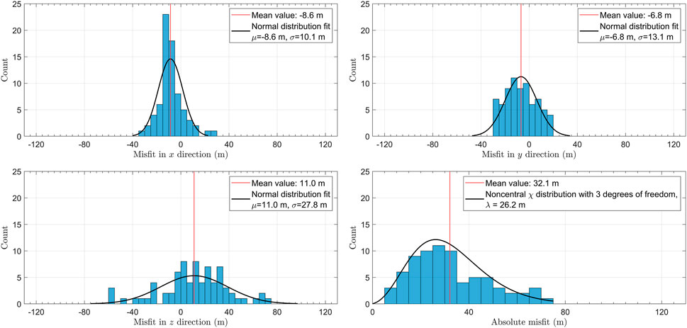
FIGURE 12. Histograms of misfits between TML locations and ANN locations obtained with fine tuning for 74 reliably picked events. Black curve in each panel shows the result of distribution fit with the corresponding parameters listed in the panel legend.

Comparison of Figure 9 with Figure 10 and Figure 11 with Figure 12 shows that the proposed ANN methodology extended with fine tuning provides sufficient location accuracy without time consuming computations, as illustrated by Table 2.

5 Discussion

In the proposed ANN method the neural network is trained only with synthetic data, i.e., no existing seismic data are needed (although the method does not exclude the ability to use existing catalog locations), and so the training can be done before the monitoring starts. However, if enough seismic events in the area are observed previously, it can be trained using P-wave arrivals and locations of these real events. Obviously, the accuracy of the network trained with real events depends on number of events and spatial distribution of their locations. Training with synthetic data is more time consuming and computationally expensive but the accuracy of resulting ANN locations is higher. The time needed to locate a single event stays the same once the network is pre-trained, no matter whether the training is done with synthetic or real data.

A typical workflow for deployment of the proposed method for microseismic monitoring is represented in Figure 13. The most time consuming parts: computation of the traveltime lookup table and training of the ANN are performed before the monitoring starts. Real-time detection stage can also be implemented with the help of ML (out of the scope of this paper). The essential part of detection stage is to provide the P-wave arrival times for a certain subset of stations (picking depends on the quality of the record and often cannot be done reliably on all stations). Real-time location then requires inexpensive fine tuning of the initially trained NN for the provided set of stations. The fine-tuned network model is stored and re-used for further events with the same subset of stations, thus reducing the processing time. We suggest to use the 3-layer perceptron architecture of the NN explained by Figure 2, where M = 250 is optimal for number of recording seismic stations N around 1000.

FIGURE 13

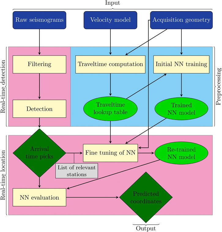
FIGURE 13. The flowchart showing a typical implementation of ANN-based location in real-time microseismic monitoring setting. Time consuming blocks in the blue zone belong to a pre-processing stage performed prior to the monitoring, while blocks in the reddish zones are in real time. Blue blocks represent input data, yellow blocks correspond to processes, green ellipses show intermediate products and deep-green diamonds show the output: arrival time picks and predicted hypocenter coordinates. Gray block denotes that fine tuning requires only the list of relevant stations, arrival time picks from raw seismograms are used for NN evaluation only.

In real-time monitoring applications, time to deliver the source locations is important. We have shown that combining fine-tuning with early stopping and additional loss function threshold gives a compromise between the location accuracy and computation time required for additional training. The fine tuning step is done in seconds on a mobile mid-range GPU and won’t be a bottleneck in real-time implementations on more performant GPU systems.

As we show on synthetic examples, the developed ANN method suffers from the same known limitations as all the other location methods when monitoring with surface array. The average location uncertainty in vertical direction is typically higher than in horizontal directions when only P-wave arrival times are input. If data quality allows, methods can be usually extended with S-wave arrivals and location accuracy improves. Location quality decreases with higher uncertainty of picks (related to SNR of arrivals in real data) and with coarser training grid. However, in our case, the latter can be easily eliminated as the ANN can be pre-trained with synthetic events in an arbitrarily dense training grid.

Location uncertainty estimates are highly dependent on the accuracy of the velocity model, which is always different. We have tested the accuracy of location based on synthetic tests and provided estimates of the standard deviation in each case. We consider this to be a fair representation of the potential location error. Integration of the dedicated uncertainty estimates into the ML prediction is a more sophisticated task which is out of the scope of the present manuscript. It is certainly one of the directions for further advanced studies.

In real data, signal-to-noise ratio varies for each event and consequently number of input stations with available picks changes, leading to gaps in the input data. In order to solve this problem we initially considered several options.

First, one can use interpolation of the data at the stations with missing time picks. Interpolation methods for uniform grids are not applicable in this case, as the stations are usually distributed irregularly. The kriging method (Stein, 1999) models the interpolated data through a Gaussian process governed by prior covariances, and it is applicable to irregular grids. The kriging algorithm performs well for small local gaps, e.g., when few stations with missing picks are surrounded by the stations with available time arrivals. However, it can introduce a significant bias in the case when the missing picks occur on the stations at the edge of the network or along a certain direction due to the radiation pattern defined by the source mechanism of an earthquake. Such a situation is typical when using star-like geometries (Anikiev et al., 2014; Staněk et al., 2015). Besides, any interpolation method is likely to introduce a non-physical distortion to the set of traveltimes in the case of a coarse network of stations.

The benchmark comparison with the TML method shows that the proposed location algorithm is as good as any other arrival time based location technique. It provides good location if the velocity model is good and arrival times are correctly picked. Velocity model errors are perhaps the most significant source of location biases in both surface and downhole monitoring (Eisner et al., 2010). Very much the same as for any other arrival time based method (e.g., for the mentioned TML method), the errors in velocity model in the proposed ANN approach influence only the traveltime computation. Therefore, we consider the accuracy of the velocity model to be a more general problem that has already been covered in literature. For instance, Eisner et al. (2009) presented an extensive study of the effect of errors in the velocity model on locations derived from arrival time picks by simulating uncertainties for frequently used borehole and surface acquisition receiver geometries and assuming a homogeneous medium.

Another option for benchmarking would be to use any other conventional location method to calculate the traveltimes based on the estimated location. This means that prior to the prediction of location by the ANN, the real traveltimes are “regularized” using the modeled ones. For such an approach, the TML methodology suits the best, as it is based on the maximum likelihood of traveltimes, which is consistent with the chosen cost function in our algorithm. However, there is an obvious disadvantage of this approach–for each event, it requires an additional step of location, therefore making the ANN-based location computationally less attractive.

Finally, in order to be independent of the missing data, one could pre-train many ANNs for different sets of available stations. Every possible combination of stations requires 2^N trainings with N being a number of seismic stations. It possible for very small N and is out of question for large N. Alternatively, we may consider training only for a certain set of “backbone” stations where all events are picked, and throwing away all other picks on the remaining stations.

After testing the aforementioned methods, we decided to use fine tuning to overcome the issue of missing picks. Fine tuning is an effective method taking advantage of weights of ANN obtained after training with full array of stations acquiring data. With a limited number of epochs, we are able to quickly train ANN specific for each individual event picked on a specific subset of stations. The other methods seem not to be as robust and accurate as the fine-tuning approach.

A ML location method that is flexible to the number of seismic stations was proposed by van den Ende and Ampuero (2020), who developed a graph neural network (GNN) approach which is also invariant to the order in which the stations are arranged. First, authors suggest to analyze the waveforms on each station using a CNN which extracts certain features, and then the location of stations is appended to form a feature vector that serves as an input for the second multilayer perceptron (MLP) component. After performing the operation on every station, the results are combined into a graph feature vector. So far we have considered to adapt this approach for traveltime-based location, where the selected feature at each station is the picked arrival time. GNN might result in potential improvement, but the challenge is in enforcing the feature to be the arrival time.

6 Conclusion

A machine learning methodology proposed earlier was extended in this paper into a practical technique capable of locating real microseismic events in a typical microseismic monitoring setting. This extension represents a non-trivial task which was not anticipated earlier.

The location method is based on P-wave arrival picks input and artificial neural network trained on a set of known locations. Its main advantage is a possibility to train the system only with synthetic data, i.e., no existing seismic data are needed before its application. Therefore, the training can be successfully done even in areas where any prior seismicity has not been observed, and it can be done in advance, before the actual seismic monitoring starts.

The training dataset is computed with known velocity model, monitoring array, and a set grid of training locations in the subsurface. The ANN must be trained with the same (sub-)set of stations as the data of real event are from. However, in reality, a subset of stations with available picks for each event changes due to various reasons (variable SNR, missing stations, etc.). To overcome this problem, we use fine tuning: the weights of ANN obtained after training using full array of seismic stations are used as initial values and a new ANN can be quickly trained for each individual event picked on a specific subset of stations. In order to prevent overfitting we further investigated the use of early stopping by reserving part of the training data for validation and tracking the validation loss.

The extended methodology was tested on 2D and 3D synthetic examples that allowed us to determine optimal neural network parameters and estimate location errors. We showed that accuracy of resulting locations increases with density of training location grid, number of available seismic stations and quality of input data, which is in agreement with the behavior of classical location methods. The ANN method was benchmarked against a commonly used TML method on a real dataset acquired during hydraulic fracturing. We demonstrated that locations from both methods are comparable and the location misfit is similar to the training grid spacing when a reliable velocity model is used. However, the ANN-based location is less sensitive to gridding, more sensitive to data outliers, and implies simple and straight-forward training. Use of the early stopping criterion presented in this study helped to significantly reduce the computation time both for initial training using the full set of seismic stations and for the fine-tuning training step.

Analysis of real data application results show that the proposed approach is efficient and can be applied during real-time monitoring when combined with reliable automatic event detection and arrival time picking algorithms. We proposed a workflow for implementation of the method in the real-time monitoring setting.

Data availability statement

The data analyzed in this study is subject to the following licenses/restrictions: The data underlying this article were provided by Newfield Exploration Mid Continent Inc. and MicroSeismic, Inc. by permission. Data will be shared on reasonable request to the corresponding author with permission of MicroSeismic, Inc. The source code showing implementation of the described neural network model in Python is available in the Supplemental Material. Other source codes will be shared on reasonable request to the corresponding author. Requests to access these datasets should be directed to denis.anikiev@gfz-potsdam.de.

Author contributions

This study was conceptualized by LE, UW and QH, with contributions from DAn and FS. The ANN model has been set up, trained and tested on synthetic data by QH with contributions from UW and DAn. FS prepared the real dataset and model with contributions by DAn. The methodology for real data processing was developed by DAn and UW with contributions from FS. The ANN model application to real data including the fine tuning approach was prepared by DAn. The artwork was prepared by DAn with contributions from QH. The results have been analysed by UW and LE with contributions by DAl, NI and QH. The final manuscript has been written by DAn and UW, with contributions by LE, FS, DAl, NI and QH.

Funding

The research is funded by the Helmholtz Centre Potsdam–GFZ German Research Centre for Geosciences (Germany), King Fahd University of Petroleum (Saudi Arabia) and Minerals and Seismik s. r.o (Czech Republic). Publication costs are supported within the funding programme “Open Access Publikationskosten” Deutsche Forschungsgemeinschaft (DFG, German Research Foundation) - Project Number 491075472.

Acknowledgments

The authors thank the College of Petroleum Engineering and Geosciences at KFUPM and Basin Modelling Section at GFZ for support. The Woodford field dataset and model is courtesy of Newfield Exploration Mid Continent Inc. and MicroSeismic, Inc. We are grateful to all the reviewers for their valuable and constructive comments which helped us to improve the manuscript.

Conflict of interest

Authors DAl and LE were employed by the company Seismik s.r.o.

The remaining authors declare that the research was conducted in the absence of any commercial or financial relationships that could be construed as a potential conflict of interest.

Publisher’s note

All claims expressed in this article are solely those of the authors and do not necessarily represent those of their affiliated organizations, or those of the publisher, the editors and the reviewers. Any product that may be evaluated in this article, or claim that may be made by its manufacturer, is not guaranteed or endorsed by the publisher.

Supplementary material

The Supplementary Material for this article can be found online at: https://www.frontiersin.org/articles/10.3389/feart.2022.1046258/full#supplementary-material

References

Abadi, M., Agarwal, A., Barham, P., Brevdo, E., Chen, Z., Citro, C., et al. (2015). TensorFlow: Large-scale machine learning on heterogeneous systems. Available at: http://download.tensorflow.org/paper/whitepaper2015.pdf.

Google Scholar

Alexandrov, D., bin Waheed, U., and Eisner, L. (2021). Microseismic location error due to eikonal traveltime calculation. Appl. Sci. 11, 982. doi:10.3390/app11030982

CrossRef Full Text | Google Scholar

Anikiev, D., bin Waheed, U., Staněk, F., Alexandrov, D., and Eisner, L. (2021). “Microseismic event location using artificial neural networks,” in First international meeting for applied geoscience & energy expanded abstracts (Texas, United States: Society of Exploration Geophysicists), 1661–1665. doi:10.1190/segam2021-3582729.1

CrossRef Full Text | Google Scholar

Anikiev, D. (2015). “Location and source mechanism determination of microseismic events,” Ph.D. thesis (St. Petersburg, Russia: St. Petersburg State University).

Google Scholar

Anikiev, D., Valenta, J., Staněk, F., and Eisner, L. (2014). Joint location and source mechanism inversion of microseismic events: Benchmarking on seismicity induced by hydraulic fracturing. Geophys. J. Int. 198, 249–258. doi:10.1093/gji/ggu126

CrossRef Full Text | Google Scholar

Bhandarkar, T., K, V., Satish, N., Sridhar, S., Sivakumar, R., and Ghosh, S. (2019). Earthquake trend prediction using long short-term memory RNN. Int. J. Electr. Comput. Eng. (IJECE) 9, 1304. doi:10.11591/ijece.v9i2.pp1304-1312

CrossRef Full Text | Google Scholar

Bhattacharya, P. K., and Burman, P. (2016). Theory and methods of statistics. Massachusetts, United States: Academic Press.

Google Scholar

Birnie, C., and Alkhalifah, T. (2022). “Leveraging domain adaptation for efficient seismic denoising,” in Energy in Data Conference, Austin, Texas, 20–23 February 2022, 11–15. Energy in Data. doi:10.7462/eid2022-04.1

CrossRef Full Text | Google Scholar

Chollet, F. (2015). Keras. Available at: https://keras.io/.

Google Scholar

Cremen, G., and Galasso, C. (2020). Earthquake early warning: Recent advances and perspectives. Earth-Science Rev. 205, 103184. doi:10.1016/j.earscirev.2020.103184

CrossRef Full Text | Google Scholar

Dramsch, J. S. (2020). 70 years of machine learning in geoscience in review. Adv. Geophys. 61, 1–55. doi:10.1016/bs.agph.2020.08.002

CrossRef Full Text | Google Scholar

Duncan, P. M., and Eisner, L. (2010). Reservoir characterization using surface microseismic monitoring. Geophysics 75, 75A139–75A146. doi:10.1190/1.3467760

CrossRef Full Text | Google Scholar

Eisner, L., Duncan, P. M., Heigl, W. M., and Keller, W. R. (2009). Uncertainties in passive seismic monitoring. Lead. Edge 28, 648–655. doi:10.1190/1.3148403

CrossRef Full Text | Google Scholar

Eisner, L., Hulsey, B. J., Duncan, P., Jurick, D., Werner, H., and Keller, W. (2010). Comparison of surface and borehole locations of induced seismicity. Geophys. Prospect. 58, 809–820. doi:10.1111/j.1365-2478.2010.00867.x

CrossRef Full Text | Google Scholar

Ellsworth, W. L. (2013). Injection-induced earthquakes. Science 341, 1225942. doi:10.1126/science.1225942

PubMed Abstract | CrossRef Full Text | Google Scholar

Fomel, S., Luo, S., and Zhao, H. (2009). Fast sweeping method for the factored eikonal equation. J. Comput. Phys. 228, 6440–6455. doi:10.1016/j.jcp.2009.05.029

CrossRef Full Text | Google Scholar

Fornasari, S. F., Pazzi, V., and Costa, G. (2022). A machine-learning approach for the reconstruction of ground-shaking fields in real time. Bull. Seismol. Soc. Am. 112, 2642–2652. doi:10.1785/0120220034

CrossRef Full Text | Google Scholar

Foulger, G. R., Wilson, M. P., Gluyas, J. G., Julian, B. R., and Davies, R. J. (2018). Global review of human-induced earthquakes. Earth-Science Rev. 178, 438–514. doi:10.1016/j.earscirev.2017.07.008

CrossRef Full Text | Google Scholar

Glorot, X., Bordes, A., and Bengio, Y. (2011). “Deep sparse rectifier neural networks,” in Proceedings of the Fourteenth International Conference on Artificial Intelligence and Statistics. Editors G. Gordon, D. Dunson, and M. Dudík (Fort Lauderdale, FL, USA: JMLR Workshop and Conference Proceedings), 315–323. 15 of Proceedings of Machine Learning Research.

Google Scholar

Hao, Q., Waheed, U., Babatunde, M., and Eisner, L. (2020). Microseismic hypocenter location using an artificial neural network. In 82nd EAGE Annual Conference & Exhibition European Association of Geoscientists & Engineers, December 8–11, 2022. 2020, 1–5. doi:10.3997/2214-4609.202010583

CrossRef Full Text | Google Scholar

Häring, M. O., Schanz, U., Ladner, F., and Dyer, B. C. (2008). Characterisation of the basel 1 enhanced geothermal system. Geothermics 37, 469–495. doi:10.1016/j.geothermics.2008.06.002

CrossRef Full Text | Google Scholar

Kingma, D. P., and Ba, J. (2014). Adam: A method for stochastic optimization. arXiv preprint arXiv:1412.6980. Availablble at: https://arxiv.org/abs/1412.6980 (Accessed Dec 22, 2014).

Google Scholar

Kong, Q., Trugman, D. T., Ross, Z. E., Bianco, M. J., Meade, B. J., and Gerstoft, P. (2019). Machine learning in seismology: Turning data into insights. Seismol. Res. Lett. 90, 3–14. doi:10.1785/0220180259

CrossRef Full Text | Google Scholar

Kriegerowski, M., Petersen, G. M., Vasyura-Bathke, H., and Ohrnberger, M. (2018). A deep convolutional neural network for localization of clustered earthquakes based on multistation full waveforms. Seismol. Res. Lett. 90, 510–516. doi:10.1785/0220180320

CrossRef Full Text | Google Scholar

Li, L., Tan, J., Schwarz, B., Staněk, F., Poiata, N., Shi, P., et al. (2020). Recent advances and challenges of waveform-based seismic location methods at multiple scales. Rev. Geophys. 58, e2019RG000667. doi:10.1029/2019rg000667

CrossRef Full Text | Google Scholar

Maxwell, S. C., Rutledge, J., Jones, R., and Fehler, M. (2010). Petroleum reservoir characterization using downhole microseismic monitoring. Geophysics 75, 75A129–75A137. doi:10.1190/1.3477966

CrossRef Full Text | Google Scholar

Mousavi, S. M., and Beroza, G. C. (2020). A machine-learning approach for earthquake magnitude estimation. Geophys. Res. Lett. 47, e2019GL085976. doi:10.1029/2019gl085976

CrossRef Full Text | Google Scholar

Mousavi, S. M., Ellsworth, W. L., Zhu, W., Chuang, L. Y., and Beroza, G. C. (2020). Earthquake transformer—An attentive deep-learning model for simultaneous earthquake detection and phase picking. Nat. Commun. 11, 3952. doi:10.1038/s41467-020-17591-w

PubMed Abstract | CrossRef Full Text | Google Scholar

Nooshiri, N., Bean, C. J., Dahm, T., Grigoli, F., Kristjánsdóttir, S., Obermann, A., et al. (2021). A multibranch, multitarget neural network for rapid point-source inversion in a microseismic environment: Examples from the hengill geothermal field, Iceland. Geophys. J. Int. 229, 999–1016. doi:10.1093/gji/ggab511

CrossRef Full Text | Google Scholar

Perol, T., Gharbi, M., and Denolle, M. (2018). Convolutional neural network for earthquake detection and location. Sci. Adv. 4, e1700578. doi:10.1126/sciadv.1700578

PubMed Abstract | CrossRef Full Text | Google Scholar

Ross, Z. E., Trugman, D. T., Hauksson, E., and Shearer, P. M. (2019). Searching for hidden earthquakes in southern California. Science 364, 767–771. doi:10.1126/science.aaw6888

PubMed Abstract | CrossRef Full Text | Google Scholar

Rutledge, J. T., and Phillips, W. S. (2003). Hydraulic stimulation of natural fractures as revealed by induced microearthquakes, Carthage Cotton Valley gas field, east Texas. Geophysics 68, 441–452. doi:10.1190/1.1567214

CrossRef Full Text | Google Scholar

Saad, O. M., Bai, M., and Chen, Y. (2021). Uncovering the microseismic signals from noisy data for high-fidelity 3D source-location imaging using deep learning. Geophysics 86, KS161–KS173. doi:10.1190/geo2021-0021.1

CrossRef Full Text | Google Scholar

Saad, O. M., and Chen, Y. (2021). Earthquake detection and P-wave arrival time picking using capsule neural network. IEEE Trans. Geosci. Remote Sens. 59, 6234–6243. doi:10.1109/tgrs.2020.3019520

CrossRef Full Text | Google Scholar

Schultz, R., Beroza, G., Ellsworth, W., and Baker, J. (2020). Risk-informed recommendations for managing hydraulic fracturing–induced seismicity via traffic light protocols. Bull. Seismol. Soc. Am. 110, 2411–2422. doi:10.1785/0120200016

CrossRef Full Text | Google Scholar

Staněk, F., Anikiev, D., Valenta, J., and Eisner, L. (2015). Semblance for microseismic event detection. Geophys. J. Int. 201, 1362–1369. doi:10.1093/gji/ggv070

CrossRef Full Text | Google Scholar

Stein, M. L. (1999). Interpolation of spatial data: Some theory for kriging. Berlin, Germany: Springer Science & Business Media.

Google Scholar

Steinberg, A., Vasyura-Bathke, H., Gaebler, P., Ohrnberger, M., and Ceranna, L. (2021). Estimation of seismic moment tensors using variational inference machine learning. J. Geophys. Res. Solid Earth 126, e2021JB022685. doi:10.1002/essoar.10507484.1

CrossRef Full Text | Google Scholar

Tous, R., Alvarado, L., Otero, B., Cruz, L., and Rojas, O. (2020). Deep neural networks for earthquake detection and source region estimation in north-central Venezuela. Bull. Seismol. Soc. Am. 110, 2519–2529. doi:10.1785/0120190172

CrossRef Full Text | Google Scholar

van den Ende, M. P. A., and Ampuero, J.-P. (2020). Automated seismic source characterization using deep graph neural networks. Geophys. Res. Lett. 47, e2020GL088690. doi:10.1029/2020gl088690

CrossRef Full Text | Google Scholar

Verdon, J. P., and Bommer, J. J. (2020). Green, yellow, red, or out of the blue? An assessment of traffic light schemes to mitigate the impact of hydraulic fracturing-induced seismicity. J. Seismol. 25, 301–326. doi:10.1007/s10950-020-09966-9

CrossRef Full Text | Google Scholar

Vinard, N. A., Drijkoningen, G. G., and Verschuur, D. J. (2021). Localizing microseismic events on field data using a u-net-based convolutional neural network trained on synthetic data. Geophysics 87, KS33–KS43. doi:10.1190/geo2020-0868.1

CrossRef Full Text | Google Scholar

Wiszniowski, J., Plesiewicz, B. M., and Trojanowski, J. (2013). Application of real time recurrent neural network for detection of small natural earthquakes in Poland. Acta Geophys. 62, 469–485. doi:10.2478/s11600-013-0140-2

CrossRef Full Text | Google Scholar

Yu, S., and Ma, J. (2021). Deep learning for geophysics: Current and future trends. Rev. Geophys. 59, e2021RG000742. doi:10.1029/2021rg000742

CrossRef Full Text | Google Scholar

Zhang, X., Zhang, M., and Tian, X. (2021). Real-time earthquake early warning with deep learning: Application to the 2016 m 6.0 central apennines, Italy earthquake. Geophys. Res. Lett. 48, 2020GL089394. doi:10.1029/2020gl089394

CrossRef Full Text | Google Scholar

Zhao, H. (2005). A fast sweeping method for eikonal equations. Math. Comput. 74, 603–627. doi:10.1090/s0025-5718-04-01678-3

CrossRef Full Text | Google Scholar

Zhu, W., and Beroza, G. C. (2018). PhaseNet: A deep-neural-network-based seismic arrival-time picking method. Geophys. J. Int. 216, 261–273. doi:10.1093/gji/ggy423

CrossRef Full Text | Google Scholar