On the Relation Between Anomalous Clouds and Earthquakes in Italian Land

Introduction

Clouds are very common in the atmosphere, and they are always considered to be related to weather change. In 1997 Russian scientist Morozova (1997) reported some unusual linear clouds above land fracture regions. This was the first report about cloud anomaly possibly related to active fault systems. Shou (1999) reported some unusual clouds which looked like they emitted from a point source 5 days prior to the 26 December 2003, M6.6 Bam, Iran, earthquake. Guo and Wang (2008) studied M6.0 and M6.4 Iran strong earthquakes and found that some linear clouds appeared about 2 months before these earthquakes. Wu et al. (2009) reported two linear clouds which pointed to the epicenter prior to the 12 May 2008, M7.9 Wenchuan earthquake of China. Guo and Yang (2013) observed an anomalous linear cloud over Italy on April 23, 2012, and predicted that an M5.5–M6.0 earthquake would hit Italy in the next month. An M6.1 earthquake hit north Italy on 20 May 2012, and verified this prediction (Figure 1). Mansouri Daneshvar et al. (2014) found abnormal cloud circulation 1 week prior to the 2013 Iran M7.8 earthquake. Some scientists tried to construct models or use laboratory experiments to explain the mechanism of cloud anomaly (Freund, 2010; Harrison et al., 2014; Pulinets et al., 2015), while the correlation between clouds and earthquakes was still controversial, for example, Thomas et al. (2015) studied the M > 5.0 earthquakes and clouds anomaly in Italy and considered there was no significant relation between them. A problem of their research was that they just studied M > 5.0 earthquakes and did not study > M4.0, >M4.5, >M5.5, and >M6.0 earthquakes respectively. It is well known that there are hundreds of small earthquakes in Italy, and few M > 6 earthquakes in 2010–2013, and if a bigger or a smaller threshold is selected, there will be too few or too many earthquakes; this will of course lead to insignificant relation. Guo (2021) introduced just one case study: in particular, it showed how to predict the Emilia M6.1 earthquake with a cloud anomaly. In the present paper, we made instead rigorous statistics to check the relation between earthquakes with different magnitudes and cloud anomalies in 4 years, and we compared with other types of earthquake prediction methods, presenting a significant step forward to earthquake precursor research.

FIGURE 1

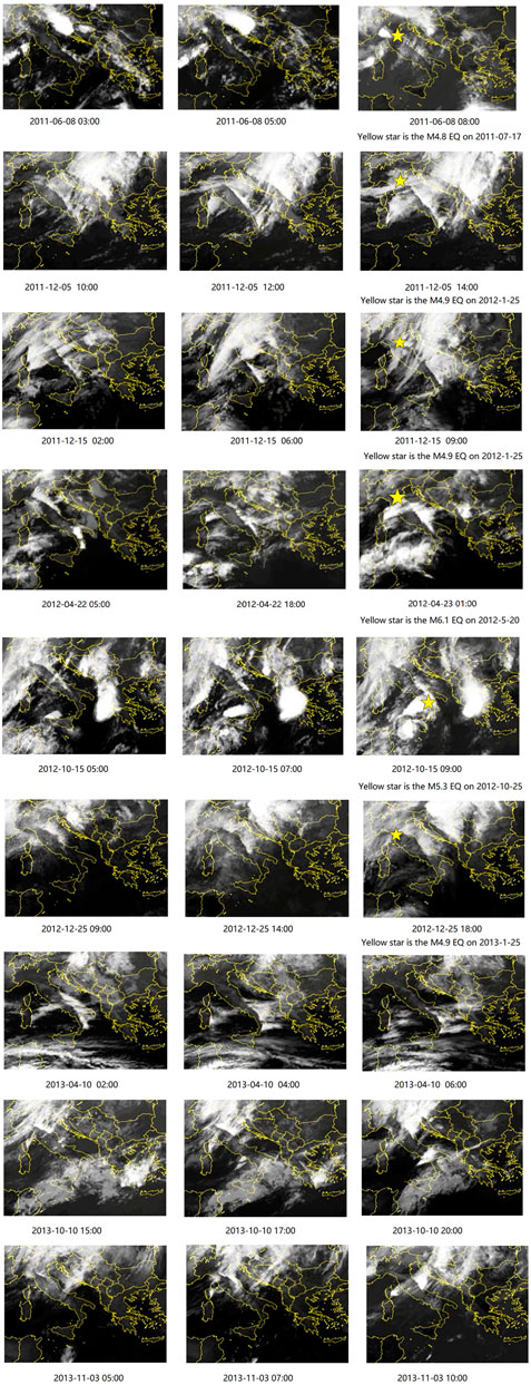
FIGURE 1. Typical satellite cloud anomalies appeared over Italy main fault systems. The yellow star means the earthquake following the cloud anomaly. Note some cloud anomalies has no earthquake that followed.

Data and Method

The cloud data is derived from Thomas et al. (2015) and the sat24 website (Table 1). All the stationary clouds which stayed bigger than 3 h are selected as candidate anomalies. Some typical clouds are listed in Figure 1 and others are listed in supplement files which derived from EUMETSAT. Earthquake data is derived from EMSC (Table 2). First we defined two parameters, EQ (earthquake) occurrence rate (EOR) and the anomaly appearance rate (AAR). AAR is defined by the number of EQs which occurred within the leading time interval ΔT after cloud anomaly appearance divided by the total number of EQs, whereas EOR is the number of cloud anomalies which preceded EQs within the same leading time interval ΔT divided by the total number of cloud anomalies. Note that AAR and EOR are equivalent to the alarm rate and success rate in earthquake prediction (Orihara et al., 2012).

TABLE 1

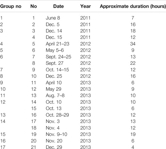
TABLE 1. Cloud anomalies in Italy and their duration in 2010–2013.

TABLE 2

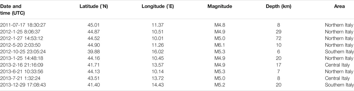
TABLE 2. Earthquakes in 2010–2013 with M ≥ 4.7 in the land area of Italy.

Second we calculated EOR and AAR for the earthquakes in Italy. Tronin (2000) and Tronin et al. (2002) studied AVHRR satellite thermal infrared data and found thermal anomalies 6–24 days before earthquakes with magnitude bigger than or equal to M4.7. All of the earthquakes bigger than or equal to M4.7 in Italy land area in 2010–2013 were selected from EMSC (http://www.emsc-csem.org). In this period, some events in the Corsica Sea and Ionian Sea were excluded because this study concerns only the land earthquakes. Finally we got the 10 earthquakes listed in Table 2, and their epicenters are reported in Figure 2.

FIGURE 2

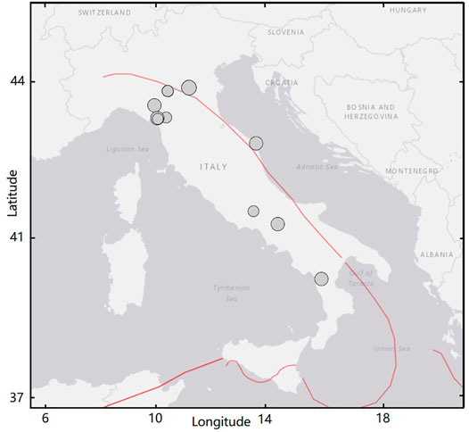
FIGURE 2. Map of the 10 earthquakes that happened in land of Italy from 2010 to 2013 with M ≥ 4.7. The red line is the main fault systems of Italy.

Statistical Analysis

The aftershocks for the M6.1 earthquake occurred on 20 May 2012, were clustered into one group with the main shock. Similarly we clustered cloud anomalies within three consecutive days into one group and finally got 17 groups of cloud anomalies. Figure 3 shows the time series of cloud anomalies and earthquakes.

FIGURE 3

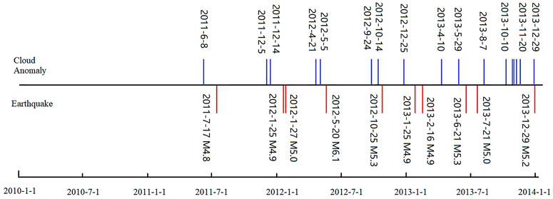
FIGURE 3. Time series of cloud anomalies and earthquake occurrences in Italy during 2010–2013.

To prove that AAR was not obtained by chance, we compared the actual values of AAR with that of temporally randomly generated EQs. In this study 10 EQs were randomly inserted into 1,461 days (namely 365 × 4 + 1), and 10,000 catalogues were generated by the Mersenne Twister algorithm (Matsumoto et al., 1998). Then AAR was calculated for the randomly generated catalogue for a different leading time interval, and the result is shown in Figure 4 (top). It was clear that the actual values of AAR were much higher than those expected by chance except ΔT≤30 days. For the case of 23≤ΔT≤45 days, it used the minimum time interval, namely 23 days, and got the maximum AAR 70%.

FIGURE 4

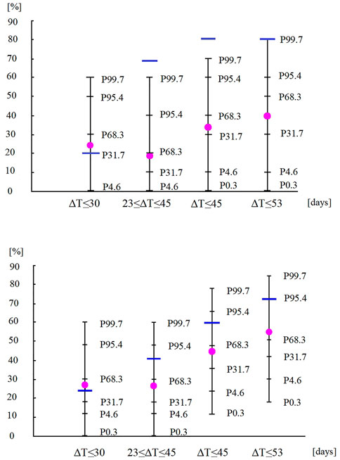
FIGURE 4. AAR (top) in the randomly generated catalogue and EOR (bottom) in the randomly generated cloud anomalies. Magenta points denote the mean value of the simulated data; short horizontal bars indicate percentiles of simulated data and blue bars indicate the actual value of real data. Clearly the actual values of AAR and EOR are higher than those expected by chance except ΔT≤30 days.

As for EOR, the EQ dates were fixed, 17 cloud anomalies were randomly inserted into 1,461 days, and finally 10,000 model sets were generated by the Mersenne Twister algorithm. The calculated EOR values for these sets for different ΔT are shown in Figure 4 (bottom). It was also clear that the actual values were much higher than those for random models except ΔT≤30 days. For the case of 23≤ΔT≤45 days, it used the minimum time interval, namely 23 days, and got EOR 41.2%. Thus it was statistically demonstrated that the relation between cloud anomaly and Italy land EQs was nearly impossible to be obtained by chance, and some correlation should exist.

We noticed that nearly all the earthquakes of Table 2 were preceded at least by one anomaly from 23 to 45 days before their occurrence, except three events happened on 2013-1-25, 2013-2-16, and 2013-7-21. The epicentre of the last one was located in the coast of the Adriatic Sea, so the presence of sea-layer could alter the possible mechanism of generation of the precursory anomaly to the atmosphere. The other events of January and February 2013 were characterized by a low magnitude, even if an anomaly has preceded other events of the same energy. The tectonic region of the event of 2013-1-25 is a bit different from the other events, and this could be also a possible reason for the lack of the anomaly in the leading time.

We checked the relationships for cloud anomalies related to leading time T (unit:days), which is the time in advance between the cloud anomaly and the EQ occurrence, and the cloud anomaly duration D (unit:hours) with the EQ magnitude M. The results showed that the relation between EQ magnitude and leading time T is not significant. This looks different from previous research results, so more investigations are needed in the future to check this point. While EQ magnitude is found to be strongly related with cloud anomaly duration, and the linear regression equation is D = 22.812M-101.52 with R² = 0.6992 (Figure 5). An interesting point is, the duration of the cloud anomaly on April 21–23, 2012, is the only one which is bigger than 2δ and 3δ compared with all the cloud duration in 2010–2013, and the earthquake that happened on 20 May 2012, is the biggest one in 2010–2013 (Guo, 2021). This means the cloud anomaly appeared on April 21–23, 2012, is related with the Emilia M6.1 earthquake with very high confidence (>99% level).

FIGURE 5

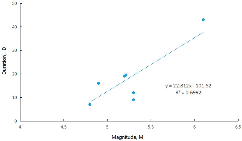
FIGURE 5. Linear regression of cloud anomaly duration and Magnitude.

Magnitude is usually estimated with ± 0.2 uncertainty, so we also checked the case of M4.5 and M4.9 from EMSC catalogue. If M4.5 threshold is used, there are two more earthquakes that appeared compared to the M4.7 threshold. They are M4.6 in north Italy on 14:41:30, 2012–10–3, and M4.6 in north Italy on 15:01:33, 2013-6-23. The second one is the aftershock of 2013-6-21 M5.3 earthquake, and as we point out in the text, it should be clustered into one group with the main shock, so it does not affect the result. The first earthquake is a new one, so the total number will be 11 earthquakes. Because there is a cloud anomaly on 2012-9-27, which is 6 days before the earthquake, AAR will be 0.727, EOR will be 0.471, both increased. If M4.9 threshold is used, the M4.8 earthquake on 2011-7-17 will be deleted, and then the total number will be nine earthquakes. AAR will be 0.66, and EOR will be 0.35, which is very close to the result of Perrone et al. (2018).

For the USGS catalogue, if M4.7 threshold is used, the total number will be 12 earthquakes. The two new earthquakes are M4.7 in north Italy on 2012-3-5 and M4.7 in central Italy on 2012-3-15, and both have no cloud anomaly. So AAR will be 7/12 = 0.583, and EOR will not change. If M4.9 threshold is used, the M4.8 earthquake (reported by USGS) on 2013-2-16, which has no cloud anomaly, will be deleted, and then the total earthquake number will be 9. AAR is 7/9 = 0.77, EOR will not change. If M4.5 threshold is used, the total number will be 16 earthquakes, then AAR is 11/16 = 0.68, and EOR is 11/17 = 0.64. The statistics for the EMSC catalogue and USGS catalogue show that AAR and EOR are both significant for the case of 23≤ΔT≤45 days. This proves that cloud method is convincing even for different catalogues.

Forecast Possibilities of the Method

Table 3 presents the error matrix for the investigated period. The total alerted time is 391 days compared with 1,461 total days, so the ratio is 26.7%. The time windows without cloud anomalies which are not followed by an earthquake is estimated as the number of not-alerted days (i.e., 1,070) divided by the width of the alerted window (23 days) and subtracting the three not-predicted earthquakes. Based on this table it is possible to define the overall accuracy of the method as the sum of the total correct case (earthquake preceded by cloud anomaly in the proper time + absence of cloud anomaly and earthquake) divided by the total case (Fawcett, 2006), and it is equal to 75% which indicates that the method is better than a prediction made by chance that would give 50% of accuracy.

TABLE 3

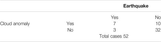
TABLE 3. Error matrix for the statistical evaluation of the cloud anomalies 23–45 days before the M ≥ 4.7 earthquakes in Italy during 2010–2013.

To compare the performance of cloud method and other methods, we selected two research reports made by Piscini et al. (2017) and Piscini et al. (2017). Perrone et al. (2018) analysed skin temperature (skt), total column water vapour, and total column of ozone changes before five earthquakes in central Italy between July and October from 1994 to 2016. Perrone et al. (2018) analysed ionospheric anomalies and 15 earthquakes with M ≥ 6.0 in the Greece area from 2003 to 2015. The EOR, AAR, the False alarm rate (F) and the overall accuracy (Acc) of these three methods are listed in Table 4. The false alarm rate is the number of anomalies without a following earthquake divided by the total alarm; the closer to 0, the better the value. In our case F = 10/(10 + 32) = 0.238.

TABLE 4

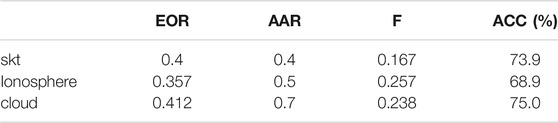
TABLE 4. Comparison of performance of three methods.

Table 4 shows that all the three methods provide similar EOR ranging from 0.357 to 0.412, and similar overall accuracy ranging from 68.9% to 75%. The false alarm rate of cloud method (0.238) is similar to that of ionosphere method (0.257), but a little higher than that of skt method (0.167). A clear difference is that the AAR of cloud method is bigger than that of the other two methods. It means that cloud method shows a better performance. If these three methods are combined together, as Piscini et al. (2017) did and combined three kinds of climate data, the final performance will increase greatly.

Japan scientists Orihara et al. (2012) used Greece VAN method (Varotsos et al., 1986) to monitor the telluric current signals observed in Kozu-Shima Island of Japan. They got 19 anomalies and 23 earthquakes in 1,139 days, and 11 quakes were preceded by a telluric current anomaly. The average earthquake frequency for this area was 1,139/23 = 49.52 days. They found that the best correlation existed for the case of ΔT≤30 days, so the time ratio is 30/49.52 = 0.606. Our method got 17 anomalies and 10 earthquakes in 1,461 days in Italy, and seven earthquakes were preceded by cloud anomalies for the case of 23≤ΔT≤45 days. The average earthquake frequency was 1,461/10 = 146.1 days. Our leading time interval was 23 days, and then the ratio was 23/146.1 = 0.157. It was much smaller than the alarm window of Japan scientists’ telluric current method (0.606). This means cloud method used a shorter leading time interval and gave a better performance than telluric current method.

Discussion

Thomas et al. (2015) studied the relation between clouds and earthquakes in Italy with Kuiper test method, and they considered that there was no significant relation between clouds and M ≥ 5.0 earthquakes. In their research they set an integer M5.0 as threshold without reasonable reason, and this subjective data selection strategy would lead to different conclusion; another problem was that Kuiper test will underestimate the result when many aftershocks appeared. Here we used EOR and AAR model and proved that clouds anomaly had significant relation with M ≥ 4.7 earthquakes in the Italy land area. These two models are widely accepted by the seismic community, and the threshold is selected based on previous studies which are widely used in thermal anomaly research, so the result is convincing.

Preseismic clouds could be mixed with orographic clouds. Someone may consider that when water vapor travels from sea to Italy land area, it climbs up the mountains and the clouds form when the temperature decreases. Satellite data show that the altitude of preseismic clouds is about 10,000 m, while the Italy Appenin mountains are just about 2000 m high (for example, the highest Appenin Mount is 2,492 m). If the water vapor climbs up the mountains from sea surface to 2000 m, then it cannot rush to an altitude of about 10,000 m. So a new physical mechanism needs to be involved, and the seismic source could be one. Scientists have put forward some possible mechanisms, for example, Japanese scientists Teramoro and Ikeya (2000) used 4 kv/m electric field in a Wilson’s cloud chamber and produced some linear clouds. American scientists (Freund et al., 2007; Freund, 2010) found that electronic charge carriers would be activated when rocks were stressed, and this would create an electric field which could be strong enough to ionize air molecules. The airborne ions could act as condensation nuclei for water droplets and then lead to fogs and clouds. British scientists (Harrison et al., 2014) used Atmospheric Lithosphere-Ionosphere Charge Exchange (ALICE) model to show that the global circuit conduction current can connect surface air ionisation changes to the properties of the cloud above in semi-fair weather directly. Pulinets et al. (2015) proposed a LAI (Lithosphere-Atmosphere-Ionosphere) coupling model and tried to explain this phenomenon by a complex chain of sub-processes starting from the release of ionized particles from the stressed fault. They considered that radon gas would emit from activated faults, and the vertical electric field above the faults supports the linear structure of cluster ion flows which leaded to the formation of anomalous linear clouds. All these studies from different countries provide some possible physical mechanism which connected active fault, electric field, and cloud anomaly.

Conclusion

In this paper we used 4 year satellite data and a statistics model and provide a strong evidence that clouds had significant relation with earthquakes in the Italy land area in 2010–2013. Our result showed that when the leading time interval was set to 23≤ΔT≤45 days, seven of the total 10 earthquakes were preceded by cloud anomalies. The methods alerted a relative short time window (26.7%) and gave an overall accuracy equal to 75%. The disadvantage of this method was that the cloud anomaly was very long and it cannot estimate the epicenter location accurately. So here we suggested combing some other geophysical data and method such as VAN method (Varotsos et al., 1986), latent heat flux method (Dey and Singh, 2003), satellite thermal method (Pulinets et al., 2014), magnetic method (De Santis et al., 2017), etc. to increase the prediction accuracy. For example, Qin et al. (2012) found thermal anomaly appeared in north Italy on 12 May 2012, and if combined with the cloud anomaly which appeared on April 23, 2012, then the prediction accuracy could be promoted greatly. In future development, cloud method could be applied to other areas to test where and if it can be applied.

Data Availability Statement

The original contributions presented in the study are included in the article/Supplementary Material, further inquiries can be directed to the corresponding author.

Author Contributions

The author confirms being the sole contributor of this work and has approved it for publication.

Funding

This work was supported by Natural Science Foundation of Henan (182300410141).

Conflict of Interest

The author declares that the research was conducted in the absence of any commercial or financial relationships that could be construed as a potential conflict of interest.

Publisher’s Note

All claims expressed in this article are solely those of the authors and do not necessarily represent those of their affiliated organizations, or those of the publisher, the editors and the reviewers. Any product that may be evaluated in this article, or claim that may be made by its manufacturer, is not guaranteed or endorsed by the publisher.

Acknowledgments

Four reviewers gave valuable comments and suggestions on this paper. Their kind help is greatly appreciated.

Supplementary Material

The Supplementary Material for this article can be found online at: https://www.frontiersin.org/articles/10.3389/feart.2022.812540/full#supplementary-material

References

De Santis, A., Balasis, G., Pavón-Carrasco, F. J., Cianchini, G., and Mandea, M. (2017). Potential Earthquake Precursory Pattern from Space: the 2015 Nepal Event as Seen by Magnetic Swarm Satellites. Earth Planet. Sci. Lett. 461, 119–126. doi:10.1016/j.epsl.2016.12.037

CrossRef Full Text | Google Scholar

Dey, S., and Singh, R. P. (2003). Surface Latent Heat Flux as an Earthquake Precursor. Nat. Hazards Earth Ssyst. Sci. 3, 749–755. doi:10.5194/nhess-3-749-2003

CrossRef Full Text | Google Scholar

Fawcett, T. (2006). An Introduction to ROC Analysis. Pattern Recognition Lett. 27, 861–874. doi:10.1016/j.patrec.2005.10.010

CrossRef Full Text | Google Scholar

Freund, F. (2010). Toward a Unified Solid State Theory for Pre-earthquake Signals. Acta Geophys. 58 (5), 719–766. doi:10.2478/s11600-009-0066-x

CrossRef Full Text | Google Scholar

Freund, F. T., Takeuchi, A., Lau, B. W. S., Al-Manaseer, A., Fu, C. C., Bryant, N. A., et al. (2007). Stimulated Infrared Emission from Rocks: Assessing a Stress Indicator. eEarth 2, 7–16. doi:10.5194/ee-2-7-2007

CrossRef Full Text | Google Scholar

Guo, G. (2021). A Retrospective Analysis about the Italy Emilia M6.0 Earthquake Prediction. Ojer 10, 68–74. doi:10.4236/ojer.2021.102005

CrossRef Full Text | Google Scholar

Guo, G. M., and Yang, J. (2013). Three Attempts of Earthquake Prediction with Satellite Cloud Images. Nat. Hazards Earth Syst. Sci. 13, 91–95. doi:10.5194/nhess-13-91-2013

CrossRef Full Text | Google Scholar

Guo, G., and Wang, B. (2008). Cloud Anomaly before Iran Earthquake. Int. J. Remote Sensing 29, 1921–1928. doi:10.1080/01431160701373762

CrossRef Full Text | Google Scholar

Harrison, R. G., Aplin, K. L., and Rycroft, M. J. (2014). Brief Communication: Earthquake-Cloud Coupling through the Global Atmospheric Electric Circuit. Nat. Hazards Earth Syst. Sci. 14, 773–777. doi:10.5194/nhess-14-773-2014

CrossRef Full Text | Google Scholar

Mansouri Daneshvar, M. R., Tavousi, T., and Khosravi, M. (2014). Synoptic Detection of the Short-Term Atmospheric Precursors Prior to a Major Earthquake in the Middle East, North Saravan M 7.8 Earthquake, SE Iran. Air Qual. Atmos. Health. 7, 29–39. doi:10.1007/s11869-013-0214-y

CrossRef Full Text | Google Scholar

Matsumoto, M., Nishimura, T., and Mersenne, T. A. (1998). Mersenne Twister. ACM Trans. Model. Comput. Simul. 8 (1), 3–30. doi:10.1145/272991.272995

CrossRef Full Text | Google Scholar

Morozova, L. I. (1997). Dynamics of Cloudy Anomalies above Fracture Regions during Natural and Anthropogenically Caused Seismic Activities. Fizika Zemli 9, 94–96.

Google Scholar

Orihara, Y., Kamogawa, M., Nagao, T., and Uyeda, S. (2012). Preseismic Anomalous Telluric Current Signals Observed in Kozu-Shima Island, Japan. Proc. Natl. Acad. Sci. U S A. 109, 19125–19128. doi:10.1073/pnas.1215669109

PubMed Abstract | CrossRef Full Text | Google Scholar

Perrone, L., De Santis, A., Abbattista, C., Alfonsi, L., Amoruso, L., Carbone, M., et al. (2018). Ionospheric Anomalies Detected by Ionosonde and Possibly Related to Crustal Earthquakes in Greece. Ann. Geophys. 36, 361–371. doi:10.5194/angeo-36-361-2018

CrossRef Full Text | Google Scholar

Piscini, A., De Santis, A., Marchetti, D., and Cianchini, G. (2017). A Multi-Parametric Climatological Approach to Study the 2016 Amatrice-Norcia (Central Italy) Earthquake Preparatory Phase. Pure Appl. Geophys. 174 (10), 3673–3688. doi:10.1007/s00024-017-1597-8

CrossRef Full Text | Google Scholar

Pulinets, S. A., Morozova, L. I., and Yudin, I. A. (2014). Synchronization of Atmospheric Indicators at the Last Stage of Earthquake Preparation Cycle. Res. Geophys. 4 (1), 45–50.doi:10.4081/rg.2014.4898

CrossRef Full Text | Google Scholar

Pulinets, S. A., Ouzounov, D. P., Karelin, A. V., and Davidenko, D. V. (2015). Physical Bases of the Generation of Short-Term Earthquake Precursors: A Complex Model of Ionization-Induced Geophysical Processes in the Lithosphere–Atmosphere– Ionosphere–Magnetosphere System. Geomagnetism and Aeronomy 55 (4), 540–558. doi:10.1134/s0016793215040131

CrossRef Full Text | Google Scholar

Qin, K., Wu, L. X., De Santis, A., and Cianchini, G. (2012). Preliminary Analysis of Surface Temperature Anomalies that Preceded the Two Major Emilia 2012 Earthquakes (Italy). Ann. Geophys. 55, 823–828. doi:10.4401/ag-6123

CrossRef Full Text | Google Scholar

Shou, Z. H. (1999). Earthquake Clouds, a Reliable Precursor. Sci. Utopya 64, 53–57.

Google Scholar

Teramoro, K., and Ikeya, M. (2000). Experiment Study of Cloud Formation by Intense Electric fields. J. Appl. Phys. 5, 2876–2881. doi:10.1143/JJAP.39.2876

CrossRef Full Text | Google Scholar

Thomas, J. N., Masci, F., and Love, J. J. (2015). On a Report that the 2012 M 6.0 Earthquake in Italy Was Predicted after Seeing an Unusual Cloud Formation. Nat. Hazards Earth Syst. Sci. 15, 1061–1068. doi:10.5194/nhess-15-1061-2015

CrossRef Full Text | Google Scholar

Tronin, A. A., Hayakawa, M., and Molchanov, O. A. (2002). Thermal IR Satellite Data Application for Earthquake Research in Japan and China. J. Geodynamics 33, 519–534. doi:10.1016/s0264-3707(02)00013-3

CrossRef Full Text | Google Scholar

Tronin, A. A. (2000). Thermal IR Satellite Sensor Data Application for Earthquake Research in China. Int. J. Remote Sensing 21, 3169–3177. doi:10.1080/01431160050145054

CrossRef Full Text | Google Scholar

Varotsos, P., Alexopoulos, K., Nomicos, K., and Lazaridou, M. (1986). Earthquake Prediction and Electric Signals. Nature 322, 120. doi:10.1038/322120a0

CrossRef Full Text | Google Scholar

Wu, L. X., Li, J. P., and Liu, S. J. (2009). “Space Observed Two Abnormal Linear Clouds before Wenchuan Earthquake,” in Proceedings of the 3rd IASME/WSEAS International Conference of Geology and Seismology. February 24-26, 2009. Cambridge, United Kingdom, 138–143.

Google Scholar