Microbial Methane Generation and Implications for Stability of Shallow Sediments on the Upper Slope, U.S. Atlantic Margin

1 Introduction

Methane hydrates are solid, crystalline structures composed of methane and water. Hydrates are stable in an environment with low temperature, high pressure, and where sufficient methane is present (Kvenvolden and Claypool, 1988). Hydrates are stable beneath the seafloor when the bottom water temperature approaches 0°C and the water depth is greater than 300 m (Kvenvolden and Lorenson, 2001). The depth range at which methane hydrates are stable is known as the gas hydrate stability zone (GHSZ). The GHSZ continues below the seafloor to the base of the hydrate stability zone (BHZ) where the hydrate phase envelope intersects the geotherm. The depth of the BHZ can be found up to 2000 m below the seafloor but is typically found at much shallower depths (Kvenvolden, 1993).

An increase in local temperature or decrease in local pressure can cause destabilization and the subsequent dissociation of hydrates (Phrampus and Hornbach, 2012; Ruppel and Kessler, 2017). Methane gas released due to hydrate dissociation can migrate up to the seafloor and into the water column. In the water column, it can oxidize into CO₂ causing ocean acidification, or it may continue through the water column and into the atmosphere as a greenhouse gas (Biastoch et al., 2011). Increasing temperatures and the subsequent dissociation of hydrate is especially a concern at the BHZ where the in-situ pressure and temperature conditions intersect the hydrate phase envelope and even minor changes in temperature can cause hydrate dissociation. There is evidence that within the last 100 years, increases in global ocean temperatures have led to hydrate instability and the shifting of the hydrate stability zone along the Beaufort shelf and off the Svalbard coast (Ferré et al., 2012; Sarkar et al., 2012; Phrampus et al., 2014). In shallower water (around 500 m) where the BHZ is at or near the seafloor, also known as the feather edge, the increase in seafloor temperature is problematic (Ruppel, 2011). As water depth increases, this becomes less of an issue as the GHSZ thickens. In shallow marine sediments within 132 m of the seafloor, the presence of gas can lead to tensile fracturing in the sediments, and gas in these shallower sediments can occupy a much larger volume than hydrate under the same conditions (Daigle et al., 2020).

We are interested in the geomechanical properties of the seafloor sediment when methane gas is formed due to hydrate dissociation from increasing temperatures. We focus specifically on the feather edge where the hydrate stability zone is the thinnest. To begin, we model TOC along the U.S. Atlantic margin. At a few locations where estimated seafloor TOC is high, we use a 1D sediment burial and methanogenesis model to simulate hydrate and gas formation over a 120,000 years glacial cycle. At locations along the feather edge, we assume a 1°C increase in temperature at the BHZ and model the geomechanical response of the system as hydrate dissociates to methane gas and water. We are interested in determining if the conditions for sediment failure due to an increase in temperature can exist under the right circumstances. Thus, at each location we calculate a Hoek-Brown failure envelope to determine if failure occurs due to dissociation.

2 Background

Ocean Drilling Program (ODP) boreholes give an insight into locations where methane gas and methane hydrate occur along the U.S. Atlantic margin. Along the upper continental slope, offshore of New Jersey, ODP boreholes report subsurface microbial methane, indicating methanogenesis in the area (Shipboard Scientific Party, 1994a; Shipboard Scientific Party, 1994b; Shipboard Scientific Party, 1994c; Shipboard Scientific Party, 1994d; Shipboard Scientific Party, 1994e; Shipboard Scientific Party, 1998a). South of this region, offshore of North Carolina and South Carolina, seismic profiles from the ODP show a strong bottom-simulating reflector (BSR) at some locations, inferring the presence of hydrate in the area (Shipboard Scientific Party, 1996b; Shipboard Scientific Party, 1996c; Holbrook et al., 1996; Dickens et al., 1997).

In sediment near the seafloor, gas-driven tensile failure can occur due to a combination of low stresses and weak sediments. Fine grained sediments with a higher clay fraction are more prone to failure as gas within these sediments has a higher capillary pressure. Therefore, less gas is required to be present to cause failure (Daigle et al., 2020). One mechanism for gas generation is the dissociation of methane hydrates although gas generated directly from microbial methanogenesis can also lead to tensile failure.

The release of methane gas from the seafloor can be seen in water column acoustic anomalies which correspond to gas plumes (Judd, 2003; Skarke et al., 2014). In global surveys summarizing free gas distribution in marine sediments, Fleischer et al. (2001) and Judd (2003) both note occurrences of free gas along the U.S. Atlantic margin. The release of gas is evident in the development of pockmarks on the seafloor which form due to the accumulation of gas beneath a seal, and the subsequent release of gas when the seal fails (Cathles et al., 2010; Brothers et al., 2014; Sultan et al., 2014). Along the U.S. Atlantic margin, pockmarks just shallow of the feather edge were reported by Brothers et al. (2014). In addition, asymmetric depressions corresponding to elongated gas blowouts were reported by Hill et al. (2004) along the U.S. Atlantic margin.

Investigations by Skarke et al. (2014) found instances of methane gas leakage from the seafloor along the U.S. Atlantic margin at a higher concentration than previously thought. Skarke et al. (2014) identified 570 gas plumes on the northern U.S. Atlantic margin, with 440 of these seeps (77%) lying between the shelf break (∼180 m below sea level) and 600 m below sea level. The location of these plumes would lie just updip of the feather edge of the GHSZ. The seeps in this area were further explored by Prouty et al. (2016) who suggest that seepage may have begun as early as 15 kya in the Baltimore Canyon seep field, and between one to three kya at the deeper Norfolk seep field (Figure 1). Gas seeps in this region have δ¹³C values between –73.5‰ and –109‰ and methane:ethane ratios between 385 and 926 indicating that the gas is microbial in origin (Pohlman et al., 2017).

FIGURE 1

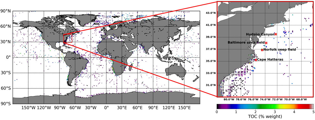
FIGURE 1. Known measurements of total organic carbon (TOC) globally and within the area 29°N–45°N and 82°W–66°W. In the zoomed in region, the locations of Hudson Canyon, Baltimore seep field, Norfolk seep field, and Cape Hatteras are also indicated.

3 Materials and Methods

The Global Predictive Seabed Model (GPSM) was used to model and create maps of total organic carbon (TOC) and porosity at the seafloor. In areas with high predicted values of TOC, we used Dakota and PFLOTRAN to model the generation of methane gas and hydrate due to methanogenesis and the burial of the seafloor sediment. In locations where the BHZ was close to the seafloor, we modeled the geomechanical response of sediment to gas generated by hydrate dissociation to better understand whether shear failure or tensile failure would occur. We specifically focused on hydrate dissociation caused by an increase in temperature at the BHZ. The hydrate formed through the PFLOTRAN model and subsequently dissociated in the geomechanical model was assumed to be structure I methane hydrate.

3.1 The Global Predictive Seabed Model

GPSM is a geospatial machine learning model developed by the Naval Research Laboratory and can be used to predict TOC, porosity, sediment composition, and other properties of seafloor sediments in areas where no measurements have been sampled or recorded (Martin et al., 2015). GPSM offers a variety of machine learning methods to create geospatial models including k-nearest neighbor regression, support vector regression, and random forest regression. In these geospatial machine learning models, predictions do not assume spatial autocorrelation. Instead, the characteristics or parameters of locations are compared rather than the geographic proximity of two points.

3.1.1 Modeling Seafloor Total Organic Carbon

To model seafloor TOC, we followed the methodology of Lee et al. (2019) and used a k-nearest neighbor (kNN) approach. For our model, a value of k = 5 was chosen. When predicting TOC values on the seafloor at unknown locations, GPSM compares various observed attributes of the unknown location with the same observed attributes at locations with known TOC values. These observed attributes are known as predictors and are found in global grids known as predictor grids. In our model 1749 predictor grids were used including data from multiple global surveys such as seamount censuses, global river fluxes of carbon and sediments to the ocean, and decadal trends in oxygen concentration in subsurface waters, among others (Phrampus et al., 2020). Therefore, our model differs slightly from that of Lee et al. (2019) as we are using both new and additional predictor grids.

In our model, 5,595 individual locations with known TOC values were sampled (Seiter et al., 2004). These are from the upper 5 cm of sediment and so are roughly Pleistocene in age. Of these, we excluded values of TOC over 5% to mitigate outliers in the predictions. We then averaged values for each 5 × 5 arc-minute grid cell to obtain a uniformly spaced grid. Of the 5,595 locations with known TOC, 126 points had measurements greater than 5% TOC (2.2% of the data) and were excluded. After creating a uniformly spaced grid, 4,879 useable observations remained (Figure 1).

We used tenfold validation to validate our model. In tenfold validation, the data is first randomly split into 10 equal sized groups. One group is excluded as a test set and the remaining 90% of the data is used to form a training set. A model (in this case kNN) is created using the training set of data and then tested on the remaining 10% of the data where the predicted value from the model can be compared to the actual value of the test set. This process is done 10 times. Plotting the observed versus predicted data values gives us the validation graph in Figure 2. The validation of this data shows an R² value of 0.6151, lying below the ideal 1:1 fit at high observed TOC values. Other k values between 3 and 20 were tested to optimize for the highest R² value. We chose k = 5 for our model as it was among the top performing models and is consistent the work done by Lee et al. (2019).

FIGURE 2

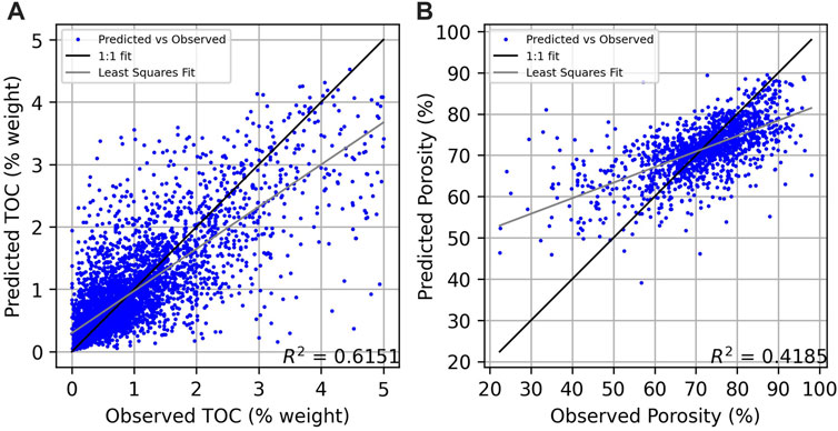
FIGURE 2. Validation plot of (A) observed TOC values versus predicted TOC values for the k-nearest neighbor model (k = 5) and (B) observed porosity values versus predicted porosity values for the random forest model using 100 trees and a minimum samples per leaf of 3. The 1:1 fit line shows where observed values match the predicted values. The least squares regression fit of the model is depicted by the gray line.

After forming a model using tenfold cross validation, we checked the predictor grids for collinearity. Grids with a correlation coefficient over 0.99 were removed, leaving 1,622 of the 1,749 predictor grids. In addition, an error grid was used to remove predictor grids with high error. Since this grid is made of random, uniform noise, it should have no influence on the data being modelled. The predictors grids can be ordered by individual error and any predictor grids with a higher error than the noise grid is ignored and not used in the model. This left us with 1,618 predictor grids which were used for the prediction. TOC predictions were made on the 5 × 5 arc-minute grid within the area 29°N–45°N and 82°W–66°W (Figure 1).

3.1.2 Modeling Seafloor Porosity

We also used GPSM to model seafloor porosity in our region of interest. The same 1,749 predictor grids used to predict seafloor TOC were used in our seafloor porosity model. In this model, 2027 individual locations with known seafloor porosity values were sampled (Martin et al., 2015). Of these, values of porosity over 90% and below 20% were excluded and the remaining values were averaged for each 5 × 5 arc-minute grid leaving us with 1,440 useable observations. Both a kNN approach and a random forest regression (RFR) approach were modeled. The RFR methodology followed a similar workflow to the work done by Graw et al. (2021) and is similar to the work done to predict seafloor TOC. As we previously did, we used a tenfold cross validation method to determine model variation. A similar validation plot to TOC was calculated for both the kNN and RFR methods using tenfold validation for seafloor porosity. A maximum R² value for the RFR method was calculate using 100 trees and a minimum samples per leaf of 3 (Figure 2). Although this R² value (0.4185) was less than the R² value for the kNN test (0.4562), we chose to use the RFR model due to lower standard deviations of the porosity predictions at our points of interest.

3.2 Dakota and PFLOTRAN

Dakota and PFLOTRAN were used to model the burial of seafloor sediments and the resulting generation of methane hydrate and methane gas in an approach similar to Eymold et al. (2021). Both Dakota and PFLOTRAN are open-source software developed by Sandia National Laboratories. Dakota was developed to provide optimization tools for simulations and we used it to sample PFLOTRAN input parameters, creating a distribution of model results (Adams et al., 2021).

PFLOTRAN is a parallel subsurface flow code which solves a system of nonlinear partial differential equations describing flow and transport in porous medium (Hammond et al., 2014). Following the work of Eymold et al. (2021) and Nole et al. (2017), we used PFLOTRAN to simulate hydrate and gas formation from microbial gas during sediment burial. Eymold et al. (2021) and Nole et al. (2017) use a primary variable switch method to solve for mass and energy conservation with phase change (hydrate versus gas phase). The governing equations are set up as a finite volume difference discretization, and variables are then solved for in a fully implicit manner using a nonlinear Newton-Raphson iteration. The methane generation rate was calculated following Malinverno (2010):

$q\left(z\right)=k_{\alpha }\lambda \alpha \exp \left[-\frac{\lambda }{\omega }\left(z-z_{\text{SMT}}\right)\right](1)$

where q(z) is methane generation rate with depth in kg/m³/s, k_α = 2,241 kg/m³ is the conversion factor of TOC to methane, λ is the methanogenesis rate (s⁻¹), ω is the sedimentation rate (m/s), and z is the sediment depth (m). The depth of the sulfate-methane transition (z_SMT) was set at 15 m below seafloor (mbsf) based on work done by Malinverno (2010) and Egger et al. (2018). The metabolizable organic carbon remaining at the SMT (α) was set at 75% (Bhatnagar et al., 2007).

Initial conditions and boundary conditions for the simulation were also set up following the methodology of Eymold et al. (2021) and Nole et al. (2017). The initial conditions were set using Dirichlet temperature values, Dirichlet mole fraction values, and hydrostatic pressure at the seafloor. Temperature was set throughout the sediment column at a fixed temperature gradient from the seafloor. In addition, the mole fraction for methane in the aqueous phase was set to 0.001 along the entire profile. At the U.S Atlantic margin, there is documentation of gas in sediments as old as the Oligocene as well as deeper Mesozoic accumulations of thermogenic gas (Shipboard Scientific Party, 1994a; Shipboard Scientific Party, 1994b; Shipboard Scientific Party, 1994c; Shipboard Scientific Party, 1994d; Shipboard Scientific Party, 1994e; Party, 1998a; Shipboard Scientific Party, 1998a; Party, 1998b). However, since we were most interested in gas and hydrate close to the seafloor and the role of seafloor TOC in generating it, we chose to ignore the hydrate and gas that may already exist in the areas we model. At the bottom of the depth profile, Neumann boundary conditions were set such that the liquid and gas flux at the base of the profile were both 0, and heat flux at the boundary was equal to the heat flux sampled by Dakota. Since we were interested in the hydrate saturation near the feather edge, a maximum depth of 1,000 mbsf was used for our model. This ensured that the bottom boundary conditions (constant flux) did not directly influence hydrate and gas predictions at the feather edge.

3.3 Dakota and PFLOTRAN Inputs

We used PFLOTRAN to simulate methanogenesis and hydrate formation in a 1D model over time. A period of 120,000 years was chosen, representing the length of a glacial-interglacial cycle. Although this length of time was chosen to represent the glacial-interglacial cycle length, our goal was not to simulate the actual conditions over the last 120,000 years since many of the exact parameters and conditions are unknown to us. Even at the locations we are modeling, there are few constraints on the distribution and amount of gas and hydrate in the system. Therefore, we chose to model a variety of outcomes using Dakota to sample different initial seafloor conditions (TOC, porosity, sedimentation rate, and heat flux) while leaving other conditions such as seafloor temperature and pressure constant over time. This allowed us to get a general sense of how much gas and hydrate could form over a set amount of time which we then used as a basis to predict what might happen if the ocean warms. To set up this probabilistic model, Dakota was used to provide a distribution of results by sampling the PFLOTRAN input parameters TOC, sedimentation rate, heat flux, and porosity (Table 1). Specifically, Dakota used Latin hypercube sampling to provide a distribution of input variables that were modeled with PFLOTRAN. Table 1 summarizes the input variables used in the PFLOTRAN/Dakota model, with many values chosen following the work of Eymold et al. (2021).

TABLE 1

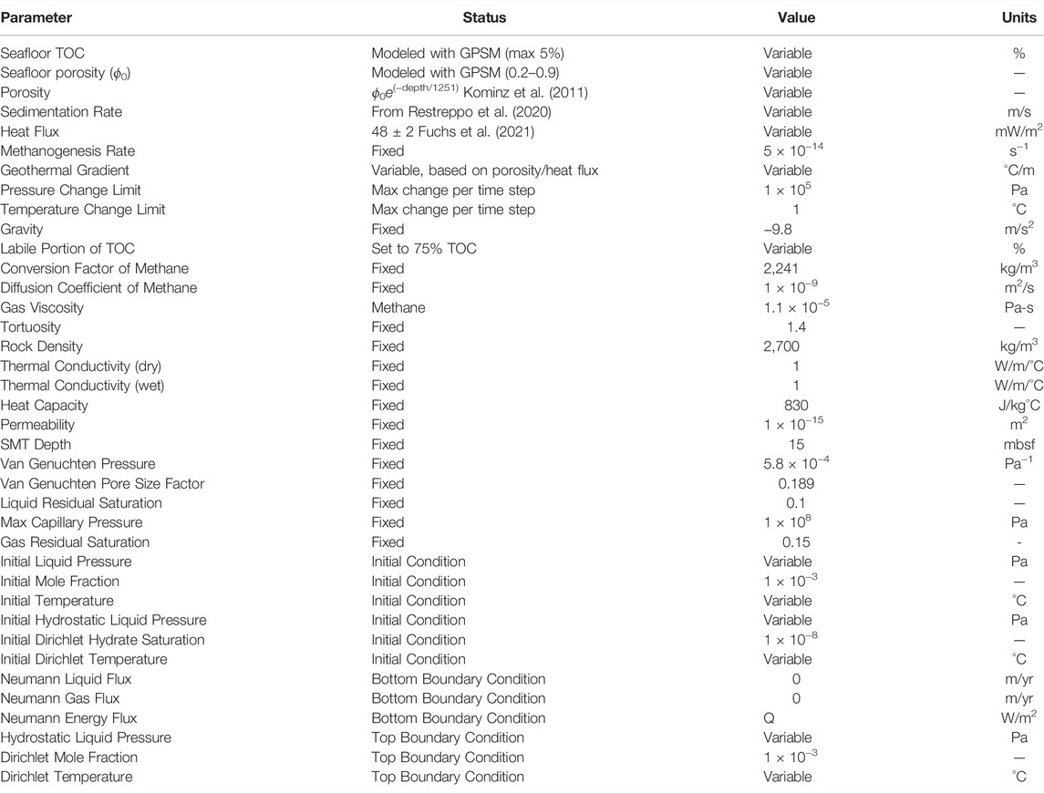
TABLE 1. Input parameters for Dakota and PFLOTRAN.

Dakota sampled TOC, sedimentation rate, heat flux, and seafloor porosity using a normal distribution. As previously discussed, TOC predictions and standard deviations were modeled using GPSM predictor grids from Phrampus et al. (2020) and observed data points from Seiter et al. (2004) (Figure 1). To avoid values of zero, a lower bound of TOC was set to 0.01%. An upper bound of TOC was set at 5%, like the GPSM model, to avoid unrealistically high values. Similarly, seafloor porosity was modeled using GPSM predictor grids from Phrampus et al. (2020) and observed data points from Martin et al. (2015). The lower and upper bounds on seafloor porosity were set to 20% and 90% respectively. At depth, porosity was calculated using the trend for marine silty clays presented by Kominz et al. (2011):

$\varphi \left(z\right)={\varphi }_0{e}^{-\frac{z}{1251}}(2)$

where ϕ is porosity. Here we assumed the regression of porosity followed the trend presented by Kominz et al. (2011), changing ϕ₀ to the value predicted at a given location in our region of interest. Sedimentation rates and standard deviations were determined from Restreppo et al. (2020) who modeled global oceanic sediment accumulation rates using GPSM at a 5 × 5 arc-minute resolution. Bounds on sedimentation rates were set to a minimum of 1 × 10⁻¹⁴ m/s (3.16 × 10⁻⁵ cm/yr) and to a maximum of 1 m/s. For the studied area, heat flux was sampled from Fuchs et al. (2021), and was set to 48 ± 2 mW/m². A methanogenesis rate of λ = 5 × 10⁻¹⁴ s⁻¹ was chosen based on estimates of λ = 1 × 10⁻¹⁴ s⁻¹ from Bhatnagar et al. (2007) and λ = 1 × 10⁻¹³ s⁻¹ from Malinverno (2010). This value for methanogenesis rate also lies between the constraints of 1 × 10⁻¹⁵ ≤ λ ≤ 1 × 10⁻¹³ s⁻¹ used by Eymold et al. (2021).

We focused our investigation on the area bounded by 36.6°N–38°N and 74.5°W–73.1°W. This area shows some of the higher TOC estimates in the modeled region. Table 2 summarizes the locations where PFLOTRAN and Dakota were used to model hydrate and gas generation. We picked four points along the strike of the continental shelf, located near the feather edge, and five locations along the shelf dip.

TABLE 2

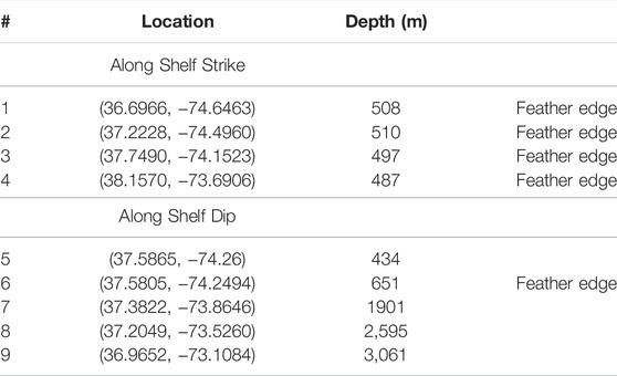
TABLE 2. Locations picked for PFLOTRAN/Dakota simulation.

At each location, the depth of the seafloor was determined with the Global Multi-Resolution Topography (GMRT) Synthesis (Ryan et al., 2009). The GMRT Synthesis provides high resolution bathymetry data for almost 10% of the global ocean. Individual locations can be queried through the GMRT PointServer Web Service to retrieve accurate water depths at specific latitude and longitude locations.

Seafloor temperatures were calculated at a given depth through a polynomial regression. Data from Boyer et al. (2018) provided 47 temperature profiles from conductivity-temperature-depth (CTD) casts within the 36.6°N–38°N and 74.5°W–73.1°W study area. Since the area of focus was the GHSZ feather edge, near the continental slope, a visual inspection of profile location was used to choose temperature profiles near the continental slope. This left 10 temperature profiles, and a 6^th order polynomial regression was used to create a model of water temperature for depths shallower than 1,000 m:

$\begin{array}{ll}\hfill T\left(z\right)& =5.450\text{x}10^{-16}{z}^6-1.641\text{x}10^{-12}{z}^5+1.763\text{x}10^{-9}{z}^4-7.746\text{x}10^{-7}{z}^3\hfill \\ \hfill & +1.075\text{x}10^{-4}{z}^2-8.606\text{x}10^{-3}z+12.504.\hfill \end{array}(3)$

As done with the initial conditions and boundary conditions, the other parameters in the PFLOTRAN model were chosen following the work of Eymold et al. (2021). Many of the values chosen are comparable to values measured at ODP wells in the region. For example, the thermal conductivity parameters for wet and dry sediment of 1 W/m/°C lie between the values found at ODP well site 1,073, ranging between 0.89 and 1.5 W/m/°C (Shipboard Scientific Party, 1998a). ODP wells (sites 902, 903, and 1,073) in this region have permeability measurements in the range of 10^–17 − 10^–16 m² (Blum et al., 1996; Dugan et al., 2003). However, we chose to use the permeability value of 10^–15 m² as done by Eymold et al. (2021) which can account for siltier beds that may occur in the region.

3.4 Geomechanics Model

Following the PFLOTRAN/Dakota simulation of sediment burial and methanogenesis two geomechanical models were used to simulate hydrate dissociation at the BHZ due to an increase in temperature. Our goal was to determine if the conditions needed for sediment failure can exist under the right circumstances, particularly for expected amounts of gas generated microbially, rather than determining the exact conditions needed for sediment failure.

As hydrate dissociates, gas pressure of the system increases causing a reduction in effective stress of the sediment. This can lead to elastic volumetric deformation of the sediment. Although some volumetric expansion will occur due to the increase in gas pressure, shallow marine sediments can still fracture and this fracturing behavior is well described by linear elastic fracture mechanics (Boudreau, 2012; Johnson et al., 2012). Since we are focused near the seafloor, at the feather edge, effective stresses will be small and we are unlikely to build up enough gas pressure to lead to large strains. Therefore, we chose to ignore the volumetric expansion of the sediment. Mechanics for plastic volumetric deformation due to hydrate dissociation have been discussed by Lee et al. (2010) and Waite et al. (2009). In sediments with hydrate saturations of 50–100% Lee et al. (2010) found a decrease in sediment porosity due to hydrate dissociation. However, Waite et al. (2009) discuss that S_h = 25% seems to be a threshold above which pore-filling hydrate becomes load-bearing hydrate. At low saturations, the pore-filling hydrate does not change the shear stiffness of the sediment (Waite et al., 2009). Therefore, in our model we will ignore plastic deformation and possible dilation during dissociation.

We focused specifically on the five hydrate bearing locations at the feather edge and modeled the drained and undrained responses that these sediments exhibit during loading. In the drained loading environment, water is allowed to flow out of the sediment during hydrate dissociation and the pore water pressure remains constant. Since the amount of gas formed during dissociation is small, we do not exceed the mobility threshold of gas (Daigle et al., 2020). Therefore, the gas formed will not dissipate through porous flow and will stay in the pore space. In an undrained loading environment, neither water nor gas are allowed to flow and the pore water pressure increases. In both the drained and undrained loading models, the initial pore space of the system was assumed to contain only hydrate and water. The hydrate dissociation reaction was assumed to go to completion (Eq. 4), leading to a final pore space containing only methane gas and water. In addition, no response to dissociation was modeled until the hydrate had fully dissociated to methane gas and water. In this way the final state of the system we model only includes gas and water in the pore space.

${\text{CH}}_4\cdot 5.75{\text{H}}_2\text{O}\to {\text{CH}}_4+5.75{\text{H}}_2\text{O}(4)$

In modeling the dissociation reaction only at start and at completion, we ignore changes in pressure within the system that can cause hydrate to reform as local pressure and temperature conditions change during deformation. In addition, we ignore the rate of temperature change and fluid flow as we allow the increase in temperature and final state of the pore space to exist without any additional phase equilibrium calculations.

3.4.1 Drained Model

In the drained loading end member response to hydrate dissociation, water pressure before and after dissociation is constant. Capillary pressure was found using the van Genuchten parameterization:

$u_c=P_o{\left({\left[\frac{S_w-S_{\mathit{wirr}}}{1-S_{\mathit{wirr}}}\right]}^{-1/m}-1\right)}^{1-m}(5)$

where u_c is the capillary pressure, S_w is the wetting phase (water) saturation, S_wirr is the irreducible wetting phase saturation, P_o is the capillary entry pressure, and m is a shape defining parameter (van Genuchten, 1980). The van Genuchten parameters were constrained using mercury intrusion capillary pressure (MICP) measurements performed on marine sediments from locations around the world (Daigle et al., 2020). The following correlations were determined for P_o and m:

$m=\left(0.601\pm 0.0297\right)e^{\left(0.640\pm 0.0972\right)f_c}(6)$

$P_o=\left(0.101\pm 0.0284\right)e^{\left(6.019\pm 0.541\right)\left(1-\varphi +S_{\mathit{wirr}}\right)f_c}(7)$

where f_c is the clay fraction (mass fraction of particles with equivalent diameter $<$3.8 microns) and the reported errors are ±1 standard deviation (Figure 3). Clay fraction was set to 50% (f_c = 0.5) to represent a typical marine silty clay and porosity was calculated with depth as described above. To determine S_wirr, we used the correlation reported by Daigle et al. (2015):

$S_{\mathit{wirr}}=\left(0.326\pm 0.0220\right)f_c^{0.219\pm 0.103}+\left(0.0262\pm 0.00915\right)/\varphi .(8)$

Using the parameters in Eqs 6–8 and f_c = 0.5, Figure 3 shows the van Genuchten capillary drainage curve for porosities of 0.5, 0.6, and 0.7.

FIGURE 3

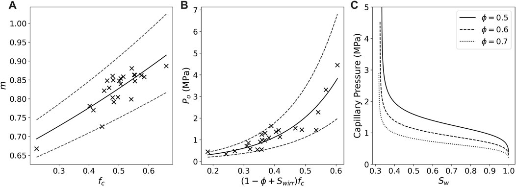
FIGURE 3. Best fit lines for van Genuchten parameters (A) m (Eq. 6) and (B) P_o (Eq. 7). Error bars of ±1 standard deviation are represented by gray dashed lines. Black X’s represent MICP measurements performed on marine sediments. (C) Water saturation graphed against capillary pressure for porosity ϕ =0.5 (solid line), ϕ =0.6 (dashed line), and ϕ =0.7 (dotted line).

The Peng and Robinson (1976) equation of state was used to calculate the pressure of methane gas based on temperature and the molar volume of the methane gas. We assumed values for methane critical temperature (T_c = 190.56 K), methane critical pressure (P_c = 45.99 bar), and methane acentric factor (ω = 0.011) based on Poling et al. (2001).

The relationship between gas pressure (u_g) and water pressure (u_w) is given by:

$u_g=u_w+u_c.(9)$

Using Eqs 2,5–9 and inputs of water depth, sediment depth, hydrate saturation, original temperature, and final temperature, we solved for capillary pressure using Newton-Raphson optimization. From the capillary pressure solution and the above equations, we were able to calculate final values for water pressure, gas pressure, methane molar volume, gas saturation, water saturation, and capillary pressure.

3.4.2 Undrained Model

In the undrained loading end member response to hydrate dissociation, methane and water mass are both conserved during the dissociation reaction. Thus, $mo{l}_{{\text{CH}}_4,i}$ = $mo{l}_{{\text{CH}}_4,f}$ and $mo{l}_{{\text{H}}_2\text{O},i}$ = $mo{l}_{{\text{H}}_2\text{O},f}$. To model undrained loading, we used a process similar to the drained loading model. In addition to Eqs 2,5–9, final water saturation (S_w,f) had to be considered as well as water density before and after hydrate dissociation. Water density was determined at a given temperature using the seawater equation of state of Safarov (2003):

$u_w=A{\rho }_w^2+B{\rho }_w^8+C{\rho }_w^{12}(10)$

where u_w has units MPa and ρ_w is in g/cm³. The coefficients A, B, C are polynomial functions of temperature (Safarov, 2003; Safarov et al., 2009).

In both the drained and undrained loading responses to hydrate dissociation, porosity was assumed constant. Thus, we were able to use the relation between hydrate and gas saturation from Daigle et al. (2020):

$S_h=S_g\frac{V_{m,h}}{V_{m,g}}(11)$

where the molar volume of gas is represented by V_m,g. We are assuming a structure I hydrate, so the molar volume of hydrate, represented by V_m,h, is a constant value: V_m,h = 132 cm³/mol. In a similar process to the drained loading method, final water pressure was calculated using Newton-Raphson optimization. We then calculated other values using Eqs 2,5–11.

3.4.3 Calculating Stresses

To calculate in situ stresses before hydrate dissociation, a simple calculation for hydrostatic water pressure was used:

$u_w=\left(z_{\mathit{water}}+z_{\mathit{sed}}\right){\rho }_{w}g(12)$

where z_water is water depth in meters, z_sed is depth below seafloor in meters, ρ_w = 1,024 kg/m³, g = 9.81 m/s², and u_w is in Pa. Overburden stress (σ_v) was determined by:

${\sigma }_v=z_{\mathit{water}}{\rho }_{w}g+g{\int }_0^{z_{\mathit{sed}}}{\rho }_b(13)$

where σ_v is in Pa. Bulk density (ρ_b) was determined at a given depth using the calculated porosity curve:

${\rho }_b=\varphi \left(z_{\mathit{sed}}\right){\rho }_w+\left(1-\varphi \left(z_{\mathit{sed}}\right)\right){\rho }_g(14)$

with a grain density ρ_g = 2,700 kg/m³.

Effective stress (σ′) prior to hydrate dissociation can be simply calculated as:

${\sigma }^{\prime }=\sigma -u_w.(15)$

Following the methods of Daigle et al. (2020), we assumed that the maximum principal stress is vertical (σ₁ = σ_v) and the sediments are vertically transversely isotropic (σ₂ = σ₃ = σ_h). The relation of ${\sigma }_h^{\prime }$ and ${\sigma }_v^{\prime }$ can be expressed as:

${\sigma }_h^{\prime }=\frac{\nu }{1-\nu }{\sigma }_v^{\prime }(16)$

or

${\sigma }_h=\frac{\nu }{1-\nu }\left({\sigma }_v-u_w\right)+u_w(17)$

where ν is Poisson’s ratio and subscripts v and h represent vertical and horizontal stresses respectively. To calculate Poisson’s ratio with depth, a sixth-order polynomial was fit to marine sediment data up to 650 m deep from Hamilton (1979).

$\begin{array}{ll}\hfill \nu \left(z\right)& =2.467\text{x}10^{-18}{z}^6-8.363\text{x}10^{-15}{z}^5+1.108\text{x}10^{-11}{z}^4-7.234\text{x}10^{-9}{z}^3\hfill \\ \hfill & +2.390\text{x}10^{-6}{z}^2-4.234\text{x}10^{-4}z+0.487.\hfill \end{array}(18)$

After dissociation, the pore space is a two-phase system of methane gas and water. To calculate effective stress, we followed the methods of Bishop (1959) and Nuth and Laloui (2008):

${\sigma }^{\prime }=\sigma -\pi (19)$

$\pi =S_w{u}_w+S_g{u}_g(20)$

where the equivalent pore pressure, π, is a weighted average of the water pressure and gas pressure in the system. Eqs 19,20 also hold for the pre-dissociation case with no gas pressure as u_g = 0 and thus π = u_w. With this, the change in effective stress at the BHZ due to hydrate dissociation was calculated.

3.4.4 Failure Model

A nonlinear Hoek-Brown failure envelope was constructed at each location with two goals in mind: 1. to determine if any failure occurred due to hydrate dissociation, and 2. which type of failure occurred (tensile or shear failure). This followed the work of Hoek and Brown (1997) and the methodology of Daigle et al. (2020). We assumed that the sediments were initially intact with no faults, fractures, or joints, so the tensile strength, T, was calculated by:

$T=\frac{c_u}{2}\left(m_i-\sqrt{m_i^2+4}\right)(21)$

where c_u is the unconfined compressive strength and m_i is the Hoek-Brown constant. We set m_i = 4 as reported by Hoek and Brown (1997) for claystones. This also follows the work done by Daigle et al. (2020) who note that m_i = 4 ± 2 is consistent with results from multiple triaxial shear experiments performed on marine muds and mudstones.

To calculate c_u, we used the correlation derived for muds and mudrocks by Ingram and Urai (1999):

${\log }_{10}{c}_u=-6.36+2.45{\log }_{10}\left(0.86V_{\text{p}}-1172\right)(22)$

where c_u is in MPa and V_p is the compressional wave velocity in m/s. At each depth we calculated V_p using the equation derived from Hamilton (1979) for marine sediments:

$V_{\text{p}}\left(z\right)=0.257z^3-0.741z^2+1.304z+1.511.(23)$

Finally, the Hoek-Brown failure envelope was calculated from Hoek and Brown (1997):

$\tau =A{c}_u{\left(\frac{{\sigma }_n^{\prime }-T}{c_u}\right)}^B,(24)$

where τ is the shear stress of the sample, ${\sigma }_n^{\prime }$ is the effective normal stress of the sample, and A and B are Hoek-Brown fitting parameters. Values of A = 1.02 and B = 0.858 were calculated by fitting failure envelopes to the results of triaxial tests performed on marine clays from the Gulf of Mexico and the Bay of Bengal (Silva et al., 2000; Moses et al., 2003; Dugan and Germaine, 2009).

The Hoek-Brown failure envelope was calculated based on the initial sediment properties prior to dissociation. Once dissociation occurred, both ${\sigma }_v^{\prime }$ and ${\sigma }_h^{\prime }$ were recalculated using Equation 19. Failure occurs if any points of the new Mohr circle lie to the left of the Hoek-Brown failure envelope. Since we assumed that the dissociation reaction went to completion, it was possible that the new effective stresses (${\sigma }_{v,f}^{\prime }$ and ${\sigma }_{h,f}^{\prime }$) both lie past the Hoek-Brown failure envelope. In reality, failure would initiate as soon as the Mohr circle began to cross the Hoek-Brown envelope: tensile failure occurring if the Mohr circle crossed the failure envelope at ${\sigma }_3^{\prime }=T$ (where ${\sigma }_3^{\prime }={\sigma }_h^{\prime }$) and shear failure occurring if the Mohr circle crossed the failure envelope when $|{\sigma }_3^{\prime }|<|T|$ (Figure 4).

FIGURE 4

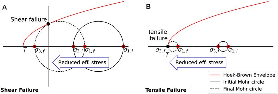
FIGURE 4. Example movement of Mohr circle due to hydrate dissociation. Initial stresses are denoted with the subscript i. Final stresses are denoted with the subscript f. In (A), shear failure occurs when the Mohr circle intersects the Hoek-Brown envelope at $|{\sigma }_3^{\prime }|<|T|$. In (B), tensile failure occurs when the Mohr circle intersects the Hoek-Brown envelope at $|{\sigma }_3^{\prime }|=|T|$.

4 Results

4.1 GPSM

The weight percent of TOC at the seafloor predicted with GPSM is shown in Figure 5 as well as the standard deviation and mean inexperience of these predictions. The highest TOC values were predicted along the line from (35.4°N, 75.0°W) to (39.0°N, 72.0°W). Comparing this region in the prediction map to the standard deviation map, known seafloor TOC values are sparse in this area and TOC standard deviations are higher than the rest of the predicted grid. The locations chosen along the shelf strike can be found in this area. The mean inexperience is calculated as the average distance in parameter space from the predicted location to its five nearest neighbors. Compared to the standard deviation map, a relatively low mean experience can be seen along the line from (35.4°N, 75.0°W) to (39.0°N, 72.0°W). Thus, although there is a high variance of predictions, there are other locations globally that are parametrically close to locations along this shelf strike line. A summary of the predicted weight percent of TOC for the nine modeled locations can be found in Table 3.

FIGURE 5

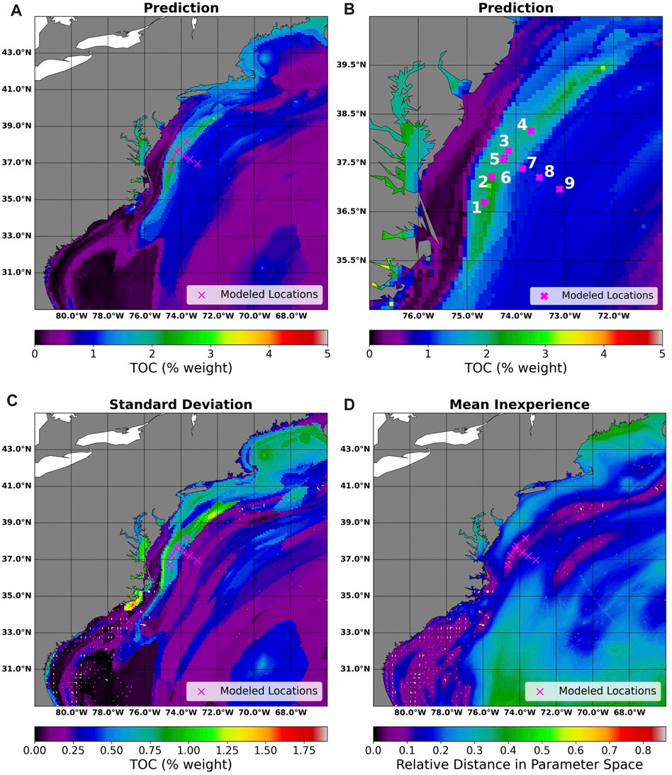
FIGURE 5. Output maps from GPSM over the area 29°N–45°N and 82°W–66°W. Plot (A) depicts the predicted weight percent of total organic carbon (TOC) on the seafloor. Plot (B) is the same mapped zoomed in around the area of interest with the locations modeled with PFLOTRAN/Dakota numbered. Between (35.4°N, 75.0°W) and (39.0°N, 72.0°W) an area of increased seafloor TOC was predicted. The locations along the shelf strike can be found in this area. Plots (C,D) show the standard deviation and mean inexperience of predictions over the region. Locations with known TOC values are marked by white dots on the standard deviation and mean inexperience maps. The nine locations where gas and hydrate formation was modeled are marked with a magenta ×.

TABLE 3

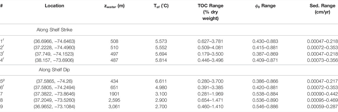
TABLE 3. Value ranges used in PLFOTRAN/Dakota model (gas locations^g and feather edge locations^f). For all locations, heat flux ranged from 42.3–52.2 mW/m².

4.2 Dakota and PFLOTRAN

The range of input values sampled by Dakota and used in the PFLOTRAN burial process to generate gas and hydrate are summarized in Table 3.

Average TOC predictions were around 2% dry weight at the shallower locations near the feather edge (sites 1–6). At deeper locations (sites 7–9), TOC predictions were closer to 1% dry weight. Seafloor porosity was around 65% at shallow locations and predictions increased to 73% for deeper location. Average sedimentation rates were just over 0.007 cm/yr with standard deviations around 0.1 cm/yr (Restreppo et al., 2020). As discussed in the Methods section, to avoid negative sedimentation rates, a lower bound for sedimentation rate was set at 3.16 × 10⁻⁵ cm/yr and any values sampled smaller than this value were set to 3.16 × 10⁻⁵ cm/yr. These sedimentation rates are lower than the sedimentation rates on the U.S. Atlantic margin found to the north and south, but the studied location could simply be in an area of low sediment influx. Measurements to the north along the U.S. Atlantic margin (offshore of New Jersey) range from 0.011 cm/yr to 0.058 cm/yr (Shipboard Scientific Party, 1994a; Shipboard Scientific Party, 1994b; Shipboard Scientific Party, 1994c; Shipboard Scientific Party, 1994d; Shipboard Scientific Party, 1994e; Shipboard Scientific Party, 1998a) while locations to the south (offshore North Carolina) are closer to 0.02 cm/yr (Shipboard Scientific Party, 1994b; Shipboard Scientific Party, 1994c; Shipboard Scientific Party, 1996a; Shipboard Scientific Party, 1998b). Location nine had a much lower predicted sedimentation rate than the other eight locations, corresponding to its further distance from the shelf edge and seacoast, as well as its overall depth. Heat flux for all simulations were between 42.3 and 52.2 mW/m².

At each location, we ran 50 simulations using PFLOTRAN, and sampled the seafloor TOC, seafloor porosity, sedimentation rate, and heat flux inputs with Dakota. For an individual location, the resulting output profiles of gas, hydrate, and temperature were plotted against depth, and a base of hydrate stability was calculated. Figure 6 shows the hydrate saturation profiles and the gas saturation profiles with depth for the nine study locations.

FIGURE 6

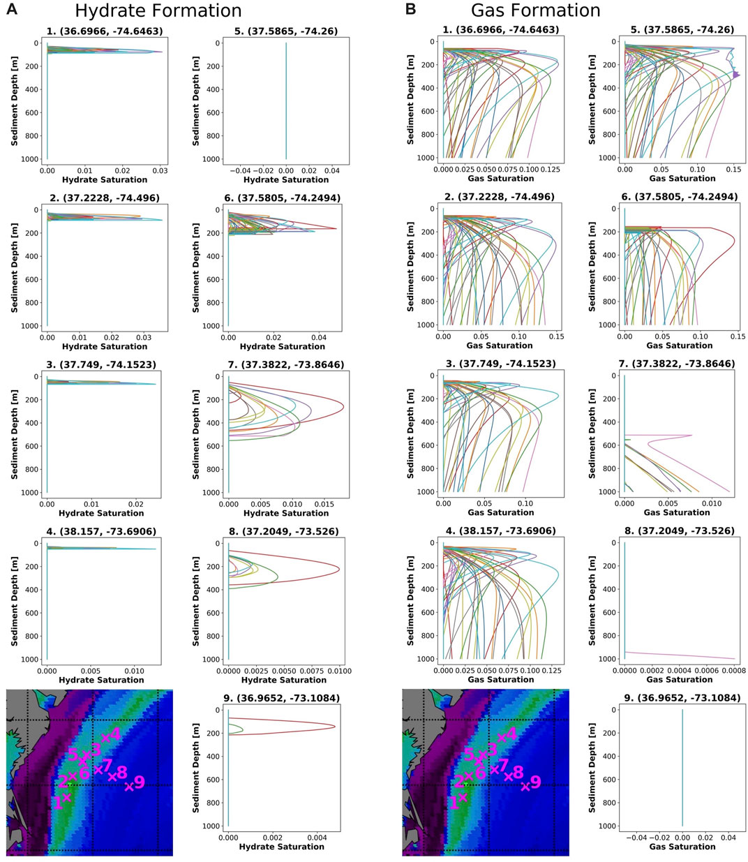
FIGURE 6. Figure (A) shows simulation outputs of hydrate saturation with depth at each modeled location. Figure (B) shows simulation outputs of gas saturation with depth at each modeled location.

Figure 7 shows an example temperature profile with depth for site 1, and includes the hydrate phase envelope calculated from Kamath (1984):

$P=\exp \left[38.980-\frac{8533.80}{T}\right](25)$

where hydrostatic pressure, P (kPa), can be calculated at a given sediment depth using Eq. 12, allowing us to calculate temperature, T (K). The phase envelope was included to illustrate the difference in the BHZ between simulations. Due to the diversity of sampled heat flux values, the geothermal gradient for each simulation is different, leading to a range of depths where the phase envelope is crossed and thus a range of BHZ depths.

FIGURE 7

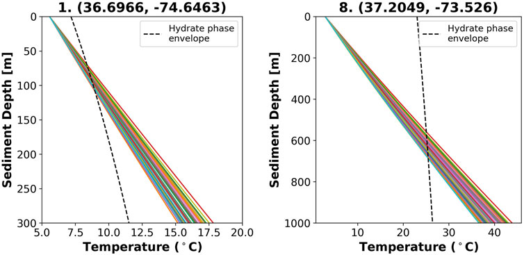
FIGURE 7. Temperature with depth at Site 1 (36.6966, −74.6463) and Site 8 (37.2049, −73.5260). Hydrates are stable where the temperature profile is to the left of the hydrate phase envelope (black dashed line). Around 80 mbsf sediment depth at Site 1 (water depth 508 m), temperature profiles begin to cross the hydrate phase envelope, so hydrate is no longer stable. At the deeper Site 8 (water depth 2,595 m), temperature profiles begin to cross the hydrate phase envelope around 550 mbsf. Note the different depth scales between the two temperature profiles. This was done to better visualize the intersection of the phase envelope at Site 1.

Table 4 summarizes the hydrate profiles shown in Figure 6. Some simulations failed to run or ran into oscillatory errors, thus producing no hydrate or gas predictions. The number of runs that produced hydrate and gas profiles (successful runs) is noted at each location. In addition, the number of runs where hydrate formed is summarized. At each site, the average BHZ was calculated as the depth where the hydrate phase envelope from Kamath (1984) intersected the average temperature profile at the location. In addition, we noted the maximum depth at which hydrate formed (Max hyd. depth) at each location. This depth represents the extent of the zone of actual hydrate occurrence where the concentration of methane exceeds the solubility of methane in seawater in addition to the pressure and temperature conditions of the hydrate stability zone (Xu and Ruppel, 1999). At sites 1-4 and site 6, the average extent of the zone of hydrate occurrence is very similar the calculated BHZ. Looking at the profiles for these five locations, hydrate concentrations are often at a maximum at this depth before they drop to zero and methane gas is witnessed instead. The minimum and maximum extent of the zone of hydrate occurrence are also noted, illustrating the varying extent of the BHZ between models as shown in Figure 7.

TABLE 4

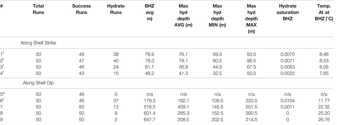
TABLE 4. Summary of hydrate profiles modeled with PFLOTRAN and Dakota (gas locations^g and feather edge locations^f).

At sites 7-9, fewer simulations result in the growth of hydrate. As was done for sites 1-4 and 6, the average depth of the BHZ was calculated for these sites. Interestingly, at these deeper locations, the average extent of the zone of hydrate occurrence was much shallower than the depth of the BHZ. At site 7, the average BHZ is 516.5 mbsf, although graphically it can be seen that a majority of the hydrate profiles do not reach this depth (Figure 6). Even fewer simulations form hydrate at sites 8 and 9, and none of the simulations produce hydrate near the depth of the BHZ (601.4 mbsf and 647.7 mbsf respectively) at these locations. In profile 5, no hydrate forms. This location is upslope of the feather edge and outside of the hydrate stability zone.

A distribution of total hydrate mass for each profile is shown in Figure 8. Site 6 has the largest distribution of total hydrate formed, however site 7 has the largest amounts of hydrate formed in a run. The larger values of hydrate mass in sites 7-9 can be attributed to the thickness of the hydrate stability zone at these locations. Near the feather edge (sites 1–4) many runs do not generate hydrate, and those that do have very thin hydrate layers due to the shallow BHZ. This leads to much lower predictions of total hydrate formed in this area.

FIGURE 8

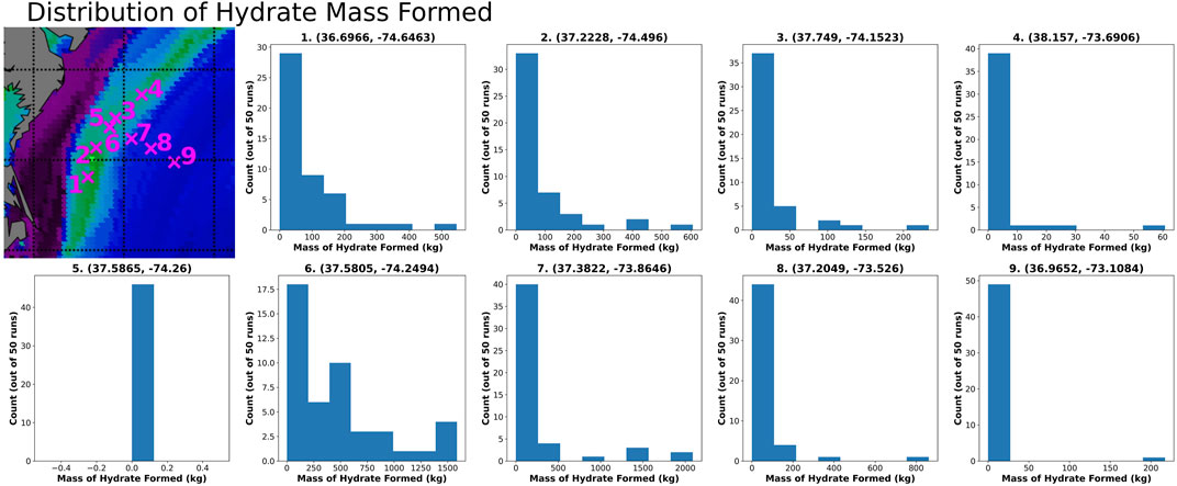
FIGURE 8. Distribution of the mass of hydrate formed at each location.

The gas saturation profiles shown in Figure 6 are summarized in Table 5. Gas generation occurs within the modeled 1,000 m sediment column in eight of the simulations. The only simulation in which no gas was generated during the 50 runs was at the deepest location, site 9. When calculating the maximum gas saturation and the depth of the maximum gas saturation in Table 5, only maximum saturations shallower than 1,000 m were considered. Therefore, site eight does not have a maximum gas saturation value or depth. The maximum gas saturation for site seven occurs in only one run and may be an outlier. Comparing the remaining six locations, site 5 has the largest average maximum gas saturation. As discussed, this site is upslope of the feather edge and outside of the hydrate stability zone.

TABLE 5

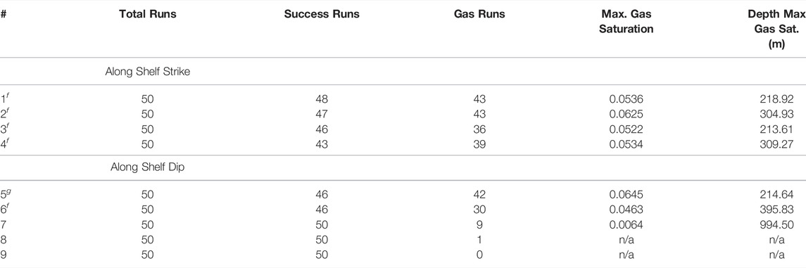
TABLE 5. Summary of gas profiles modeled with PFLOTRAN and Dakota (gas locations^g and feather edge locations^f).

4.3 Dissociation and Failure Criteria

At the five locations along the feather edge (sites 1–4, 6) we modeled hydrate dissociation at the BHZ due to a temperature increase of 1°C, ignoring any changes in pressure over time due to the rise and fall of sea level were ignored. At each location, we calculated a final gas saturation due to dissociation, along with the resulting final water pressure, final gas pressure, and capillary pressure (Table 6). A value for π (Eq. 20) was also calculated at each location. Comparing the drained and undrained models, both predict a decrease from the initial saturation of hydrate to the final saturation of gas. This is because a constant density (and thus molar volume) was chosen for hydrate whereas the methane gas that forms is compressible. Although the BHZ at these locations is relatively near the seafloor, there is still enough pressure from the 50–100 m of sediment and 500 m of water to compress any gas that forms. In the drained model, hydrate saturation decreases to the final gas saturation by a factor of about four ($\frac{1}{4}$S_h ≈ S_g). In the undrained model, the decrease in hydrate saturation to gas saturation is over twice as large ($\frac{1}{10}$S_h ≈ S_g). In the undrained environment water pressure is not held constant during dissociation and instead the total moles of water before and after dissociation is constant, leading to a larger decrease in hydrate to gas saturation. The impact of drainage can also be seen when comparing the water pressures calculated before (u_w,i) and after (u_w,f) dissociation for both models. By definition, the drained model has a constant water pressure during hydrate dissociation. This leads to final gas pressures (u_g,f) that are similar to the water pressure. On the other hand, when hydrate dissociates in the undrained model, water pressure nearly doubles at every location. Capillary pressure (u_c) in the undrained model is similar to capillary pressure in the drained model, however the large increase in water pressure leads to a higher final gas pressure and higher π value (Eq. 20).

TABLE 6

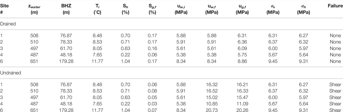
TABLE 6. Geomechanical Model: Pressures and stresses due to hydrate dissociation along the shelf edge. An increase in temperature by 1 °C was used to initiate dissociation for both the drained and undrained models.

At each location, the total horizontal and vertical stresses and the effective horizontal and vertical stresses were calculated before and after hydrate dissociation (Table 6). Total stresses were relatively consistent among the five locations as they all lie along the shelf strike. During dissociation, the effective stress on the sediment decreases (${\sigma }_{v,f}^{\prime }<{\sigma }_{v,i}^{\prime }$ and ${\sigma }_{h,f}^{\prime }<{\sigma }_{h,i}^{\prime }$). In the drained environment, no failure was modeled at any location as the representative Mohr circle never crosses the Hoek-Brown failure envelope during the hydrate dissociation. In the undrained system, the effective vertical and horizontal stresses decrease to the point where the representative Mohr circle intersects with the Hoek-Brown failure envelope. At each location this occurred when $|{\sigma }_3^{\prime }|<|T|$ so we expect shear failure.

5 Discussion

5.1 GPSM

Our predictive map of seafloor TOC from GPSM was comparable to the work done by Lee et al. (2019) and Eymold et al. (2021). The global map of seafloor TOC produced by Lee et al. (2019) also predicted an area of increased TOC off the east coast of the United States in the same region [(35.4°N, 75.0°W) to (39.0°N, 72.0°W)] predicted in our model. The map of seafloor TOC predicted by Eymold et al. (2021) covers about a quarter of the area of our prediction. In this prediction, trends of TOC are similar to the trends we predict as Eymold et al. (2021) also predicts an increase in TOC at the southern end of the (35.4°N, 75.0°W) to (39.0°N, 72.0°W) region. It is unsurprising that the areas with increased TOC predictions are similar between this work and the work done by Lee et al. (2019) and Eymold et al. (2021). Although the data sets used between the three predictions differed slightly, the general methodology was consistent across the models.

To ensure the accuracy of our seafloor TOC model, it is additionally important to compare the results to field data in the area. Investigations by Skarke et al. (2014) have found multiple instances of methane gas leakage from the seafloor along the U.S. Atlantic margin in the form of gas plumes (Figure 9). The sites of these methane seeps correspond with areas predicted by our GPSM model to have higher values of seafloor TOC, specifically in the region between (35.4°N, 75.0°W) and (39.0°N, 72.0°W). The seeps identified by Skarke et al. (2014) are mostly found just updip of the feather edge. At these locations, seepage is most likely due to small tensile failures that occur when microbial gas is generated close to the seafloor (Daigle et al., 2020). However, at the feather edge where we modeled hydrate and gas formation with PFLOTRAN/Dakota, if hydrate dissociates it will instead cause shear failure.

FIGURE 9

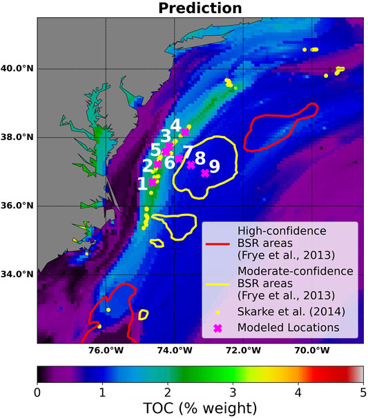
FIGURE 9. Output maps from GPSM over the area 32°N–41.5°N and 78°W–68.5°W. Methane seeps (yellow dots) identified by Skarke et al. (2014) are also plotted and support the increased TOC prediction between (35.4°N, 75.0°W) and (39.0°N, 72.0°W). Locations where we modeled hydrate and gas formation are marked with a magenta × and numbered. Red and yellow outlines are areas where the U.S. Bureau of Ocean Energy Management (BOEM) identified BSRs in seismic data (Frye et al., 2013).

Around the U.S. Atlantic margin, the U.S. Bureau of Ocean Energy Management (BOEM) identified six unique regions with BSRs of moderate and high confidence (Frye et al., 2013). Some of these regions with identified BSRs overlay the region where we predicted high TOC values and modeled hydrate and gas formation. Our model forms hydrate and gas through methanogenesis and therefore suggests that the BSRs identified by Frye et al. (2013) may have a similar local microbial origin and that the concentration of gas and hydrate in the pore space may be small.

5.2 Hydrate and Gas Formation

When using PFLOTRAN, a 120,000 years time period corresponding to the length of a glacial-interglacial cycle was chosen to simulate methanogenesis and hydrate formation. This gave us a good idea of hydrate profiles along the feather edge of hydrate stability, and we demonstrated that conditions exist in which failure will occur due to dissociation. If we instead wanted to model the actual burial history and hydrate formation in this area, we would need to include changes in temperature, pressure, and sedimentation rate over time. However, even though gas seeps (Skarke et al., 2014) and regions with BSRs of moderate to high confidence (Frye et al., 2013) have been identified in the area we are modeling (Figure 9), there are still few constraints on the distribution and amount of gas and hydrate in the area. Therefore, we chose to model a variety of outcomes using Dakota to sample different initial seafloor conditions.

Once the hydrate/gas profile has been put in place we assumed an increase in temperature on a time scale much shorter than 120,000 years. One cause of this temperature change could be a weakened Atlantic Meridional Overturning Circulation (AMOC) which could lead to increased surface and seafloor temperatures in our area of interest (Liu et al., 2020; Garcia-Soto et al., 2021). The movement of the feather edge due to changes in seafloor temperature has also been shown on a shorter timescale by Phrampus and Hornbach (2012) just south of the region we modeled. Changes in sea level can also alter the GHSZ as pressure changes as the seafloor. Not only can changes in sea level shift the feather edge, but lower past sea levels can create an area within the current GHSZ where hydrate was unable to accumulate over time (Stranne et al., 2016).

In the area of study, varying sedimentation rates over the Pleistocene are noted by McHugh and Olson (2002). Since our model relies on sedimentation to transport organic matter, it would seem that given identical TOC measurements, the sedimentation rate would increase the amount of methane hydrate and gas formed in the simulation. This is discussed by Eymold et al. (2021) who concur that as the sedimentation rate approaches zero, hydrate growth is unexpected. Eymold et al. (2021) also note that increasing sedimentation rate in their experience can eventually lead to reduced hydrate growth as the organic carbon is buried so quickly it cannot go through the methanogenesis process. In reality, changing sedimentation rates over time will affect the concentration of TOC on the ocean floor. In the area we model, organic matter on the seafloor is mainly marine-driven with only a little mixing of terrestrial material (Shipboard Scientific Party, 1994a; Shipboard Scientific Party, 1994b; Shipboard Scientific Party, 1994c; Shipboard Scientific Party, 1994d; Shipboard Scientific Party, 1994e). Higher sedimentation rates in the area would lead to a larger flux of terrestrial organic to the seafloor, however there would also be more sediment deposited relative to the standard background flux of marine organic carbon. Therefore, a variable sedimentation rate over time would have to consider the changing seafloor TOC concentrations and may still result in predictions similar to models where seafloor TOC and sedimentation rates are held constant.

Sampling methanogenesis rate in the PFLOTRAN/Dakota model also changes the outcomes of the simulations. Since we do not know the exact methanogenesis rate in the area or the probability distribution of the methanogenesis rate, we chose a constant value within the range modeled by Eymold et al. (2021) and also between the values of λ estimated by Bhatnagar et al. (2007) and Malinverno (2010). The effect of changing methanogenesis rate in the model is discussed by Eymold et al. (2021) who found that higher methanogenesis rates led to a deeper BHZ but a lower maximum hydrate saturation. We have included additional hydrate and gas profiles in the supplementary materials where we sampled methanogenesis rate in addition to the other previously sampled parameters.

5.3 Sediment Failure Model

In all five locations along the feather edge (sites 1–4, 6) shear failure occurred in the undrained model while no shear failure occurred in the drained model. At these sites, the largest average saturation of hydrate at the BHZ was predicted to be 1% (site 6). At the other four sites, the average predicted hydrate saturation at the BHZ was at or below 0.7%. At these locations gas saturation after dissociation was no more than 0.2%. In the undrained environment, gas saturations formed from dissociation were below 0.1%. Even with these relatively low saturations of gas formed from dissociation, hydrate dissociation under undrained conditions led to shear failure. This differs from the conclusion of Daigle et al. (2020) who suggest that tensile fracturing is generally favored in the shallowest sediments near the feather edge. The BHZ modeled in this paper with PFLOTRAN is at depths between 40 and 80 m (along with site 6 at 182 m). Thus, the sediments modeled may still be too deep below the seafloor to experience gas-driven tensile fracturing.

In the undrained model, shear failure occurs due to increased pore pressure and gas pressure in the sediment. As pore pressure increases, the effective stress decreases to the point where the sediment enters a failure regime. As depicted in Figure 4, this can be visualized as the Mohr circle shifting to the left until it intersects with the Hoek-Brown failure envelope. Due to the depths of our modeled BHZ, the representative Mohr circle intersected with Hoek-Brown failure envelope at $|{\sigma }_3^{\prime }|<|T|$. Closer to the seafloor the stresses are nearly isotropic, and the representative Mohr circle could be small enough that a decrease in effective stress leads to tensile failure when $|{\sigma }_3^{\prime }|=|T|$. Stranne et al. (2017) note that fractures will not occur near the feather edge in sediments with permeabilities larger than 10^–15 m². Although we use a permeability value of 10^–15 m² in our burial model to account for siltier beds, multiple ODP wells (sites 902, 903, and 1,073) in the region describe permeabilities between 10^–17 and 10^–16 m² (Blum et al., 1996; Dugan et al., 2003), so shear failure still may occur due to hydrate dissociation.

The low saturation of gas formed from hydrate dissociation needed for the dissociation to cause shear failure has interesting implications on slope stability for the region. Looking at the area of high TOC values predicted with GPSM that overlap with the methane seepage locations highlighted by Skarke et al. (2014), there is a 250 km region along the continental slope where high TOC values are expected (and where methane seeps have already been found). Even with low hydrate concentrations between 0.2% and 1%, if this hydrate dissociates in an undrained environment, shear failure could ensue. In reality, the drainage environment will be somewhere between the drained and undrained endmembers. Therefore, it will eventually be important to have a mixed-drainage model to determine the possibility of failure due to hydrate dissociation in a region. In addition, it will be important to look at hydrate dissociation as a step by step process where local pressure change during dissociation can cause hydrate to reform. When considering this, the rate at which temperature changes and the rate of fluid flow are important in correctly modeling the grain space.

For slope failure or submarine landslides to occur in an area, there needs to be some sort of triggering mechanism such as an earthquake, changing sea level, or high internal pore pressure causing the downslope component of stress to become larger than the resisting stress (Hampton et al., 1996). The dissociation of methane hydrate has also been found to lead to shear failure in seafloor sediments resulting in seafloor slumping and submarine landslides (Kvenvolden, 1993; Hampton et al., 1996; Hornbach et al., 2007; Elger et al., 2018). The timing of slope failure due to hydrate dissociation has been investigated by Lee (2009), Maslin et al. (2004), and Nixon and Grozic (2007), who have shown possible connections globally between hydrate dissociation and submarine landslides. The mechanism by which hydrate dissociation leads to slope instability has been discussed as well. In both fine grained and coarse grained sediments, fluid migration towards the seafloor can occur along active thrust faults leading to a build up of gas pressure, resulting in lower effective stresses and sediment instability (Conti et al., 2008; Argentino et al., 2019). In areas without thrust faults to act as a conduit for gas migration, Kvenvolden (1993) suggests that the dissociation of hydrates can create an “enhanced fluidized layer” beneath the GHSZ, leading to the slope failure. Elger et al. (2018) suggest that the overpressure of gas at the BHZ creates a gas pipe to shallower sediments, and it is in these shallower coarse-grained sediments where gas builds up, leading to shear failure.

A factor of safety calculation, containing the seafloor slope variable, compares resisting to shearing forces in a sediment and can be used to determine if slope failure is likely to occur at a submarine location (Løseth, 1999; ten Brink et al., 2009). Along the U.S. Atlantic continental slope most submarine landslides originate from areas with a seafloor slope angle between 2 and 4°(Booth et al., 1993). In the area of our study, the gradient of the continental slope is mostly between 4 and 8 with some areas reaching 8–12°(Twichell et al., 2009) thus slope failure may be a concern under the undrained conditions that we modeled.

6 Conclusion

We used a geospatial machine learning model to create a global map of TOC on the seafloor. Focusing specifically on the U.S. Atlantic margin, the region with high TOC predictions between (35.4°N, 75.0°W) and (39.0°N, 72.0°W) was consistent with methane gas seeps located by Skarke et al. (2014). We then modeled hydrate and gas formation over a 120,000 years time period at nine locations in this area: five hydrate bearing locations along the feather edge, one gas location updip of the feather edge, and three hydrate bearing locations downdip of the feather edge. For each of these locations, hydrate and gas formation were modeled by sampling seafloor TOC, seafloor porosity, sedimentation rate, and heat flux.

At the feather edge, we modeled hydrate dissociation at the BHZ due to an increase in temperature while ignoring the change in pressure due to the rise and fall of sea level. In a purely drained environment, no failure is expected to occur due to hydrate dissociation. However, in an undrained environment, the criterion for shear failure is quickly met during hydrate dissociation. Even as gas saturations due to hydrate dissociation stayed below 0.1% (hydrate saturations: 0.2%—1%) shear failure was predicted to occur. This suggests that the hydrate that forms over one glacial cycle can cause submarine slope failure upon dissociation.

Data Availability Statement

The raw data supporting the conclusion of this article will be made available by the authors, without undue reservation.

Author Contributions

OC performed the numerical modeling and wrote the manuscript. HD supervised the project and edited the manuscript. Both authors read and approved the final manuscript.

Funding

This work was supported by the University of Texas at Austin, and the Laboratory Directed Research and Development program at Sandia National Laboratories. Sandia National Laboratories is a multimission laboratory managed and operated by National Technology and Engineering Solutions of Sandia, LLC., a wholly owned subsidiary of Honeywell International, Inc., for the U.S. Department of Energy’s National Nuclear Security Administration under contract DE-NA-0003525.

Conflict of Interest

The authors declare that the research was conducted in the absence of any commercial or financial relationships that could be construed as a potential conflict of interest.

Publisher’s Note

All claims expressed in this article are solely those of the authors and do not necessarily represent those of their affiliated organizations, or those of the publisher, the editors and the reviewers. Any product that may be evaluated in this article, or claim that may be made by its manufacturer, is not guaranteed or endorsed by the publisher.

Acknowledgments

The authors thank Ali Shirani Lapari and Mitchel Broten for preliminary machine learning work. Constructive comments from CS, DF, and Editor AL helped strengthen this paper.

Supplementary Material

The Supplementary Material for this article can be found online at: https://www.frontiersin.org/articles/10.3389/feart.2022.835685/full#supplementary-material

References

Adams, B. M., Bohnhoff, W. J., Dalbey, K. R., Ebeida, M. S., Eddy, J. P., Eldred, M. S., et al. (2021). enDakota, A Multilevel Parallel Object-Oriented Framework for Design Optimization, Parameter Estimation, Uncertainty Quantification, and Sensitivity Analysis: Version 6.14. User’s Man. 354. doi:10.2172/1784843

CrossRef Full Text | Google Scholar

Argentino, C., Conti, S., Crutchley, G. J., Fioroni, C., Fontana, D., and Johnson, J. E. (2019). Methane-derived Authigenic Carbonates on Accretionary Ridges: Miocene Case Studies in the Northern Apennines (Italy) Compared with Modern Submarine Counterparts. Mar. Petroleum Geol. 102, 860–872. doi:10.1016/j.marpetgeo.2019.01.026

CrossRef Full Text | Google Scholar

Bhatnagar, G., Chapman, W. G., Dickens, G. R., Dugan, B., and Hirasaki, G. J. (2007). Generalization of Gas Hydrate Distribution and Saturation in Marine Sediments by Scaling of Thermodynamic and Transport Processes. Am. J. Sci. 307, 861–900. doi:10.2475/06.2007.01

CrossRef Full Text | Google Scholar

Biastoch, A., Treude, T., Rüpke, L. H., Riebesell, U., Roth, C., Burwicz, E. B., et al. (2011). enRising Arctic Ocean Temperatures Cause Gas Hydrate Destabilization and Ocean Acidification. Geophys. Res. Lett. 38. doi:10.1029/2011gl047222

CrossRef Full Text | Google Scholar

Bishop, A. W. (1959). The Principle of Effective Stress. Tek. Ukebl. 39, 859–863.

Google Scholar

Blum, P., Xu, J., and Donthireddy, S. (1996). enGeotechnical Properties of Pleistocene Sediments from the New Jersey Upper Continental Slopeof Proceedings of the Ocean Drilling Program. Sci. Results Ocean. Drill. Program. 150. doi:10.2973/odp.proc.sr.150.1996

CrossRef Full Text | Google Scholar

Booth, J. S., O’Leary, D. W., Popenoe, P., and Danforth, W. W. (19932002). “US Atlantic Continental Slope Landslides: Their Distribution, General Attributes, and Implications,” in Submarine Landslides: Selected Studies in the US Exclusive Economic Zone (U.S. Geol. Surv. Bull.), 14–22.

Google Scholar

Boudreau, B. P. (2012). The Physics of Bubbles in Surficial, Soft, Cohesive Sediments. Mar. Petroleum Geol. 38, 1–18. doi:10.1016/j.marpetgeo.2012.07.002

CrossRef Full Text | Google Scholar

Boyer, T. P., Baranova, O. K., Coleman, C., Garcia, H. E., Grodsky, A., Locarnini, R. A., et al. (2018). enWorld Ocean Database, 2018, 207.

Google Scholar

Brothers, D. S., Ruppel, C., Kluesner, J. W., ten Brink, U. S., Chaytor, J. D., and Hill, J. C. (2014). enSeabed Fluid Expulsion along the Upper Slope and Outer Shelf of the U.S. Atlantic Continental Margin. Geophys. Res. Lett. 41, 96–101. doi:10.1002/2013GL058048

CrossRef Full Text | Google Scholar

Cathles, L. M., Su, Z., and Chen, D. (2010). enThe Physics of Gas Chimney and Pockmark Formation, with Implications for Assessment of Seafloor Hazards and Gas Sequestration. Mar. Petroleum Geol. 27, 82–91. doi:10.1016/j.marpetgeo.2009.09.010

CrossRef Full Text | Google Scholar

Conti, S., Fontana, D., and Lucente, C. (2008). enAuthigenic Seep-Carbonates Cementing Coarse-Grained Deposits in a Fan-Delta Depositional System (Middle Miocene, Marnoso-Arenacea Formation, Central Italy). Sedimentology 55, 471–486. doi:10.1111/j.1365-3091.2007.00910.x

CrossRef Full Text | Google Scholar

Daigle, H., Cook, A., Fang, Y., Bihani, A., Song, W., and Flemings, P. B. (2020). enGas-Driven Tensile Fracturing in Shallow Marine Sediments. J. Geophys. Res. Solid Earth 125. doi:10.1029/2020JB020835

CrossRef Full Text | Google Scholar

Daigle, H., Ghanbarian, B., Henry, P., and Conin, M. (2015). enUniversal Scaling of the Formation Factor in Clays: Example from the Nankai Trough. J. Geophys. Res. Solid Earth 120, 7361–7375. doi:10.1002/2015JB012262

CrossRef Full Text | Google Scholar

Dickens, G. R., Paull, C. K., and Wallace, P. (1997). enDirect Measurement of In Situ Methane Quantities in a Large Gas-Hydrate Reservoir. Nature 385, 426–428. doi:10.1038/385426a0

CrossRef Full Text | Google Scholar

Dugan, B., and Germaine, J. T. (2009). Data Report: Strength Characteristics of Sediments from IODP Expedition 308, Sites U1322 and U1324. Proc. Integr. Ocean Drill. Program 308, 1–13. doi:10.2204/iodp.proc.308.210.2009

CrossRef Full Text | Google Scholar

Dugan, B., Olgaard, D. L., Flemings, P. B., and Gooch, M. (2003). enData Report: Bulk Physical Properties of Sediments from ODP Site 1073, Vol. 174A of Proceedings of the Ocean Drilling Program. Sci. Results Ocean. Drill. Program. doi:10.2973/odp.proc.sr.174A.2003

CrossRef Full Text | Google Scholar

Egger, M., Riedinger, N., Mogollón, J. M., and Jørgensen, B. B. (2018). enGlobal Diffusive Fluxes of Methane in Marine Sediments. Nat. Geosci. 11, 421–425. doi:10.1038/s41561-018-0122-8

CrossRef Full Text | Google Scholar

Elger, J., Berndt, C., Rüpke, L., Krastel, S., Gross, F., and Geissler, W. H. (2018). enSubmarine Slope Failures Due to Pipe Structure Formation. Nat. Commun. 9, 715. doi:10.1038/s41467-018-03176-1

PubMed Abstract | CrossRef Full Text | Google Scholar

Eymold, W. K., Frederick, J. M., Nole, M., Phrampus, B. J., and Wood, W. T. (2021). enPrediction of Gas Hydrate Formation at Blake Ridge Using Machine Learning and Probabilistic Reservoir Simulation. Geochem. Geophys. Geosystems 22. doi:10.1029/2020GC009574

CrossRef Full Text | Google Scholar

Ferré, B., Mienert, J., and Feseker, T. (2012). enOcean Temperature Variability for the Past 60 Years on the Norwegian-Svalbard Margin Influences Gas Hydrate Stability on Human Time Scales. J. Geophys. Res. Oceans 117. doi:10.1029/2012JC008300._eprint

CrossRef Full Text | Google Scholar

Fleischer, P., Orsi, T. H., Richardson, M. D., and Anderson, A. L. (2001). enDistribution of Free Gas in Marine Sediments: a Global Overview. Geo-Marine Lett. 21, 103–122. doi:10.1007/s003670100072

CrossRef Full Text | Google Scholar

Frye, M., Shedd, W., and Schuenemeyer, J. (2013). Gas Hydrate Resource Assessment: Atlantic Outer Continental Shelf. Washington, D.C: U.S. Bureau of Ocean Energy Management. Technical Report RED 2013-01.

Google Scholar

Fuchs, S., Norden, B., and Commission, I. H. F. (2021). enThe Global Heat Flow Database: Release 2021 GFZ Data Services.

Google Scholar

Garcia-Soto, C., Cheng, L., Caesar, L., Schmidtko, S., Jewett, E. B., Cheripka, A., et al. (2021). An Overview of Ocean Climate Change Indicators: Sea Surface Temperature, Ocean Heat Content, Ocean pH, Dissolved Oxygen Concentration, Arctic Sea Ice Extent, Thickness and Volume, Sea Level and Strength of the AMOC (Atlantic Meridional Overturning Circulation). Front. Mar. Sci. 8. doi:10.3389/fmars.2021.642372

CrossRef Full Text | Google Scholar

Graw, J. H., Wood, W. T., and Phrampus, B. J. (2021). enPredicting Global Marine Sediment Density Using the Random Forest Regressor Machine Learning Algorithm. J. Geophys. Res. Solid Earth 126, e2020JB020135. doi:10.1029/2020JB020135

CrossRef Full Text | Google Scholar

Hamilton, E. L. (1979). enV_p/V_s and Poisson’s Ratios in Marine Sediments and Rocks. J. Acoust. Soc. Am. 66, 1093–1101. doi:10.1121/1.383344

CrossRef Full Text | Google Scholar

Hammond, G. E., Lichtner, P. C., and Mills, R. T. (2014). enEvaluating the Performance of Parallel Subsurface Simulators: An Illustrative Example with PFLOTRAN. Water Resour. Res. 50, 208–228. doi:10.1002/2012WR013483

PubMed Abstract | CrossRef Full Text | Google Scholar

Hampton, M. A., Lee, H. J., and Locat, J. (1996). enSubmarine Landslides. Rev. Geophys. 34, 33–59. doi:10.1029/95rg03287

CrossRef Full Text | Google Scholar

Hill, J. C., Driscoll, N. W., Weissel, J. K., and Goff, J. A. (2004). enLarge-Scale Elongated Gas Blowouts along the U.S. Atlantic Margin. J. Geophys. Res. Solid Earth 109. doi:10.1029/2004JB002969

CrossRef Full Text | Google Scholar

Hoek, E., and Brown, E. T. (1997). enPractical Estimates of Rock Mass Strength. Int. J. Rock Mech. Min. Sci. 34, 1165–1186. doi:10.1016/S1365-1609(97)80069-X

CrossRef Full Text | Google Scholar

Holbrook, W. S., Hoskins, H., Wood, W. T., Stephen, R. A., and Lizarralde, D. (1996). Leg 164 Science Party enMethane Hydrate and Free Gas on the Blake Ridge from Vertical Seismic Profiling. Science 273, 1840–1843. doi:10.1126/science.273.5283.1840

CrossRef Full Text | Google Scholar

Hornbach, M. J., Lavier, L. L., and Ruppel, C. D. (2007). enTriggering Mechanism and Tsunamogenic Potential of the Cape Fear Slide Complex, U.S. Atlantic Margin. Geochem. Geophys. Geosystems 8. doi:10.1029/2007GC001722

CrossRef Full Text | Google Scholar

Ingram, G. M., and Urai, J. L. (1999). enTop-Seal Leakage through Faults and Fractures: the Role of Mudrock Properties. Geol. Soc. Lond. Spec. Publ. 158, 125–135. doi:10.1144/GSL.SP.1999.158.01.10

CrossRef Full Text | Google Scholar

Johnson, B. D., Barry, M. A., Boudreau, B. P., Jumars, P. A., and Dorgan, K. M. (2012). enIn Situ Tensile Fracture Toughness of Surficial Cohesive Marine Sediments. Geo-Marine Lett. 32, 39–48. doi:10.1007/s00367-011-0243-1

CrossRef Full Text | Google Scholar

Judd, A. G. (2003). enThe Global Importance and Context of Methane Escape from the Seabed. Geo-Marine Lett. 23, 147–154. doi:10.1007/s00367-003-0136-z

CrossRef Full Text | Google Scholar

Kamath, V. A. (1984). EnglishStudy of Heat Transfer Characteristics during Dissociation of Gas Hydrates in Porous Media. United States – Pennsylvania: Ph.D., University of Pittsburgh.

Google Scholar

Kominz, M. A., Patterson, K., and Odette, D. (2011). Lithology Dependence of Porosity in Slope and Deep Marine Sediments. J. Sediment. Res. 81, 730–742. doi:10.2110/jsr.2011.60

CrossRef Full Text | Google Scholar

Kvenvolden, K. A., and Claypool, G. E. (1988). “Gas Hydrates in Oceanic Sediment,” in Tech. Rep.U.S. Geological Survey (Publication Title: Open-File Report), 88–216. ISSN: 2331-1258. doi:10.3133/ofr88216

CrossRef Full Text | Google Scholar

Kvenvolden, K. A. (1993). enGas Hydrates—Geological Perspective and Global Change. Rev. Geophys. 31, 173–187. doi:10.1029/93RG00268

CrossRef Full Text | Google Scholar

Kvenvolden, K. A., and Lorenson, T. D. (2001). “enThe Global Occurrence of Natural Gas Hydrate,” in Natural Gas Hydrates: Occurrence, Distribution, and Detection (American Geophysical Union AGU), 3–18.

Google Scholar

Lee, H. J. (2009). enTiming of Occurrence of Large Submarine Landslides on the Atlantic Ocean Margin. Mar. Geol. 264, 53–64. doi:10.1016/j.margeo.2008.09.009

CrossRef Full Text | Google Scholar

Lee, J. Y., Santamarina, J. C., and Ruppel, C. (2010). enVolume Change Associated with Formation and Dissociation of Hydrate in Sediment. Geochem. Geophys. Geosystems 11. doi:10.1029/2009GC002667

CrossRef Full Text | Google Scholar

Lee, T. R., Wood, W. T., and Phrampus, B. J. (2019). enA Machine Learning (kNN) Approach to Predicting Global Seafloor Total Organic Carbon. Glob. Biogeochem. Cycles 33, 37–46. doi:10.1029/2018GB005992

CrossRef Full Text | Google Scholar

Liu, W., Fedorov, A. V., Xie, S.-P., and Hu, S. (2020). enClimate Impacts of a Weakened Atlantic Meridional Overturning Circulation in a Warming Climate. Sci. Adv. 6, eaaz4876. doi:10.1126/sciadv.aaz4876

PubMed Abstract | CrossRef Full Text | Google Scholar

Løseth, T. M. (1999). Submarine Massflow Sedimentation: Computer Modelling and Basin-Fill Stratigraphy, 82. Springer.

Google Scholar

Malinverno, A. (2010). enMarine Gas Hydrates in Thin Sand Layers that Soak up Microbial Methane. Earth Planet. Sci. Lett. 292, 399–408. doi:10.1016/j.epsl.2010.02.008

CrossRef Full Text | Google Scholar

Martin, K. M., Wood, W. T., and Becker, J. J. (2015). enA Global Prediction of Seafloor Sediment Porosity Using Machine Learning. Geophys. Res. Lett. 42 (10640–10), 646. doi:10.1002/2015GL065279

CrossRef Full Text | Google Scholar

Maslin, M., Owen, M., Day, S., and Long, D. (2004). enLinking Continental-Slope Failures and Climate Change: Testing the Clathrate Gun Hypothesis. Geology 32, 53. doi:10.1130/G20114.1

CrossRef Full Text | Google Scholar

McHugh, C. M. G., and Olson, H. C. (2002). enPleistocene Chronology of Continental Margin Sedimentation: New Insights into Traditional Models, New Jersey. Mar. Geol. 186, 389–411. doi:10.1016/S0025-3227(02)00198-6

CrossRef Full Text | Google Scholar

Moses, G. G., Rao, S. N., and Rao, P. N. (2003). enUndrained Strength Behaviour of a Cemented Marine Clay under Monotonic and Cyclic Loading. Ocean. Eng. 30, 1765–1789. doi:10.1016/S0029-8018(03)00018-0

CrossRef Full Text | Google Scholar

Nixon, M. F., and Grozic, J. L. (2007). Submarine Slope Failure Due to Gas Hydrate Dissociation: a Preliminary Quantification. Can. Geotechnical J. 44, 314–325. NRC Research Press. doi:10.1139/t06-121

CrossRef Full Text | Google Scholar

Nole, M., Daigle, H., Cook, A. E., Hillman, J. I. T., and Malinverno, A. (2017). enLinking Basin-Scale and Pore-Scale Gas Hydrate Distribution Patterns in Diffusion-Dominated Marine Hydrate Systems. Geochem. Geophys. Geosystems 18, 653–675. doi:10.1002/2016GC006662

CrossRef Full Text | Google Scholar

Nuth, M., and Laloui, L. (2008). enEffective Stress Concept in Unsaturated Soils: Clarification and Validation of a Unified Framework. Int. J. Numer. Anal. Methods Geomechanics 32, 771–801. doi:10.1002/nag.645

CrossRef Full Text | Google Scholar

Party, S. S. (1998a). Site 1071. Proceedings of the Ocean Drilling Program, 37–97. Initial Reports 174A.

Google Scholar

Party, S. S. (1998b). Site 1072. Proceedings of the Ocean Drilling Program, 99–152. Initial Reports 174A.

Google Scholar

Peng, D.-Y., and Robinson, D. B. (1976). enA New Two-Constant Equation of State. Industrial Eng. Chem. Fundam. 15, 59–64. doi:10.1021/i160057a011

CrossRef Full Text | Google Scholar

Phrampus, B. J., and Hornbach, M. J. (2012). enRecent Changes to the Gulf Stream Causing Widespread Gas Hydrate Destabilization. Nature 490, 527–530. doi:10.1038/nature11528

PubMed Abstract | CrossRef Full Text | Google Scholar

Phrampus, B. J., Hornbach, M. J., Ruppel, C. D., and Hart, P. E. (2014). enWidespread Gas Hydrate Instability on the Upper U.S. Beaufort Margin. J. Geophys. Res. Solid Earth 119, 8594–8609. doi:10.1002/2014JB011290

CrossRef Full Text | Google Scholar

Phrampus, B. J., Lee, T. R., and Wood, W. T. (2020). Predictor Grids for “A Global Probabilistic Prediction of Cold Seeps and Associated Seafloor Fluid Expulsion Anomalies (SEAFLEAs)”. Dataset. doi:10.5281/zenodo.3459805

CrossRef Full Text | Google Scholar

Pohlman, J., Ruppel, C. D., Wang, D. T., Ono, S., Kluesner, J., Xu, X., et al. (2017). Natural Gas Sources from Methane Seeps on the Northern U.S. Atlantic Margin 2017, OS11B–1133. Conference Name: AGU Fall Meeting Abstracts ADS Bibcode: 2017AGUFMOS11B1133P

Google Scholar

Poling, B. E., Prausnitz, J. M., and O’Connell, J. P. (2001). enThe Properties of Gases and Liquids. 5th edn. New York: McGraw-Hill.

Google Scholar

Prouty, N. G., Sahy, D., Ruppel, C. D., Roark, E. B., Condon, D., Brooke, S., et al. (2016). enInsights into Methane Dynamics from Analysis of Authigenic Carbonates and Chemosynthetic Mussels at Newly-Discovered Atlantic Margin Seeps. Earth Planet. Sci. Lett. 449, 332–344. doi:10.1016/j.epsl.2016.05.023

CrossRef Full Text | Google Scholar

Restreppo, G. A., Wood, W. T., and Phrampus, B. J. (2020). enOceanic Sediment Accumulation Rates Predicted via Machine Learning Algorithm: towards Sediment Characterization on a Global Scale. Geo-Marine Lett. 40, 755–763. doi:10.1007/s00367-020-00669-1

CrossRef Full Text | Google Scholar

Ruppel, C. D., and Kessler, J. D. (2017). enThe Interaction of Climate Change and Methane Hydrates. Rev. Geophys. 55, 126–168. doi:10.1002/2016RG000534

CrossRef Full Text | Google Scholar

Ruppel, C. D. (2011). Methane Hydrates and Contemporary Climate Change. Nat. Eduction Knowl. 2, 13.

Google Scholar

Ryan, W. B. F., Carbotte, S. M., Coplan, J. O., O’Hara, S., Melkonian, A., Arko, R., et al. (2009). enGlobal Multi-Resolution Topography Synthesis. Geochem. Geophys. Geosystems 10, 9. doi:10.1029/2008GC002332

CrossRef Full Text | Google Scholar

Safarov, J., Millero, F., Feistel, R., Heintz, A., and Hassel, E. (2009). enThermodynamic Properties of Standard Seawater: Extensions to High Temperatures and Pressures. Ocean Sci. 5, 235–246. doi:10.5194/os-5-235-2009

CrossRef Full Text | Google Scholar

Safarov, J. T. (2003). enThe Investigation of the (P, ρ, T) and (P_s, ρ_s, T_s) Properties of \{(1–x)CH₃OH+xLiBr\} for the Application in Absorption Refrigeration Machines and Heat Pumps. J. Chem. Thermodyn. 35, 1929–1937. doi:10.1016/j.jct.2003.08.015

CrossRef Full Text | Google Scholar

Sarkar, S., Berndt, C., Minshull, T. A., Westbrook, G. K., Klaeschen, D., Masson, D. G., et al. (2012). enSeismic Evidence for Shallow Gas-Escape Features Associated with a Retreating Gas Hydrate Zone Offshore West Svalbard. J. Geophys. Res. Solid Earth 117. _eprint:. doi:10.1029/2011JB009126

CrossRef Full Text | Google Scholar

Seiter, K., Hensen, C., Schröter, J., and Zabel, M. (2004). enOrganic Carbon Content in Surface Sediments—Defining Regional Provinces. Deep Sea Res. Part I Oceanogr. Res. Pap. 51, 2001–2026. doi:10.1016/j.dsr.2004.06.014

CrossRef Full Text | Google Scholar

Shipboard Scientific Party (1998b). enSites 1054 and 1055. Proceedings of the Ocean Drilling Program: Initial Reports, 172, 33–76.

Google Scholar

Shipboard Scientific Party (1998a). Site 1073. Proceedings of the Ocean Drilling Program, 174A, 153–191. Initial Reports.

Google Scholar

Shipboard Scientific Party (1994a). Site 902. Proceedings of the Ocean Drilling Program: Initial Reports, 150, 63–127.

Google Scholar

Shipboard Scientific Party (1994b). Site 903. Proceedings of the Ocean Drilling Program, 150, 129–205. Initial Reports.

Google Scholar

Shipboard Scientific Party (1994c). Site 904. Proceedings of the Ocean Drilling Program, 150, 129–205. Initial Reports.

Google Scholar

Shipboard Scientific Party (1994d). Site 905. Proceedings of the Ocean Drilling Program: Initial Reports, 150, 255–308.

Google Scholar

Shipboard Scientific Party (1994e). Site 906. Proceedings of the Ocean Drilling Program: Initial Reports, 150, 309–357.

Google Scholar

Shipboard Scientific Party (1996a). Site 994. Proceedings of the Ocean Drilling Program: Initial Reports, 164, 99–174.

Google Scholar

Shipboard Scientific Party (1996b). Site 995. Proceedings of the Ocean Drilling Program: Initial Reports, 164, 175–240.

Google Scholar

Shipboard Scientific Party (1996c). Site 997. Proceedings of the Ocean Drilling Program: Initial Reports, 164, 277–334.

Google Scholar

Silva, A., Baxter, C., Bryant, W., Bradshaw, A., and LaRosa, P. (2000). “enStress-Strain Behavior and Stress State of Gulf of Mexico Clays in Relation to Slope Processes,” in Offshore Technology Conference (OnePetro). doi:10.4043/12091-MS

CrossRef Full Text | Google Scholar

Skarke, A., Ruppel, C., Kodis, M., Brothers, D., and Lobecker, E. (2014). enWidespread Methane Leakage from the Sea Floor on the Northern US Atlantic Margin. Nat. Geosci. 7, 657–661. doi:10.1038/ngeo2232

CrossRef Full Text | Google Scholar

Stranne, C., O’Regan, M., Dickens, G. R., Crill, P., Miller, C., Preto, P., et al. (2016). enDynamic Simulations of Potential Methane Release from East Siberian Continental Slope Sediments. Geochem. Geophys. Geosystems 17, 872–886. doi:10.1002/2015GC006119

CrossRef Full Text | Google Scholar

Stranne, C., O’Regan, M., and Jakobsson, M. (2017). enModeling Fracture Propagation and Seafloor Gas Release during Seafloor Warming-Induced Hydrate Dissociation. Geophys. Res. Lett. 44, 8510–8519. doi:10.1002/2017GL074349

CrossRef Full Text | Google Scholar

Sultan, N., Bohrmann, G., Ruffine, L., Pape, T., Riboulot, V., Colliat, J.-L., et al. (2014). enPockmark Formation and Evolution in Deep Water Nigeria: Rapid Hydrate Growth versus Slow Hydrate Dissolution. J. Geophys. Res. Solid Earth 119, 2679–2694. doi:10.1002/2013JB010546

CrossRef Full Text | Google Scholar

ten Brink, U. S., Lee, H. J., Geist, E. L., and Twichell, D. (2009). enAssessment of Tsunami Hazard to the U.S. East Coast Using Relationships between Submarine Landslides and Earthquakes. Mar. Geol. 264, 65–73. doi:10.1016/j.margeo.2008.05.011

CrossRef Full Text | Google Scholar

Twichell, D. C., Chaytor, J. D., ten Brink, U. S., and Buczkowski, B. (2009). enMorphology of Late Quaternary Submarine Landslides along the U.S. Atlantic Continental Margin. Mar. Geol. 264, 4–15. doi:10.1016/j.margeo.2009.01.009

CrossRef Full Text | Google Scholar

van Genuchten, M. T. (1980). enA Closed-form Equation for Predicting the Hydraulic Conductivity of Unsaturated Soils. Soil Sci. Soc. Am. J. 44, 892–898. doi:10.2136/sssaj1980.03615995004400050002x

CrossRef Full Text | Google Scholar

Waite, W. F., Santamarina, J. C., Cortes, D. D., Dugan, B., Espinoza, D. N., Germaine, J., et al. (2009). enPhysical Properties of Hydrate-Bearing Sediments. Rev. Geophys. 47. doi:10.1029/2008RG000279

CrossRef Full Text | Google Scholar

Xu, W., and Ruppel, C. (1999). enPredicting the Occurrence, Distribution, and Evolution of Methane Gas Hydrate in Porous Marine Sediments. J. Geophys. Res. Solid Earth 104, 5081–5095. doi:10.1029/1998JB900092

CrossRef Full Text | Google Scholar