Complex or Simple—Does a Model Have to be One or the Other?

1 Introduction

Groundwater systems are complex. Our ability to characterise this complexity is limited. It is not possible to calculate the exact outcomes of a proposed groundwater management action, as they depend on too many unknown system details. However, it is often possible to characterize them probabilistically. Hence, forecasts of future system behaviour can be accompanied by estimates of their uncertainties. This is essential to risk-based decision-making (Freeze et al., 1990; Doherty and Moore, 2020).

In principle, a model that represents a high level of system and process detail (referred to as a “complex” model herein) supports 1) quantification of the uncertainties of management-critical predictions through inclusion of all facets of system behaviour on which those predictions depend, and 2) reduction of predictive uncertainty by employing parameter sets that allow it to also replicate the historical behaviour of the system. Complex models are generally physically based; their numerical details attempt to mimic what is known of reality. Ideally, field or laboratory measurements of system properties can therefore directly inform the values of their parameters and the prior probability distributions of these parameters. The link between expert knowledge and model parameterization is therefore direct.

A major problem with complex models, however, is that they are generally characterized by long run times, and often react badly to parameters sets that embody stochastic expression of hydraulic property heterogeneity. They make poor partners for software such as PEST and PEST++ which can implement the Bayesian imperative of constraining model parameters so that the model’s outputs can replicate historical system states, thereby reducing uncertainties associated with its evaluation of future system states.

Assimilation of historical information can be rendered more tractable by use of a fast-running, numerically-stable, structurally simple model. Such a model can be physically-based; however, its design philosophy is to represent the repercussions of system detail on model outputs, rather than explicitly representing the detail itself. The link between parameters of a structurally simple model and real-world hydraulic properties may therefore become more abstract. However, if a strategically-designed, structurally simple model is sufficiently highly parameterized, programs such as PEST and PEST++ can easily find sets of parameters that allow it to replicate historical system behaviour well. This has the potential to reduce the uncertainties of some decision-critical predictions. However, this reduction in uncertainty must be balanced against the need to inflate prior parameter uncertainties because of their looser links with recognizable hydraulic properties, and for the need for any bias that is induced through history-matching of a simplified model to be included in the posterior uncertainties of its predictions (Doherty and Simmons, 2013).

Predictive bias can be reduced by strategic design of a simplified model; it can also be reduced through strategic design of the history-matching process. See White et al. (2014). The problem of assigning prior probability distributions to parameters of a structurally simple model, especially those that may be somewhat abstract because they are used to characterise its boundary conditions, has (to the authors’ knowledge) received little, if any, attention in the modelling literature. A simple response to this problem is the assignment of generous prior uncertainties to pertinent parameters, and/or the use of noninformative priors and/or uniform prior probability distributions. While this strategy avoids the under-estimation of predictive uncertainty, it may erode the decision-support potential of numerical modelling by excluding information born of expert knowledge from the modelling process.

This paper demonstrates a methodology that can be used to characterise the prior probability distributions of some parameters that are assigned to a structurally simple model, in particular those that characterise one of its boundary conditions. This methodology relies on the use of a complementary model of greater structural complexity that embodies explicit (yet still simplified) representation of geometry and processes that are replaced by the simple model’s boundary condition. Running of the complementary physically-based model is computationally expensive; however relatively few runs of this model are required.

We demonstrate this approach to assessment of boundary parameter prior stochasticity using a model that was built to support the management of a highly stressed coastal aquifer at Vale do Lobo, Portugal. A structurally simple, but parametrically complex, constant-density model represents the onshore portion of the aquifer. A Cauchy (i.e., “general head”) boundary condition dispenses with the need for this model to simulate groundwater process in that part of the aquifer that extends a considerable distance offshore. Heads and flows computed by a structurally and parametrically stochastic, variable-density model are used to assign heads and conductances to the boundary condition of the onshore model.

This paper is organised as follows. Section 2 describes the hydrogeology of the Vale do Lobo area, the problems that beset it, and a model that was built to support improved management of the area. However, the discussion is brief as a more complete description can be found elsewhere (Hugman et al., 2021). Section 3 describes the methodology that was developed for prior stochastic parameterisation of the coastal boundary condition of the Vale do Lobo management model; implementation details of this methodology are also provided. Reference is made to Supplementary Material wherein the methodology is verified using a synthetic case whose details are inspired by Vale do Lobo hydrology. Section 4 describes stochastic history-matching and deployment of the Vale do Lobo management model. Discussion and conclusions follow in Section 5.

2 Vale do Lobo

This section describes modelling undertaken for an aquifer system in southern Portugal which faces the threat of sea water intrusion because of excessive groundwater extraction for irrigation. The study area is located to the west of Faro, capital of the Algarve province of Portugal (Figure 1).

FIGURE 1

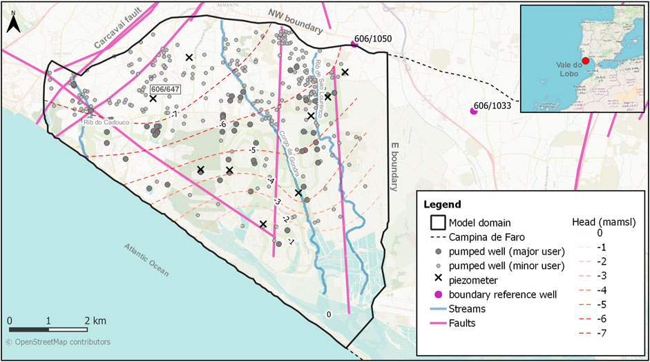
FIGURE 1. Location and main hydrogeological features of the Vale do Lobo aquifer system. The locations of groundwater abstraction wells, piezometers, and contoured average measured hydraulic heads during 2020 are also depicted.

2.1 Conceptual Model

The Vale do Lobo (VL) subsystem of the Campina de Faro aquifer occupies an area of about 32 km². The boundary which separates it from the Campina de Faro subsystem to its east is a management rather than a hydrogeological boundary; it runs roughly perpendicular to topographic contours. To the northwest, the VL subsystem boundary is defined by the Carcavai fault zone. Low permeability marls outcrop along the northern boundary; this creates a barrier between the VL system and a highly permeable karstic aquifer further to the north.

The VL subsystem is comprised of two aquifers. An upper, phreatic aquifer and a lower, semi-confined aquifer formed of calcareous sandstones and limestones. Nearby and offshore drilling suggests that the base of the semi-confined aquifer reaches a depth of 350 m below mean sea level at the coast. A clay aquitard, typically about 10 m thick, separates the two aquifer formations. The aquifer formations dip towards the coast at about 4°. Fresh water that flows seaward through the deep aquifer emerges in the sea at an unknown distance offshore. However, the offshore perseverance of the overlying aquitard, together with all other details of offshore freshwater flow and the geology which controls it, are unknown.

Figure 2 displays heads measured in a representative well (see the labelled location in Figure 1). The well is open to the deep aquifer. This is the longest record of piezometric heads available in the VL area. It exhibits a gradual decline from the late 1970s to the late 1990s, at which time groundwater levels appear to reach a new equilibrium. Groundwater heads are, on average, below sea level in the deep aquifer. The lowest levels are in the central and north-western corner of the system. Groundwater appears to flow towards this area of depressed heads from all system boundaries, including from adjacent aquifers and from the coast.

FIGURE 2

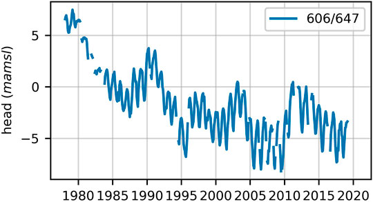
FIGURE 2. Time-series of hydraulic heads measured in piezometer 606/647. The location of this piezometer is labelled in Figure 1.

The local regulatory agency estimates that total groundwater use during 2019 was around 6.45 Mm³. Most of this water was extracted from the deep aquifer. Diffuse recharge to the phreatic aquifer is estimated to be about 3.46 Mm³/yr (i.e., 108 mm/yr). The proportion of this water which reaches the deep aquifer is unknown. The deep aquifer probably receives most of its recharge laterally through its northern and/or eastern boundaries.

Chloride concentrations measured at observation wells within the deep aquifer are mostly below 300 mg/L. However, these measurements, as well as anecdotal evidence pertaining to the quality of water extracted from production wells, suggest increasing salinities over time at some locations. There is some evidence that dissolution of evaporites that are disseminated through sediments which comprise the deep aquifer may be partly responsible for increased chloride concentrations. It appears, therefore, that VL groundwaters have not yet suffered a serious decline in quality because of seawater intrusion. Nevertheless, hydraulic head data makes it clear that its occurrence is inevitable.

2.2 The Problem

Continued extraction of water from the VL system at current rates is unsustainable. In the long term, it will result in serious degradation of aquifer water quality through seawater intrusion. In the short term, it will occasion noncompliance with an EU Water Framework Directive (WFD) which specifies that average abstraction from a groundwater system must be lower than 90% of average annual recharge. Local authorities are looking at a number of ways to comply with this directive. These include the impositions of limits on existing water use licenses and/or implementation of managed aquifer recharge (MAR). However, technical and legal obstacles presently impede both of these options.

Modelling that is described herein serves to:

1) Estimate the historical components of the VL water budget, along with their uncertainties. These include calculation of groundwater withdrawals where records are unavailable, and quantification of lateral inflows from neighbouring systems. Outcomes of these analyses provide an estimate of the minimum change in water budget required to comply with WFD requirements.

2) Explore management strategies that maximize groundwater use while mitigating the potential for seawater intrusion. Outcomes of these analyses are intended to identify maximum allocation limits for existing groundwater users.

2.3 The Numerical Model

2.3.1 Model Structure

A numerical model was developed in order to explore management options for the VL subsystem. The model is a composite of a constant-density MODFLOW 6 (Langevin et al., 2021) model and eight LUMPREM (Doherty, 2020) models. LUMPREM stands for “lumped parameter recharge model”; LUMPREM models are used to compute irrigation demand, and hence groundwater withdrawal rates employed by the MODFLOW 6 model.

History-matching is undertaken over the period October 2000–October 2020. Unfortunately, records of historical abstraction over this period are incomplete. However, they comprise the only direct measurement of any aspect of the VL subsystem water balance. Other aspects of the water balance must be inferred from the system’s response to this extraction. A single LUMPREM model is used to calculate irrigation demand for each groundwater user group. LUMPREM models are calibrated against measured extraction rates where these are available.

The groundwater flow model employs a single layer. This represents the deeper semi-confined aquifer. Its landward boundaries coincide with that of the VL system described above. To its southwest, the coastline bounds the model domain. Aquifer top and bottom elevations are interpolated from onshore and offshore borehole logs and topographic elevations of outcrops.

The bottom boundary of the VL groundwater model is a no-flow boundary. A general-head boundary (GHB) is ascribed to its top. This simulates the connection of the lower aquifer with the overlying phreatic aquifer. Temporal and spatial variation in GHB heads at each cell are calculated by applying a linear function of surface elevation to measured time series of heads in the phreatic aquifer. Constants of this function are adjustable during history-matching.

All lateral boundaries of the VL model are also simulated using GHBs. For the north-western and eastern boundaries of the VL model, GHB heads vary with time while conductance is time-invariant. Time-varying heads are obtained from time-series of measured heads at representative piezometers; these are spatially interpolated along the boundaries.

2.3.2 Model Parameters

An array of 565 pilot points, distributed throughout the model domain, is employed to represent spatial variation of each of hydraulic conductivity, specific storage and conductance of the aquitard which separates the deep aquifer from the upper aquifer.

Pilot points are also placed along all model boundaries. These are used to represent spatial variation of conductance along these boundaries. They are also used to parameterise spatial variation of heads along these boundaries. However, as stated above, time-varying heads at certain locations along the north-western and eastern model boundaries are informed from heads measured in nearby wells. Hugman et al. (2021) for details.

As stated above, the coastal boundary of the VL model is represented by a continuous, coast-coincident GHB. Heads and conductances along this boundary are parameterised using pilot points. Statistical characterisation of these heads and conductances is discussed next.

Statistical characterisation of model parameters is required for two reasons. It is used in formulation of a regularisation scheme which seeks parameter uniqueness through model calibration. It is also used in calculation of an ensemble of parameter realisations which comprise samples of a parameter probability distribution. Prior means and probability density functions for hydraulic conductivity, specific storage and aquitard conductance can be assigned on the basis of expert knowledge. Expert knowledge can also be employed in assigning prior means and standard deviations to pilot points which represent heads along the north-western and eastern boundaries. Conductances along these boundaries are not well informed by expert knowledge; hence large prior uncertainties must be assumed. Fortunately, they are moderately well constrained through history matching.

The assignment of prior means and variances/covariances to coastal GHB boundary heads and conductances is a different matter. These parameters are somewhat abstract, as they are numerical surrogates for complex off-shore processes whose details are poorly known. However, there are physical and geometric constraints on these offshore processes that are set by local geology and the mechanics of density-dependent groundwater flow. Conceptually, these can be used to place constraints on the values of coastal GHB boundary parameters. It is to this subject that we now turn.

3 The Coastal Boundary Condition

3.1 General

Confined and semi-confined coastal aquifers can convey fresh groundwater 10 s or even 100 s of kilometres beyond the coast (Post et al., 2013; Knight et al., 2018). In confined systems, fresh groundwater discharges where the permeable formation outcrops on the seabed. In semi-confined systems, freshwater percolates through the overlying low permeability formation, reaching the sea as diffuse discharge along its bed. The offshore extent of freshwater in the latter case is determined by the hydraulic characteristics of the system and the stresses to which it has been subjected.

Data on offshore and under-sea conditions is rarely available. Stresses that determine the nature of present-day freshwater outflow can date back thousands of years. Explicit (necessarily stochastic) representation of these conditions in the same model as that which is used for aquifer management may require extension of the model grid tens of kilometres offshore; it may also require a long “wind-up” time in which the system is subjected to uncertain stresses. In conducting this modelling, the effects of density differences cannot be ignored.

For exploration of VL aquifer management options, we represent offshore conditions implicitly using a GHB. Meanwhile, constant density, freshwater conditions are assumed to prevail under land. This is in accordance with current assessments of the VL subsystem. A single-layer, fast-running model can then be used for assimilation of onshore data and probabilistic exploration of management options.

3.2 Conditions at the Boundary

Water enters or leaves a GHB in proportion to the difference between the head assigned to the boundary and that calculated by the model for the cell which the boundary occupies. The constant of proportionality is the boundary’s conductance. For a coastal boundary condition, the head ascribed to the GHB represents a head at some point offshore. GHB conductance represents the resistance to flow between the model cell (i.e., the coast) and that point. Conceptually, the coastal GHB can provide simplified numerical representation of the hydraulic linkage between the model and an offshore portion of the same system. However, this simplification ignores the effects of changes in offshore storage while assuming that the dynamics of offshore flow do not change drastically throughout the simulated period.

Use of a GHB to represent a coastal system which is at equilibrium resembles an approach recommended by Lu et al. (2015). However real-world, coastal aquifer systems are rarely at equilibrium. Semi-confined coastal aquifers in particular can take a very long time to reach a new equilibrium because of the relatively slow movement of the fresh-saltwater interface, and the potentially large volume of water stored offshore (Knight et al., 2018). Matters are further complicated when the purpose of modelling is to assess the long-term consequences to a system of a change in onshore pressures.

A GHB that attempts to alleviate the need to simulate offshore conditions must be capable of representing the range of conditions to which the onshore part of the aquifer is subjected. In the current case these conditions are 1) those which prevailed prior to development, 2) those which prevailed in the last few decades when water extraction induced a landward hydraulic gradient, and 3) those which will prevail in the future when groundwater withdrawals are reduced in order to promote aquifer sustainability.

Figure 3 illustrates the first two of these conditions. Conditions in the future lie between these two extremes. The methodology that we now describe provides a statistical characterisation of GHB parameters that can emulate these conditions. Its use is based on the premise that offshore processes can be represented by time-invariant boundary conditions over the simulation time of the VL model. We demonstrate below that this is actually the case.

FIGURE 3

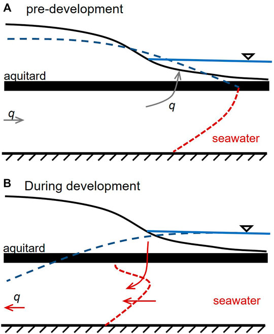
FIGURE 3. Schematic representation of (A) emergence of fresh water through the aquitard overlying a semi-confined aquifer under pre-development conditions, and (B) landward flow of water under conditions that result in active seawater intrusion (adapted from Hugman et al., 2021).

3.3 Stochasticity of GHB Parameters

Before describing the methodology through which a prior probability distribution can be ascribed to GHB parameters, we describe the manner in which the stochasticity of these parameters is represented. We then describe how values of variables which define this representation can be derived through strategic use of a density-dependent model to represent the range of possible offshore conditions.

Let the vector h represent heads ascribed to pilot points that are used to parameterize the coastal model boundary of the VL management model; let the vector c represent pilot point conductances. Collectively, boundary parameters are therefore represented by the composite vector $\left[\begin{array}{c}\mathbf{h}\\ \mathbf{c}\end{array}\right]$. Stochastic representation of boundary parameters requires that mean values be provided for these parameters at the locations of all pilot points; these mean values are represented by the vector $\left[\begin{array}{c}\underset{¯}{h}\\ \underset{¯}{c}\end{array}\right]$. It also requires that a covariance matrix $C\left(\left[\begin{array}{c}\mathbf{h}\\ \mathbf{c}\end{array}\right]\right)$ be ascribed to these parameters. This covariance matrix is used to represent spatial correlation between parameters of the same type at each pilot point along the boundary, as well as correlation between parameters of different types. We assume a Gaussian probability distribution; note, however, that this assumption is not invoked until realisations of boundary parameters are generated for use during stochastic history-matching. Meanwhile prior means, together with the prior covariance matrix, form the basis of regularized inversion through which model calibration is achieved.

Characterization of Stochasticity using a Density-Dependent Model.

The prior mean vector and the prior mean covariance matrix of the $\left[\begin{array}{c}\mathbf{h}\\ \mathbf{c}\end{array}\right]$ parameter set which characterize the coastal boundary of the VL model are obtained through a two-step process. The first of these steps samples a one-dimensional counterpart of $\left[\begin{array}{c}\mathbf{h}\\ \mathbf{c}\end{array}\right]$. We refer to this vector as $\left[\begin{array}{c}h\\ c\end{array}\right]$; it possesses just two elements (each of them random), namely a single head h and a single conductance c. Once enough samples of $\left[\begin{array}{c}h\\ c\end{array}\right]$ have been obtained, its mean $\left[\begin{array}{c}\underset{¯}{h}\\ \underset{¯}{c}\end{array}\right]$ and covariance matrix $C\left(\left[\begin{array}{c}h\\ c\end{array}\right]\right)$ can be estimated. Samples of $\left[\begin{array}{c}h\\ c\end{array}\right]$ are obtained by running a two-dimensional, cross-section, variable density model many times, using random samples of hydraulic properties and geometry which are representative of the offshore VL aquifer system.

In the second step, the stochastic description of $\left[\begin{array}{c}h\\ c\end{array}\right]$ is modified to provide a stochastic description of $\left[\begin{array}{c}\mathbf{h}\\ \mathbf{c}\end{array}\right]$. That is, a mean $\left[\begin{array}{c}\underset{¯}{h}\\ \underset{¯}{c}\end{array}\right]$ vector and a covariance matrix $C\left(\left[\begin{array}{c}\mathbf{h}\\ \mathbf{c}\end{array}\right]\right)$ are determined. Once these are available, random realizations of $\left[\begin{array}{c}\mathbf{h}\\ \mathbf{c}\end{array}\right]$ can be generated through standard statistical sampling. Details of the manner in which C $\left(\left[\begin{array}{c}\mathbf{h}\\ \mathbf{c}\end{array}\right]\right)$ is obtained are provided in Supplementary Material. Briefly, the steps are as follows:

1) Assume a correlation length for h and c along the boundary. This is a heuristic decision that supports representation of spatial variability of these variables along the boundary, while suppressing its expression on too short or too long a spatial scale.

2) Determine the variance of h and c and the correlation between h and c from strategic deployment of a suite of random, one-dimensional, sectional models in the manner described below.

3) Use linear algebra (see Supplementary Material) to derive expressions for $\left[\begin{array}{c}\underset{¯}{h}\\ \underset{¯}{c}\end{array}\right]$ and C $\left(\left[\begin{array}{c}\mathbf{h}\\ \mathbf{c}\end{array}\right]\right)$ based on the above information

Details are provided in Supplementary Material.

3.4 Details of the Density-dependent Model

A stochastic, physically based model of the offshore system is used to obtain samples of $\left[\begin{array}{c}h\\ c\end{array}\right]$. The model is coarse, but reflects the properties, geometry and dynamics of the real-world VL system.

Figure 4 depicts the domain of a two-dimensional, cross-sectional, density dependent SEAWAT model (Langevin et al 2008). This model simulates conditions which are illustrated schematically in Figure 3. Part of its domain lies beneath land, and part of its domain lies beneath the sea. The model simulates head-driven flow of water through a confined aquifer and under-sea emergence of water through a semi-confining aquitard.

FIGURE 4

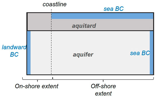
FIGURE 4. Schematic representation of a two-dimensional, density-dependent, cross-sectional model (adapted from Hugman et al., 2021).

An ensemble of model realizations is constructed. Each realization of the model is endowed with random hydraulic properties, a random landward boundary head, and randomized aspects of its geometry sampled from uniform or log-uniform distributions representative of those that characterize the VL subsystem. Table 1 lists aspects of model design which vary between realizations.

TABLE 1

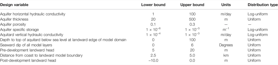
TABLE 1. Aspects of the design of the density-dependent model which vary between realizations.

For each model realization, aquifer and aquitard properties are homogeneous within their respective subdomains. However, they are different between realizations. On the seaward side of the coast, a constant-head boundary is introduced to all top-layer cells and along the vertical model boundary; the head is equivalent to 0 m of salt water. Cells comprising the vertical landward model boundary are assigned a uniform freshwater head. Depending on the model stress period, this is either positive (i.e., above sea level) to simulate pre-development conditions, or negative (i.e., below sea level) to simulate present-day, extractive conditions. The value of landward heads is randomly selected from realization to realization. The distance from the coast to the landward model boundary also varies from realization to realization. Collectively, the range of post-development landward heads, and onshore distances to these heads, encompass those which presently prevail in the VL subsystem.

For each realization, the model is first run under pre-development conditions until equilibrium is established. It is then run for a 50-year period in which landward head is set in accordance with present-day conditions. Fifty years corresponds to the time over which groundwater has been extracted from the VL subsystem. The last 20 years of the last period are thus representative of conditions which prevailed during history-matching of the VL management model described above. For each realization, time series of simulated concentrations and heads at the coastline, together with budget components, are recorded.

Over all realizations the location of the toe of the interface varies from 30 km offshore to 500 m onshore. Figure 5 shows the freshwater head at the coast plotted against time for the 100 realizations that were employed for this study. For most realizations, a sudden change in head occurs shortly after landward extraction of water commences. The head remains reasonably constant thereafter.

FIGURE 5

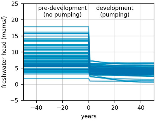
FIGURE 5. Simulated freshwater heads at the coast during pre-development and development conditions simulated by the cross-section model.

The difference in head across the coastline between pre-development and development conditions is used to determine values of h and c for a single realization of the VL model GHB. For any one realization of the density-dependent model, let the freshwater head at the coastline be H_o when water flows toward the sea (i.e., under pre-development conditions), and H_i when water flows toward the land (i.e. under post-development conditions). Values of H_o and H_i are easily obtained from outputs of this model; a value for H_i is established by averaging model-calculated coastal heads over the development period.

Let q_o and q_i denote flow of water (fresh and saline) under the coastline during pre- and post-development conditions. Note also that q_i and q_o have opposite signs. We wish to describe flow across the coastal boundary using a GHB with head h and conductance c. Under outflow conditions:

${\mathit{q}}_{\mathit{o}}=\mathit{ }\left({\mathit{H}}_{\mathit{o}}-\mathit{h }\right)\mathit{c}(1)$

while under inflow conditions:

${\mathit{q}}_{\mathit{i}}=\mathit{ }\left({\mathit{H}}_{\mathit{i}}-\mathit{h }\right)\mathit{c}(2)$

These two equations can be solved for the two unknowns h and c. The solutions are:

$\mathit{c}=\mathit{ }\frac{{\mathit{q}}_{\mathit{o}}-\mathit{ }{\mathit{q}}_{\mathit{i}}}{{\mathit{H}}_{\mathit{o}}-\mathit{ }{\mathit{H}}_{\mathit{i}}\mathit{ }}(3)$

$\mathit{h}=\mathit{ }\frac{{\mathit{q}}_{\mathit{o}}{\mathit{H}}_{\mathit{i}}\mathit{ }-\mathit{ }{\mathit{q}}_{\mathit{i}}{\mathit{H}}_{\mathit{o}}}{{\mathit{q}}_{\mathit{o}}-\mathit{ }{\mathit{q}}_{\mathit{i}}}(4)$

By running the two-dimensional, sectional, density-dependent model many times, many different values of $\left[\begin{array}{c}h\\ c\end{array}\right]$ can be obtained using Equations (3), (4). Values of $\left[\begin{array}{c}\underset{¯}{h}\\ \underset{¯}{c}\end{array}\right]$ and C $\left(\left[\begin{array}{c}\mathbf{h}\\ \mathbf{c}\end{array}\right]\right)$ can then calculated in the manner described above and in Supplementary Material.

4 History-Matching and Deployment of the VL Management Model

Only a brief description of history-matching and deployment of the VL model is provided here. For more details, see Hugman et al. (2021).

4.1 History Matching

History-matching of the VL model was a two-step process. First, parameters were calibrated to obtain a parameter field of minimum error variance using PEST_HP (Doherty, 2021). During this process, parameter uniqueness was attained using preferred-value Tikhonov regularization supplemented with prior parameter covariance matrices to promote parameter field smoothness. An ensemble of 200 parameter realizations was then sampled from a linear approximation to the posterior parameter probability distribution. These were adjusted in order for model outputs to match field measurements using the PESTPP-IES ensemble smoother (White, 2018).

The inversion process featured a total of 2,241 adjustable parameters. These include 211 parameters for the set of LUMPREM models and three sets of 565 pilot point parameters representing hydraulic conductivity, specific storage and aquitard conductance within the VL model domain. The remaining parameters pertain to lateral GHB’s. Of these 58 were used to characterize head and conductance along the coastal GHB.

The history-matching observation dataset included both hard and soft data. LUMPREM-calculated water demands were compared to measured extraction rates recorded by groundwater users where these are available. Simulated heads were compared to borehole heads measured in the piezometric monitoring network. Temporal head differences were also compared; this encourages the history-matching process to replicate seasonal head variations. The calibration dataset also included constraints of minimum heads in abstraction wells and upper limits on lateral recharge.

4.2 Model Deployment

4.2.1 Components of the Water Budget

Compliance with the European Water Directive (WFD) requires evaluation of components of the VL subsystem water balance. Time series of water budget components were computed using 200 samples of the posterior parameter probability distribution calculated by PESTPP-IES. These include flows through the coastal model boundary, through each of the landward model boundaries, and from the overlying unconfined aquifer. It also includes LUMPREM-calculated extraction rates. Figure 6. Time-averaged components of the water balance, together with respective uncertainty standard deviations, are listed in Table 2.

FIGURE 6

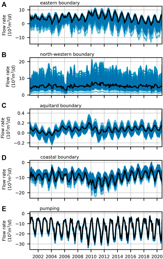
FIGURE 6. Time-series for each of the VL water balance components simulated with the post-history-matching parameter ensemble (blue lines); net flow through the (A) eastern, (B) north-western (C) aquitard and (D) coastal boundaries, and (E) extracted through pumping. The black line highlights time series calculated using the parameter set achieved through model calibration (adapted from Hugman et al., 2021).

TABLE 2

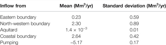
TABLE 2. Water balance of VL aquifer over the history-matching period.

Features of interest in Table 2 include the following:

• Inflow to the deep (exploited) aquifer from the overlying unconfined aquifer comprises only a small component of the overall water balance.

• There is a considerable influx of water to the system from the seaward side of the coastal boundary.

• Inflow to the system from the north-western boundary is large.

• Uncertainties associated with all lateral boundary inflows are large.

The WFD requires that groundwater extraction be less than 90% of average annual (freshwater) recharge in managed groundwater systems such as Vale do Lobo by 2027. This criterion is simplistic and difficult to apply to the VL subsystem, as extraction from the system induces recharge. Nevertheless, if Table 2 is viewed as a static ledger, it can be established that 2.9 ± 1.07 Mm³/yr of extra recharge is required if all non-coastal inflow is to exceed pumping. This value represents the lower limit of additional recharge (or reduced abstraction) that is required to meet WFD requirements. However, it probably underestimates alterations to the current water balance that are required to preclude the threat of saltwater intrusion.

4.3 Optimal Distribution of Extraction

VL irrigation is almost entirely dependent on groundwater extraction. Reduction of extraction is a prerequisite for reducing the risk of seawater intrusion. However, a strategic distribution of extraction locations may mitigate the amount by which extraction must be reduced in order to ensure sustainability.

The VL management model was used to calculate how much water can be extracted from the VL subsystem under the constraint that extraction remains sustainable. Decision variables in this optimisation problem are extraction rates employed by the nine major VL groundwater user groups; it is assumed that the wells from which these groups extract water is unchanged from that which they presently employ. As extraction rates attributed to these user groups change, so too does the geographical distribution of groundwater extraction from the VL subsystem.

Maximization of extraction is subject to a single constraint. This is that there be zero net flow of water landward from the VL coastal boundary into the model domain. We recognise that this constraint does not preclude seawater intrusion. It only ensures net freshwater discharge to the sea. Extraction rates which satisfy this constraint may exceed those that preclude seawater intrusion. Thus, outcomes of this optimisation problem provide an upper estimate of the sustainable rate of extraction from the VL subsystem. More detailed constraints can be imposed if this value is large enough to warrant further investigation. Results presented below suggest that it is not likely to be worth the effort.

4.3.1 Difficulties

History-matching ascribes high conductances to the eastern GHB of the VL model. This indicates that the VL system cannot be managed in isolation. Pumping of the deep aquifer to the east of this boundary lowers groundwater levels within the VL subsystem. (Recall the artificial nature of the VL management boundary.)

To accommodate this issue the optimization problem is solved with five different head distributions ascribed to the eastern GHB, these simulating five different intensities of water extraction from the neighbouring subsystem. The highest of these five head distributions mimic pre-development conditions in which extraction from the neighbouring, easterly subsystem is minimal. The lowest of these five head distributions are slightly above those that characterise present-day conditions. The optimization problem is solved five times, once for each of these boundary head distributions.

To accommodate parameter uncertainty, these optimization problems are solved in two different ways. First the VL model is endowed with a single parameter set, namely the parameter set emerging from model calibration. We refer to these five solutions as “risk neutral”, for they take no account of posterior parameter uncertainty. Ideally the calibrated parameter field, and model predictions that are made using this field, lie somewhere near the centre of their respective posterior probability distributions. These optimization problems are solved using the PESTPP-OPT optimizer that is supplied with the PEST++ suite.

We then solve the optimization problem using the ensemble of parameter sets that were calculated by the PESTPP-IES ensemble smoother. In this case, definition of the optimization constraint is varied to accommodate parameter uncertainty. Groundwater extraction is now optimized under the constraint that inland flow from the coastal boundary is zero or less (i.e., flow is outward) for all 200 parameter fields that comprise samples of the posterior parameter distribution. This simulates the operation of a risk-averse management strategy. This optimization-under-uncertainty problem is solved using the CMAES_HP global optimizer (supplied with PEST_HP).

4.3.2 Results

Risk neutral and risk averse solutions to the optimization problem are depicted in Figures 7A–C. The vertical axis of Figure 7A expresses optimal total extraction as a fraction of current extraction; the horizontal axis expresses conditions at the eastern boundary using an observation well that is close to this boundary. Figure 7B, C depict the distribution of optimized extraction between user groups. The major groundwater users in the area are several golf courses, an area of intensive agriculture and distributed small users. They are intentionally not named in Figure 7 for privacy.

FIGURE 7

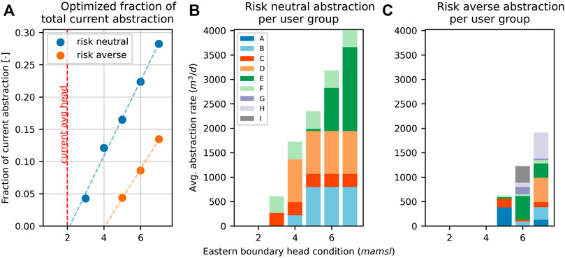
FIGURE 7. (A) Solutions to constrained extraction optimization problems and, relative extraction rates for different user groups for (B) the five solutions of the risk neutral optimization problem and (C) the three solutions of the risk averse optimization problem (adapted from Hugman et al., 2021).

As stated above, the lowest of the five head distributions attributed to the eastern GHB corresponds to heads that are slightly above those that are currently being experienced. Figure 7A demonstrates that it is not possible to obtain a feasible solution to the constrained optimization problem under head conditions that are any lower than this, including those which characterise present-day conditions. It follows that if water use on the other side of the eastern boundary continues at its current rate, any extraction from the VL aquifer is unsustainable regardless of the risk stance. This is because eastern groundwater extraction induces landward flow of water through the VL subsystem. The VL subsystem cannot be managed in isolation.

5 Discussion and Conclusion

5.1 The “Simple” Model Setup

It is apparent from the above description that construction, calibration and deployment of the simple model that is described herein requires a rather complicated workflow. The model is “simple” in that it runs fast and is numerically stable; this is achieved by representing processes and structure through simple functions and boundary conditions. All of these are customized, this requiring that software be written for their implementation and parameterisation. Fine-tunning this setup required some trial-and-error; the workflow was revised many times as modelling proceeded. This is not an uncommon occurrence in real-world, decision-support modelling. The advent of new information, and lessons that are painfully learned during model development, frequently require that modelling plans be considerably revised. Fortunately, all components of all of the workflows that are outlined in this paper are scripted. Furthermore, the run time of the management model is small. This allowed rapid experimentation and testing of different ideas in ways that were flexible and reproducible.

All real-world modelling is difficult. Innovation is a necessity. “Back to the drawing board” moments are common. The advantages of reproducibility and reduced mental overhead that are enabled by a scripted workflow and a structurally simple model cannot be overemphasized.

5.2 Complementary Models

This paper demonstrates how abstract, non-physical parameters that characterise the boundary conditions of a fast-running, decision-support model can be informed by expert knowledge. This enables derivation of the prior expected values of boundary condition parameters, as well as characterisation of the prior uncertainties of these parameters. This obviates the need for non-informative priors whose use may unnecessarily inflate the posterior uncertainties of decision-critical model predictions.

The methodology described herein is based on the conjunctive use of two models. One of these models is complex. Its role is to simulate system structures and processes that are represented in an abstract manner in a complementary, simple, fast-running model that is designed with data assimilation and uncertainty quantification in mind. Simulation of hydrogeological complexities by the complex model cannot be exact, for many of the structures and processes that it includes are only vaguely known. Its task is to represent the ramifications of this vague knowledge for parameters that are assigned to part of the simpler management model—one of its boundary conditions in this case. Representation of this boundary must be stochastic. To the extent that expert-knowledge-informed stochasticity of the complex model can limit the stochasticity of management model boundary parameters, the latter’s role in supporting environmental decision-making is enhanced, for the uncertainties of some of its predictions may thereby be reduced.

It is evident from the above that such an approach is of value in cases where 1) prediction uncertainty is affected by abstract parameter uncertainty and 2) this uncertainty is not reduced through history matching. In such cases, as discussed, expert knowledge can be an important (or only) source of information to constrain decision-pertinent uncertainties.

Figure 8 displays a generalisation of our workflow. It can be summarized as follows:

• A simple model is constructed in which numerically problematic processes and structures are replaced with approximate representations that are populated by non-physically based parameters. Forecasts of interest simulated by the simple model are affected by the uncertainties of these parameters where these cannot be adequately constrained by field observations of system states and fluxes.

• A complementary complex model is constructed which explicitly represents some of the processes and structures that prevail at a study site. Prior probability distributions for parameters of the complex model are characterized using expert knowledge derived from site characterisation. The complex model is populated using an ensemble of parameter fields sampled from this expert-knowledge-informed prior probability distribution. From the outcomes of many complex model runs, equivalent values for the more abstract parameters of the simple model are calculated.

• Samples of abstract parameters which are thus obtained are used to characterize the prior probability distribution of simple model parameters.

• The simple model is then subjected to stochastic history-matching. Posterior parameter probabilities obtained through this process therefore reflect information gained from both measured data and expert knowledge. These are used to explore predictive outcomes of management interest.

FIGURE 8

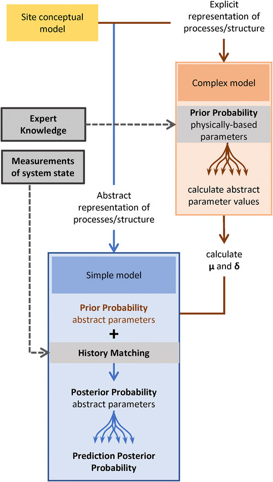
FIGURE 8. Diagram of a workflow that uses complementary models to extract information from both expert knowledge and measurements of system state.

It is safe to say that few, if any, modelling alternatives to the approach that we have documented herein would have enabled data assimilation, uncertainty quantification, and exploration of optimized management strategies for the VL subsystem in ways that were achieved with the present modelling strategy. The option of building a single, complex, density dependent model (an option that is often taken in coastal contexts) would have made high-end data assimilation and uncertainty quantification almost impossible because of long run times and likely numerical instability. These problems would have been exacerbated if the domain of this model was made to extend for a considerable distance under the sea in order to simulate freshwater outflow. This could not have been accommodated in a properly stochastic fashion. Simplifications in representing outflow conditions and testing of only one or a small number of outflow options, may have led to unquantifiable predictive bias.

Decision-support modelling always requires compromises. These compromises do not result in loss of “simulation integrity”, for integrity of simulation is an unachievable goal. If the task of decision-support modelling is properly defined (see, for example Doherty and Moore, 2021), the search for a compromise requires that reduction of uncertainty accrued through assimilation of expert knowledge be traded off against reduction of uncertainty accrued through history-matching. If a model is structurally simple, if may be capable of fitting a history-matching dataset very well. However, if this dataset is not rich in prediction-specific information, the parametric and predictive bias that may be incurred through model structural simplicity, may outweigh the benefits of assimilation of these data. Meanwhile, use of an abstract model design may have precluded parameter value insights gained from expert knowledge of real-world hydraulic properties. The optimal compromise will always be context and prediction specific.

This study demonstrates that selection of an appropriate level of model structural complexity does not always have to be an “either/or” choice. This is because the model that performs data assimilation does not need to be the same model as that which is used to extract information from expert knowledge. Two different models can be used conjunctively for these two different purposes. They can “meet” at a boundary condition of the data assimilation model. The parameters of this boundary condition are thereby provided with prior probability distributions that reflect process and properties that are missing from the model itself, but that may have profound effects on the uncertainties of management-critical predictions.

By separating the tasks of assimilating information that is resident in measurements of system state on the one hand, and assimilating information that is resident in expert knowledge on the other hand, each model can be tuned to its primary task. Fast execution speed and numerical stability are primary requirements for the former task. An ability to represent the range of possible conditions that are compatible with expert knowledge is a primary requirement for the latter task. The “complex” model that was used for the latter task in work that is documented herein, was actually not very complex; it is a two-dimensional sectional model. However, its two-dimensional design enhanced, rather than impeded, its ability to explore a wide range of hydraulic and geometric possibilities for undersea emergence of fresh water off the coast of Vale do Lobo. These possibilities were then made available to the management model through stochastic characterisation of its coastal boundary condition.

5.3 Final Remarks

Decision-support modelling in coastal areas is notoriously difficult. Uncertainties are often high. The potential of available data to reduce these uncertainties may be limited.

This may be a blessing rather than a curse. Compromises must be made. These compromises often require that a modeller identify sources of information that may be most effective in reducing the uncertainties of predictions that he/she cares about. Modelling must then be tuned to extraction of information from these sources without inducing bias or inflating uncertainties by impeding or distorting the flow of information from other sources to too great an extent. However, where uncertainties are already high, the costs in extra uncertainty that are incurred by designing a model, and a modelling workflow, that are optimal for one task but not necessarily another, may not be great in comparison to these inherent, background uncertainties that are born of information insufficiency. This gives a modeller the freedom to test different workflows, and then tailor them to suit his/her needs.

We have demonstrated in this paper that strategic use of complementary models may make modelling choices less painful. A “win/lose” choice can be transformed into a “win/win” choice. We have also attempted to demonstrate that where innovation is required, the use of automated workflows allows a modeller to free him/herself from the yoke of having to adhere to one particular workflow. Different options can be rapidly tested. Once a suitable option is discovered, it can be rapidly improved. The cost of exploration becomes remarkably low. The journey of discovery becomes remarkably rewarding.

Data Availability Statement

Data pertaining to modelling of the real-world case study is proprietary and cannot be shared. Data for the synthetic case can be provided on request. Requests to access the datasets should be directed to rui.hugman@flinders.edu.au.

Author Contributions

RH and JD conceived the idea. RH analysed the data, set up the modelling workflows and undertook all simulations and their postprocessing. JD derived the solution to obtain the stochastic characterization of spatially distributed parameters. JD implemented adaptations to MODFLOW6 and prepared PEST_CMAES setups. Both authors discussed the results and contributed to the final manuscript.

Funding

This work was undertaken through the “Groundwater Modelling Decision Support Initiative” (GMDSI), conducted under the auspice of the National Centre for Groundwater Research and Training (NCGRT), Flinders University, South Australia with funding from BHP and Rio Tinto.

Conflict of Interest

The authors declare that the research was conducted in the absence of any commercial or financial relationships that could be construed as a potential conflict of interest.

Publisher’s Note

All claims expressed in this article are solely those of the authors and do not necessarily represent those of their affiliated organizations, or those of the publisher, the editors and the reviewers. Any product that may be evaluated in this article, or claim that may be made by its manufacturer, is not guaranteed or endorsed by the publisher.

Acknowledgments

We thank Kathleen Standen (University of the Algarve) for her contributions to gathering and processing data for the Vale do Lobo case study reported in this paper.

Supplementary Material

The Supplementary Material for this article can be found online at: https://www.frontiersin.org/articles/10.3389/feart.2022.867379/full#supplementary-material

References

Doherty, J., and Moore, C. (2020). Decision Support Modeling: Data Assimilation, Uncertainty Quantification, and Strategic Abstraction. Groundwater 58, 327–337. doi:10.1111/gwat.12969

PubMed Abstract | CrossRef Full Text | Google Scholar

Doherty, J., and Moore, C. (2021). Decision Support Modelling Viewed through the Lens of Model Complexity. A GMDSI Monogr. South Australia: National Centre for Groundwater Research and Training, Flinders University. doi:10.25957/p25g-0f58

CrossRef Full Text | Google Scholar

Doherty, J., and Simmons, C. T. (2013). Groundwater Modelling in Decision Support: Reflections on a Unified Conceptual Framework. Hydrogeol. J. 21, 1531–1537. doi:10.1007/s10040-013-1027-7

CrossRef Full Text | Google Scholar

Doherty, J. (2021a). PEST_HP PEST for Highly Parallelized Computing Environments. Brisbane: Watermark Numerical Computing.

Google Scholar

Doherty, J. (2021b). Version 2 of the LUMPREM Groundwater Recharge Model. Brisbane: Watermark Numerical Computing.

Google Scholar

Freeze, R. A., Massmann, J., Smith, L., Sperling, T., and James, B. (1990). Hydrogeological Decision Analysis: 1, A Framework. Groundwater. 28, 738–766.

CrossRef Full Text | Google Scholar

Hugman, R., Doherty, J., and Standen, K. (2021). Model-Based Assessment of Coastal Aquifer Management Options. A GMDSI Worked Example Report. South Australia: National Centre for Groundwater Research and Training, Flinders University. doi:10.25957/a476-x588

CrossRef Full Text | Google Scholar

Knight, A. C., Werner, A. D., and Morgan, L. K. (2018). The Onshore Influence of Offshore Fresh Groundwater. J. Hydrol. 561, 724–736. doi:10.1016/j.jhydrol.2018.03.028

CrossRef Full Text | Google Scholar

Langevin, C. D., Thorne, D. T., Dausman, A. M., Sukop, M. C., and Guo, Weixing. (2008). SEAWAT Version 4: A Computer Program for Simulation of Multi-Species Solute and Heat Transport: U.S. Geological Survey Techniques and Methods Book 6, 39 p. U.S. Geological Survey, Reston, Virginia.

Google Scholar

Langevin, C. D., J. D, Hughes, E. R, Banta, A. M, Provost, R. G, Niswonger, and S, Panday. (2021). MODFLOW 6 Modular Hydrologic Model Version 6.2.2: U.S. Geological Survey 652 Software Release, 30 July 2021. doi:10.5066/F76Q1VQV

CrossRef Full Text

Lu, C., Werner, A. D., Simmons, C. T., and Luo, J. (2015). A Correction on Coastal Heads for Groundwater Flow Models. Groundwater 53, 164–170. doi:10.1111/gwat.12172

CrossRef Full Text | Google Scholar

Post, V. E. A., Groen, J., Kooi, H., Person, M., Ge, S., and Edmunds, W. M. (2013). Offshore Fresh Groundwater Reserves as a Global Phenomenon. Nature 504, 71–78. doi:10.1038/nature12858

PubMed Abstract | CrossRef Full Text | Google Scholar

White, J. T., Doherty, J. E., and Hughes, J. D. (2014). Quantifying the Predictive Consequences of Model Error with Linear Subspace Analysis. Water Resour. Res. 50, 1152–1173. doi:10.1002/2013WR014767

CrossRef Full Text | Google Scholar

White, J. T. (2018). A Model-independent Iterative Ensemble Smoother for Efficient History-Matching and Uncertainty Quantification in Very High Dimensions. Environ. Model. Softw. 109, 191–201. doi:10.1016/j.envsoft.2018.06.009

CrossRef Full Text | Google Scholar